Regional climate trend analyses for Aqua MODIS land surface temperatures

ABSTRACT

Land surface temperature (LST) is the skin surface temperature of the Earth’s land surface and is an essential climate variable (ECV) that critically characterizes the Earth’s climate and surface energy processes. This is the first regional trend analysis for LST with uncertainties, using a stable LST climate data record suitable for climate trend analyses: the Aqua Moderate Imaging Spectroradiometer (MODIS) dataset (MYDCCI) produced in the European Space Agency (ESA) LST Climate Change Initiative (LST_cci) Project. The quality of the trends is verified here for Western Europe, for which consistent trends per decade of 0.5 K and 0.57 K across daytime and night-time data, respectively. Eight regions representative of a range of biomes and, including the Amazon, Western U.S.A., Greenland, the Sahel, Siberia, China, India, and Australia, have been analysed. Our most significant findings show substantial LST increases for Siberia and the Amazon, as well as evidence of recent increasing trends for the Western U.S.A. Siberia showed the most substantial daytime and night-time changes per decade of +0.87 K and +0.93 K, respectively. Furthermore, the Amazon and Western U.S.A. showed significant daytime LST trend increases of +0.82 K and +0.51 K, respectively. Western Europe and Western U.S.A. show the largest night-time change of +0.57 K and +0.54 K, respectively. India presents an atypical time series with a decreasing daytime and increasing night-time trend per decade of −0.62 K and +0.44 K, respectively, consistent with reported air temperatures. Overall the results show significant positive regional LST trends, against a background of both strong seasonal cycles and intermittent disruptive events, which demonstrate the importance of continued LST observations. The results also incentivize remote sensing science to derive ever more rigorous LST datasets and to continue to investigate emissivity and error correlations to allow improved trend analyses for smaller regions and individual locations.

KEYWORDS:

• Land surface temperatures
• Earth Observation Science
• time series analysis
• climate trends
• aqua MODIS

1. Introduction

Land surface temperature (LST) is defined as the skin temperature of the Earth’s surface, which approximates the thermodynamic temperature as a measurement of radiance on regional and global scales (Norman and Becker 1995). LST is a key measurement of surface energy processes (Duan, Li, and Leng 2017) that drives outgoing radiation and heat fluxes between the atmosphere and land (Hulley and Ghent 2019). It is described by the Global Climate Observing System (GCOS) as an essential climate variable (ECV) (Belward et al. 2016). ECVs are significant variables that critically characterize Earth’s climate by providing evidence supporting climate science and predicting future change (Popp et al. 2020). LST is usually retrieved via multi – band measurements in the thermal infrared (TIR) wavelength range by remote sensing, which aids in the determination of Earth’s radiative energy budget (Box and Box 2016). The theoretical foundation on which remote sensing is based according to Planck’s law is that the total energy emitted by the surface strictly increases with a rise in temperature. This allows for Earth observations to be retrieved from orbiting space – borne satellite instruments (Hulley and Ghent 2019).

Satellite LST data are used in climate science to analyse surface temperature trends and are a significant factor in understanding the global energy balance (Weng 2009). Surface temperatures help to control the energy partition into latent and sensible heat within the lower atmosphere and are used to determine surface energy and radiation exchange (Liu, Hagan, and Liu 2020). As an indicator of strong surface warming trends, LST is a key, quantifiable physical measurement that determines Earth’s radiative energy flux (Tomlinson et al. 2011). LSTs vary across Earth, and with a lack of in situ data, especially for remote regions, satellite observations are becoming increasingly significant for global and regional climate applications (Li et al. 2023). LST retrievals provide spatially continuous measurements that are crucial for the analysis of global surface temperature changes in response to natural and anthropogenic forcing (Hulley and Ghent 2019). Many climate and weather scientific challenges depend on LST knowledge such as climate modelling inputs, data assimilation, numerical weather prediction, forecasting, and reanalyses, weather event monitoring and crop management, and land – atmosphere climate feedbacks (ESA 2021). Therefore, robust satellite LST observations are crucial for a better understanding of global climate trends.

The significance and versatility of satellite LST data have previously been demonstrated for a variety of applications across Earth. For example, Wan, Wang, and Li (2010) used thermal properties from a normalized difference vegetation index (NDVI) with surface temperature data to monitor droughts in the southern Great Plains, U.S.A. Roth (2012) discussed the role of artificial surfaces on rising city temperatures that contribute to the Urban Heat Island (UHI) phenomenon. LST annual cycles have been mapped for the detection of permafrost boundaries to investigate volcanic permafrost degradation impacts under warming conditions in Chile (Batbaatar et al. 2020). Other applications have investigated the physical dynamics and relationships between LSTs, climate cycles, and extreme weather variability. A comparative analysis (Wyss et al. 2022) discussed how the increase in extreme weather patterns, such as extensive droughts, was responsive to surface temperatures in Namibia. Saint-Lu et al. (2019) found interactions between land – surface warming and atmospheric circulations, on rainfall changes over mid – latitudinal tropical rain forests. Retamales-Muñoz, Durán-Alarcón, and Mattar (2019) showed significant surface warming trends in Antarctica by using atmospheric reanalysis alongside satellite – derived LST. And, Westergaard-Nielsen et al. (2018) demonstrated the spatial and seasonal variability of surface temperatures in Greenland. These studies demonstrate the versatility of satellite LST data that is used in many climate and weather applications. Indeed, they reinforce the need for further satellite LST trend analyses to help better understand the significance of surface temperature variability and its impact on climate studies across Earth.

Various existing time series using other satellite LST datasets have demonstrated the significance of surface temperature trend analysis for different regions and have highlighted the non – uniformity of climate change across Earth. Fu and Weng (2016) provided a time series of LSTs that used thermal characteristics to find a relationship between land use and land cover patterns. A more recent study (Li et al. 2022) tested different methods using simulated LSTs to produce a long – term LST time series. LST trend analyses have also been used to link land use changes to degradation in wetland hydrological and evapotranspiration cycles (Muro et al. 2018). Furthermore, Bento et al. (2020) used LST and NDVI index time series to determine the role of surface temperatures in dryland and desert environmental vegetation health. Vecchio et al. (2018) were able to use time-series data of ice surface temperatures and ice velocities, to explain the behaviour of the Viedma glacier, Argentina. Similarly, studies on the spatial patterns of LST were analysed to find strong links to the biophysical effects of Siberian Boreal forest fires (Liu et al. 2018). Some studies on global surface temperature change have also been conducted. For example, Sobrino, Julien, and García-Monteiro (2020) provided surface temperatures for the whole planet as if they were a single pixel, using these trends to correlate against climate model temperature anomalies. Although these time-series studies highlight the value of LSTs for various regional applications, rigour can only be insured with evidence of climate stability of the datasets and a fully traceable uncertainty budget.

Some studies on quantifying LST uncertainties, for different infrared LST instruments on various space – borne satellites already exist but are rarely applied for global climate analyses. For example, Wan (2002) used early MODIS data to present a study of the associated channel – dependent noise and systematic errors. An analysis of the Spinning Enhanced Visible and Infrared Imager (SEVIRI) uncertainties by Freitas et al. (2010) found the uncertainties to be highly dependent on the input accuracy and retrieval conditions of atmospheric water vapour (WV) content and sensor viewing angles. Previous propagations of LST uncertainty components have provided relatively robust functions for quantifying satellite LST retrievals. Uncertainties have been quantified and modelled for a range of retrieval algorithms, including LST and emissivity from the Advanced space – borne Thermal Emission and Reflection Radiometer (ASTER) and MODIS (Hulley and Hook 2012). More recently, Ghent et al. (2017) provided the first classified pixel – level uncertainties of global LSTs from the thermal infrared products of the Leicester Along – Track Scanning Radiometer (ATSR) and the Sea and Land Surface Temperature Radiometer (SLSTR). Further to presenting a new approach to defining uncertainties for MODIS LST (Ghent et al. 2019), which is applied in this paper. However, there are a lack of studies on time series and trend analyses with full uncertainty propagations using a stable dataset.

Remote TIR retrievals require clear skies to determine accurate LST measurements (Tomlinson et al. 2011). The limitation to clear – sky conditions is due to the inability of TIR to penetrate clouds. However, the benefits of TIR surface temperature retrievals far outweigh the clear – sky bias problem. Previous studies comparing TIR satellite LST and near – surface air temperatures (Good et al. 2017) indicate that clear – sky bias is significant in absolute temperature space but not a significant issue in anomaly space. Moreover, TIR satellite remote sensing is effective for measuring global LST anomalies to provide reliable analyses of LST trends and changes (Tomlinson et al. 2011). Therefore, this paper presents an analysis of LST anomalies for regions across Earth representative of various climates and anthropogenic changes between 2002 and 2021, with for the first time a fully propagated uncertainty budget. Here, we provide an analysis of the LST Climate Change Initiative (LST_cci) product from the Moderate Imaging Spectroradiometer (MODIS) aboard the National Aeronautics and Space Administration’s (NASA) Aqua Satellite. This dataset will be referenced in this study as MYDCCI.

LST is a prominent variable in Earth science and crucial to investigating the regions most affected by climate change. This study, therefore, investigates eight regional climate trends using Western Europe as a test region, to test and demonstrate the value of the MYDCCI dataset. Our study provides a natural continuum from previous studies to demonstrate the significance of TIR retrievals using a robust dataset for regional LST anomaly trend analyses.

2. Materials and methods

2.1. Materials

The Aqua MODIS MYDCCI dataset provides LST data and the associated uncertainties at the full pixel level. It also includes emissivity and quality control flag data that have been used for LST retrieval. Previous work (Good et al. 2022) tested the stability of MYDCCI dataset by comparing it with homogenized station air temperatures over Europe. They found the dataset to be free from non – climatic discontinuities and is stable over time, and therefore fit for trend analysis.

NASA’s Aqua satellite provides sun – synchronous bi – daily full – Earth observations. Aqua’s equatorial afternoon overpass from south to north at approximately 13:30, and night-time overpass at approximately 01:30, is ideal for maximum daily LST retrieval (Good et al. 2017). MODIS observes the Earth in 35 spectral bands in wavelengths between 0.4 and 14.4 µm every one to two days (Barnes, Pagano, and Salomonson 1998). The MYDCCI dataset uses a generalized split – window (GSW) algorithm (Becker and Li 1990; Ghent et al. 2019; Wan and Dozier 1996) to estimate LST from bands 31 and 32 centred on 11 µm and 12 µm, based on a linear function of clear – sky top – of–atmosphere (TOA) brightness temperatures (Becker and Li 1990; ESA 2019; Ghent et al. 2017). Retrieval coefficients are determined for different satellite viewing angles and atmospheric water vapour bands. The CAMEL database is used to estimate the Land surface emissivity (LSE), including emissivities at 10.8 µm and 12.1 µm (Hook 2017). The CAMEL database has emissivities for 10 wavelengths between 3.6 µm and 14.3 µm at a spatial resolution of 0.05${ }^{\circ }$.

The MYDCCI data provide TIR observations from 2002 to the present, at a resolution of 0.01${ }^{\circ }$, allowing for the analysis of LST (Ghent et al. 2019). The data level outlines the amount of processing performed from satellite sensor raw data into the geophysical product, therefore the higher the level the more processing has occurred. The data used in this study (MYDCCI), are in the context of the European Space Agency’s (ESA) LST_cci Level 3 collated (L3C) products. The L3C products are daily (day and night separately) composites of the level 2 single swath data, which are collated and mapped onto a 0.01 ${ }^{\circ }$ space – time latitude – longitude grid. Where multiple swaths cross during the day or night at higher latitudes, the data closest to the nominal local overpass time is used. The combination of multiple sets of observations is stored in single data arrays for a temporal resolution, of which Aqua MYDCCI L3C serves separate day and night files (ESA 2021).

2.2. Methodology

2.2.1. Temperature trends

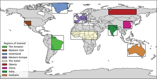
LST anomalies and their associated uncertainty budgets were initially tested for Western Europe, a region where previous studies (Good et al. 2022) have proven the MYDCCI dataset to be stable over time and fit for climate trend analysis. Thereafter, the methods were applied to eight other regions of interest (ROI) including the Amazon, Western U.S.A., Greenland, the Sahel, Siberia, China, India, and Australia described in Figure 1. These regions were chosen as representative areas of different biomes and climates, with a range of surface types and characteristics that might be affected by climatic and anthropogenic changes. As surfaces across Earth are subjected more to human and climatic influence, it is important to monitor and analyse the trends and changes to further understand LST variability.

Figure 1. Regions of interest across Earth used in this study of LST anomalies and their associated uncertainty budget. The ROIs are defined and identifiable by the latitude and longitude used in the MYDCCI data extractions. Going clockwise from left to right, the study regions include the Amazon, Western United States of America (U.S.A.), Greenland, Western Europe, the Sahel, Siberia, China, India, and Australia. An LST anomaly time series and uncertainty budget was produced for each region.

A temperature anomaly describes the difference from a baseline climatology. The anomalies were calculated by fitting a linear trend using ordinary least squares that measure the departure from defined LST means (Stephens et al. 2018). This method is effective in revealing non-seasonal variability and abnormal indices by removing the annual cycle from the data. Positive and negative anomalies are indicative of warming and cooling from the baseline climatology of the full MYDCCI archive (2002–2021), respectively (Spies 2006). The monthly anomalies and their temperature change per decade calculated for the study regions are less affected by the TIR clear – sky bias (Good et al. 2017) and therefore represent a more reliable temperature trend series than the absolute equivalent values.

2.2.2. Applied propagation of uncertainties

A further analysis presents the first applied uncertainty budget (Ghent et al. 2019) for almost two decades between 2002 and 2021 of MYDCCI LSTs. Determined by the Joint Committee for Guides in Metrology, uncertainties quantify what is unknown about the LST value returned and whether it is a correct reflection of the ‘ground truth’ (Joint Committee for Guides in Metrology 2008). Remote sensing data are not the same as ground data and involve unknown errors. An error is the result of a measurement minus the true value (usually known) of the measured quantity, which determines the ‘wrongness’ of a value. For satellite – derived LSTs, the true values cannot be determined. Therefore, uncertainty estimates the doubt around that measurement given our existing knowledge of the data and the effects causing the error (Merchant et al. 2017). Surface temperature observations have an associated uncertainty budget due to the effects of atmospheric attenuation and surface emissivity variability. Uncertainty information provides an estimate of the true gaps in our knowledge of the data retrieved. Its propagation allows us to critically assess the associated climate trend analyses, without which it would provide weak results. Understanding the uncertainties enhances the full comprehension of the surface data reported and allows for the identification of areas for future improvements.

In the case of the MYDCCI dataset, the uncertainty budget is split into components arising from errors that correlate on different spatial and temporal scales (Joint Committee for Guides in Metrology 2008) and (Ghent et al. 2019). For each pixel, these components are random, locally correlated, and large – scale systematic. The uncertainty budget comprises the following five components. Random includes satellite sensor background noise that is uncorrelated on all spatial and temporal scales. Systematic uncertainties of simulated instrument channel radiance from the radiative transfer model and instrument calibration are assumed to be correlated on all spatial and temporal scales. Locally correlated uncertainties include atmospheric and surface components, which are estimated in the standard deviation of the difference between simulated input and retrieved surface temperatures. Atmospheric water vapour may be treated as correlated within its correlation length scale of up to 0.5 km and 5 min (Steinke et al. 2015), whereas surface emissivity is assumed to be correlated, within the correlation length scale of 0.5 km and 1 month (Ghent et al. 2017). The sampling uncertainty component estimates the uncertainty caused by undersampling a grid cell when the cloud is present. A grid cell variance is used to weight the clear – sky bias uncertainty. The sampling uncertainty is propagated at random on all scales (Ghent et al. 2019). Errors due to mis – classification of clouds and geolocation errors are not included in the uncertainty budget and may result in an underestimate of the total uncertainty for some pixels. It is important to be aware that the final scene uncertainty comes with a degree of its own uncertainty, relating to the assumed correlation length scales, which vary on geographical and seasonal scales. The essential conclusion is that water vapour correlations are not as important over a wide area, as they do not propagate in time. Whereas, emissivity correlations affect matter across monthly boundaries and therefore may inject a small amount of autocorrelation. By choosing large regions of interest, the total uncertainty is close to the value of the systematic component. For each individual LST pixel, the total uncertainty can be obtained by summing each of the five uncertainty components in quadrature (Ghent et al. 2019). The uncertainty propagation is used to reflect the robustness, as well as provide critical information about the MYDCCI dataset.

Statistically, the propagation of uncertainties is the variable effect on the uncertainty of the function they are based on. The components are propagated using the methodology of Ghent et al. (2019), as random or correlated, which is determined by understanding what properties a singular pixel shares with other nearby and distant pixels. This method defines the total cell uncertainty estimation (1), which was applied to the MYDCCI L3C data set for various climates across Earth specified as ROIs in Figure 1.

(1) $u_{cell}^2=\frac{1}{\sum N_{\bar{c}}}(\frac{{\sum }_{i=\bar{c}}{u}_{ran}^2}{\sum N_{\bar{c}}})+\frac{{\sum }_{i=\bar{c}}{u}_{loc,atm}^2}{\sum N_{\bar{c}}}+\frac{{\sum }_{i=\bar{c}}{u}_{loc,sfc}^2}{\sum N_{\bar{c}}}+u_{sys}^2+\frac{N_{c}Va{r}_{LST}}{N_{\bar{c}}+N_c-1}$(1)

The grid scene $(u_{cell}^2)$ tries to capture the data sampling based on a number of individual pixels (i), where more clear – sky pixels $(N_{\bar{c}})$ reduce uncertainty and more cloudy sky $(N_c)$ pixels increase uncertainty. The total number of pixels is the sum of those pixels where an LST estimate exists. For clear – sky observations, random (ran) components are reduced by $1/\sqrt{N_{\bar{c}}}$ when averaged. Whereas, locally correlated components are not reduced due to variations in atmospheric (atm) water vapour and surface (sfc) emissivity. Furthermore, the large – scale systematic (sys) component is also not reduced, as it is assumed to be correlated on all scales. The final term in the equation computes the sampling uncertainty. The grid cell LST variance $(Va{r}_{LST})$ propagates against the average clear – sky to cloudy – sky ratio, to account for fields that are not fully observed.

Using this formula, daytime and night-time LST uncertainties were propagated from daily 0.1 km pixels. This requires a process of random and correlated uncertainty component propagation from 0.1 km daily to monthly, then to 0.5 km monthly, and finally to the whole scene monthly. Propagation of the five uncertainty components at each level followed the standard associated correlation length scales (Ghent et al. 2017). The atmospheric component was propagated as random for all scales, due to the initial propagation from 0.1 km daily to monthly going beyond the 5–minute correlation length scale (Steinke et al. 2015). The surface component was propagated as correlated up until the 0.5 km scale, whereafter it was propagated as random due to surpassing its correlation length scale (Sobrino et al. 2008). This paper introduces a substitution of the grid cell variance with a daily regional climatology, due to the effect of excessively large estimations dominated by the standard LST variance.

The uncertainty results provided in this paper describe the propagation of the uncertainty components from daily 0.1 km pixels to whole scenes over a month. Uncertainty components vary depending on the region of interest, propagation scale and time due to changes in water vapour, cloud sampling uncertainty, surface type and conditions (Ghent et al. 2019). For example, on a daily scale, a region’s total uncertainty characteristics reflect its surface type and conditions. On a monthly scale the uncertainty components, when propagated through time, may not dominate the total uncertainty for that region and are instead dominated by LST variance. Different levels of LST variance affect the sampling uncertainty, which is propagated into the random component. Locally correlated emissivity (surface) and atmospheric (water vapour) uncertainty are added at the retrieval stage. When these propagate in space and time and go beyond their correlation length scale, they reduce in propagation. The sampling uncertainty is an additional new random component added at every level 3 propagation stage. This can be seen in the following demonstrations, where the random component is larger on a monthly scale compared with the daily scale. Furthermore, for regions with heterogeneous LST surface types, the random component can dominate the total uncertainty result over time. For more homogeneous surface types, the sampling uncertainty is reduced and therefore less dominant on a monthly propagated total uncertainty.

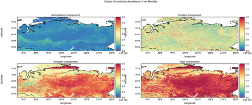
A breakdown of daytime 0.1 km daily and 0.1 km monthly maps has been provided to demonstrate the variability in uncertainty component propagation by region and by propagation scale. Breakdowns for two regions including the Amazon (Figure 2 and 3) and Australia (Figure 4 and 5) are presented here as examples of variations in uncertainty component propagation due to different surface types and processes. For all other regions including Western U.S.A., Greenland, Western Europe, Sahel, Siberia, China, and India please see Appendix A.

Figure 2. An uncertainty breakdown for the Amazon region, at 1 km daily on 15/7/2021. Highlighting the total error and the three components including atmosphere (water vapour), surface (emissivity) and random (noise).

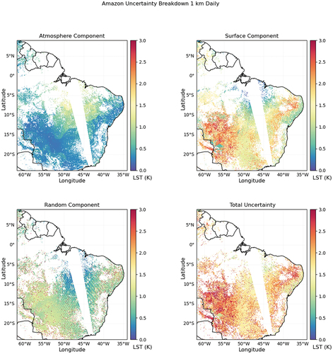
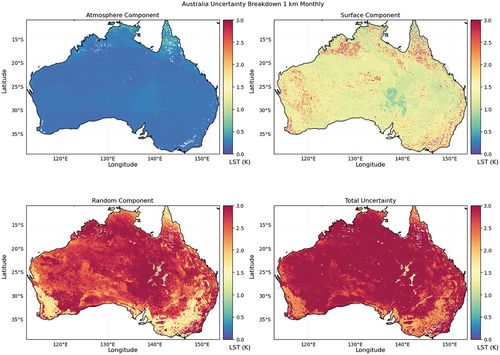
Figure 3. An uncertainty breakdown for the Amazon region, at 1 km monthly for July 2021. Highlighting the total error and the three components including atmosphere (water vapour), surface (emissivity) and random (noise and sampling uncertainty).

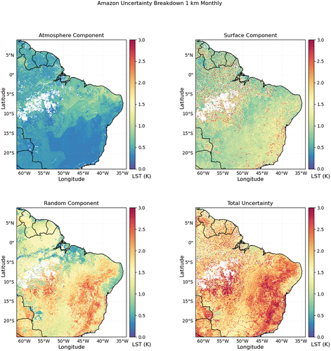
Figure 4. An uncertainty breakdown for Australia, at 1 km daily on 15/7/2021.Highlighting the total error and the three components including atmosphere (water vapour), surface (emissivity) and random (noise).

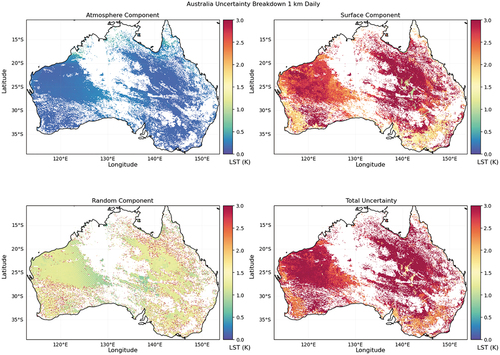
Figure 5. An uncertainty breakdown for Australia, at 1 km monthly for July 2021. Highlighting the total error and the three components including atmosphere (water vapour), surface (emissivity) and random (noise and sampling uncertainty).

Uncertainty propagation for the Amazon region at 1 km daily (Figure 2 and 1) km monthly (Figure 3) shows the total uncertainty, characterized by a relatively even distribution of the uncertainty components. This is mainly due to high atmospheric water vapour and surface homogeneity of vegetation and forests. The surface component has lower emissivity with small variations, typical of large closed canopies in the Amazon. These canopies contribute to a more homogeneous LST, reducing the LST variance and therefore the propagated sampling uncertainty.

Uncertainties for Australia demonstrate different dominant components at different propagation scales. Figure 4 shows how the daily total uncertainty is dominated by the surface component. Whereas, Figure 5 demonstrates how the monthly total uncertainty is dominated by the random component. Australia’s varying surface types of rocks, sands, and dry lands have higher emissivity uncertainties and therefore propagate as a larger sampling uncertainty within the random component on monthly scales. The random component dominance for Australia’s 1 km monthly uncertainties demonstrates how other components are reduced in propagation when LST variances are larger.

2.2.3. Statistical testing

Appropriate statistical testing was carried out to identify underlying patterns in the anomalies, as environmental data are often subject to autocorrelation. Autocorrelated data can lead to misrepresented associations between independent variables and reported trends (Ives et al. 2021; Weatherhead et al. 1998). Time – series analyses can present temporal autocorrelation when the values between time steps are not independent of seasonal signals and background noise, and therefore not statistically significant (Weatherhead, Stevermer, and Schwartz 2002). To account for potential autocorrelation, the Durbin–Watson test (Durbin and Watson 1950, 1951) was carried out on day and night-time anomalies for each ROI. The Durbin–Watson test determines a range between 0 and 4, where the accepted range between 1.5 and 2.5 considers the residuals having no autocorrelation (Draper and Smith 1998; Krämer 2011; Turner 2020). Trends were estimated using ordinary least – squares regression on the LST anomalies over the study period (Coolidge 2020). Cases where the Durbin–Watson score was <1.5 or >2.5, were indicative of autocorrelation and the gradient uncertainties were recalculated using the Newey–West estimator (Newey and West 1987). The maximum number of lags is identified by examining the autocorrelation function of the residuals, which were used to calculate the correct uncertainty and yield probability values (p–values) for each regional time series.

The p–values yielded from the fit were used to verify the observed anomaly climate trends. For this work, we consider a trend with a p – value <0.05 as statistically significant. The null hypothesis claims that observed changes between variables or in experimental results are due to chance and therefore hold no underlying trends or relationships. For this study, the null hypothesis is that there are no trends in the regional time series. A p–value <0.05 determines the null hypothesis should be rejected. A p–value >0.05 is considered not statistically significant, and the null hypothesis should be accepted. However, a p–value >0.05 does not determine whether there is no association or no evidence of a trend but is an indication that it may be less likely (Coolidge 2020; Whitley and Ball 2002).

3. Results

The following results describe anomaly time series and accompanying uncertainty analyses of the ROIs in Figure 1, initially for Western Europe. Western Europe was chosen as the test region following previous studies (Good et al. 2022) to reinforce confidence in the MYDCCI dataset. The other regions in Figure 1 were used to represent a range of biomes and for differential daytime – night-time warming. In general, the results show increasing day and night LST trends across Earth with uncertainty budgets consistently below 0.03 K. These low systematic uncertainties reflect a small seasonal cycle of the residual uncertainty variations (Ghent et al. 2019) and are consistent with our results for Western Europe test region, giving us confidence in our trend analyses.

Table 1 presents the day and night autocorrelation function, lag correction and p–values for each ROI. The results show how statistically likely the LST anomaly results could have occurred under the null hypothesis for each regional time series investigated between 2002 and 2021. Western U.S.A., Western Europe, Siberia, and India p–values are significant for both day and night-time. Both the Sahel and Australia p–values are significant for night-time and not significant for daytime, whereas the Amazon and China’s p–values are significant for daytime and not for night-time. Greenland’s p–values report both day and night-time as not significant.

Table 1. The p–values for each of the estimated trends in each region of interest. Where lag = 0, no autocorrelation was detected and the p–values were used as is, and where lag > 0, the p–values were corrected with the Newey–West estimator (Newey and West 1987), using the number of lags shown.p–values in bold are statistically significant.

Region	Daytime Lags	Daytime p-value	Nighttime Lags	Nighttime p-value
TheAmazon	3	0.001	6	.06
U.S.A.	4	0.005	0	0.0003
Greenland	1	0.3	0	0.4
Europe	2	0.006	3	0.0003
The Sahel	0	0.4	0	0.000000005
Siberia	2	0.0005	0	0.00001
China	1	0.0009	0	0.01
India	6	0.0009	0	0.0001
Australia	0	0.3	0	0.001

3.1. Test region

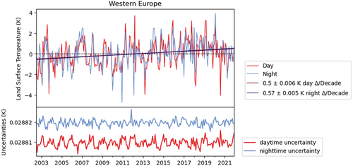
Good et al. (2022) proved the MYDCCI dataset is stable and provides a signal free from non – climatic discontinuities over Western Europe. Furthermore, we have used this region as our test area to give confidence in the data and our results. Western Europe’s day- and night-time anomalies demonstrate a large seasonal cycle with overall increasing temperature trends, with both time series increasing by +0.5 K and +0.57 K per decade. This is similar to the results in Good et al. (2022) who derive equivalent warmings at matched satellite and in situ locations; results for day (Tmax) and night-time (Tmin) were +0.65 K and +0.67 K for satellite and +0.52 and +0.59 for in situ, respectively. Large warm and cold anomalies can be observed over the study period, reaching minimum and maximum temperatures of less than −4 K and more than +3 K for both day and night, respectively. The night-time trend peaks are slightly larger than the day, until 2013 when minimum temperatures are much warmer staying above −2.5 K. Daytime anomalies have a sharper increase between 2004 and 2006, rising from −2 K to around +1 K and then again during a warm phase between 2006 and 2007 where they stay well above 0 K. After 2013, both trends rise steadily to where temperatures drop below 0 K less frequently between 2018 and 2020. The uncertainties exhibit a stable, seasonal cycle for Western Europe LSTs. Daytime results are consistently lower, whereas the night-time uncertainties are higher, peaking in November 2011. Although, a larger variance in anomalies can be observed throughout the year during the day than at night.

Western Europe’s annual temperature cycle shown in Figure 6 suggests strong seasonality, with oscillations of warm and cool anomalies ranging up to +7 K. The region’s significant day and night-time p–values where p < 0.05 (Table 1) reject the null hypothesis, supporting the alternative hypothesis that Western Europe’s time-series trends are climate – related. We can infer from Good et al. (2022) study that our warming trend per decade is close to 0.6 K and therefore consistent with their reported in situ trends. Furthermore, our results for Western Europe agree with previous studies, suggesting that we can expect the daytime trend to be close to the night-time trend (Cox et al. 2020). The LST trends for Western Europe are indicative of large – scale atmospheric circulation influences. Jones and Lister (2009) found atmospheric circulation dominant on climatic forcing of surface temperatures and its seasonality. Regional climate model projections stipulate positive feedback influences of systems such as the North Atlantic Oscillation (NAO) (Kjellström et al. 2013). Europe presents relatively stable seasonal uncertainty cycles compared to other ROIs, albeit more variable for the daytime than the night-time. Furthermore, it is likely that climate drivers rather than land – use change are the reason for the uncertainty cycles and general LST anomaly increases. Drought is a significant natural hazard, especially in Europe, that is intensified as a result of anthropogenic global warming. Climate models determine Europe as a key area for hydro – climatic change, as a result (Gudmundsson and Seneviratne 2016). Strong correlations between Europe’s seasonal temperature and precipitation, with drought events, have been well – documented (Hurrell 1995; Luterbacher et al. 2004). Hellings and Rienow (2021) argue the effects of urbanization on UHI intensification. Highlighting that both warming – induced heatwave frequency and European city developments influence the surface temperatures. The 2003 record-breaking European heatwave was one of the many extreme weather events caused by global warming. It caused an estimated mortality rate of more than 70,000 people, forest fires particularly in Portugal from arid conditions, and reductions in river and reservoir levels (MetOffice 2019). García-Herrera et al. (2010) suggested the NAO and social moisture deficit were key factors for the unprecedented surface temperatures in 2003. Furthermore, it is in agreement with Western Europe’s results showing warm anomaly events of 2003, 2010, and 2018 (Figure 6). Recent studies (Liu, Hagan, and Liu 2020) suggest all three heatwaves were induced by atmospheric circulation anomalies. The 2003 and 2010 events were enhanced by moisture – temperature coupling, and 2018 was due to surplus net surface radiation associated with reduced precipitation. Regional climate models suggest surface temperatures are projected to increase across Europe (Carvalho, Cardoso Pereira, and Rocha 2021), changing climate drivers and increasing the likelihood of the intensity and frequency of droughts and heatwaves (Gouveia et al. 2022).

Figure 6. MYDCCI day and night LST anomalies with gradient uncertainty, and accompanying propagated uncertainty budget for West Europe region between 2002 and 2021.

3.2. Other regions of interest

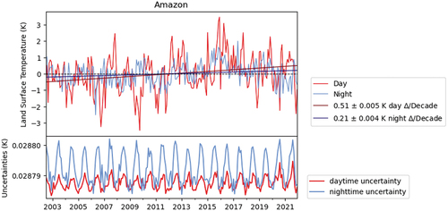
LST anomalies for the Amazon region (Figure 7) in general exhibit a stable, seasonal cycle from 2002 to 2013. Daytime LSTs vary between −2 K and +1 K, with cold anomaly events in 2006 and 2009 of < −3 K. Although the daytime displays a large seasonal cycle, warm anomaly spikes only reach +2.5 K once before 2008. Nighttime trends appear to be more stable with a smaller seasonal cycle, where the minimum temperature stays above −2 K except for January 2006 whereafter the occurrence of warm anomalies increases from 2012 and anomalies greater than +3 K occur in 2015. A steep rise in temperatures showing a four – year warm period occurs for both day and night between 2014 and 2018, where minimum cold and maximum warm anomalies stay above −1.5 K and reach almost +4 K, respectively. Thereafter, an apparent cooling occurs for both day- and night-time anomalies, most prominently with the former. However, the overall trend analysis shows an increase in LSTs, with a change of +0.51 K (daytime) and +0.21 K (night-time) per decade. Conversely, the night-time uncertainties demonstrate a much larger seasonal cycle, peaking in June 2007. This suggests increased uncertainty during the summer months for the Amazon region. Daytime uncertainties are lower and fairly stable, suggesting less doubt about the correlating temperature anomaly results. However, uncertainties increase towards the latter end of the time series.

Figure 7. MYDCCI day and night LST anomalies with gradient uncertainty, and accompanying propagated uncertainty budget for the Amazon region between 2002 and 2021.

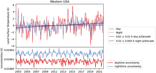
Western U.S.A. LST anomalies (Figure 8) suggest a clear and consistent significant temperature increase over the study period, with a + 0.82 K and +0.52 K change per decade for both day and night, respectively. It is evident that both trends vary similarly, exhibiting regular, large cold, and warm events. Daytime anomalies vary more in comparison to the night-time over two decades, between low and high peaks of almost −6 K and +6 K. Night-time anomalies during this period follow this trend also, although peak temperatures are lower with lesser variation between −4 K and +4 K. Temperatures for both day and night stay consistently above −4 K post–2013, except for two significant daytime cold anomalies of up to −6 K towards the end of 2018. Both temperatures show a steep rise and stay above −3 K until the end of the study period. Similarly, the day- and night-time uncertainties also reflect a stable, seasonal trend. The latter demonstrated slightly higher uncertainties than the former, peaking in February 2012.

Figure 8. MYDCCI day and night LST anomalies with gradient uncertainty, and accompanying propagated uncertainty budget for West U.S.A. region between 2002 and 2021.

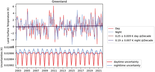
Figure 9 demonstrates the anomalies and uncertainty budget for Greenland over the study period. Overall, the day- and night-time anomalies exhibit a relatively stable, but overall increasing trend for day and night with a change per decade of +0.25 K and +0.19 K, respectively. Both agree with each other well, exhibiting clear, strong seasonal oscillations. Warmer LSTs can be observed from 2002, with high minimum temperatures ranging above −1 K. A significant, sharp increase occurs between 2009 and 2012. Where a cold anomaly of −3.9 K towards the end of 2009 rises to almost +5 K by January 2010. Temperatures stay above 0 K for more than a year, whilst also recording its highest daytime LST of more than +6 K, before dropping to less than −4 K by 2011. Both day and night anomalies fall back into a more stabilized, cooler phase before average temperatures are observed to rise and stay above −2 K in 2021. Greenland’s uncertainties show large day and night-time variations. The daytime values are consistently lower, characterized by large negative spikes, reaching a minimum in December 2013. The two – time series agree that in general, higher uncertainties occur during the summer months and are lower in the winter.

Figure 9. MYDCCI day and night LST anomalies with gradient uncertainty, and accompanying propagated uncertainty budget for Greenland between 2002 and 2021.

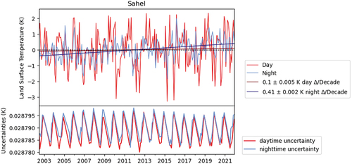
Although LST anomalies for the Sahel (Figure 10) generally agree on a seasonal scale, the daytime displays larger oscillations compared to the night-time. Furthermore, the daytime appears more stable over the time period with only a + 0.1 K change per decade, as opposed to night-time +0.41 K change per decade. Daytime minimum and maximum peak anomalies are more extreme. With minimums of almost −3.5 K between 2015 and 2016 and maximums consistently over +2 K from 2009. Nighttime anomalies, however, never reach a minimum of less than −2 K and rarely reaches a maximum of +2 K other than in 2016. They appear to steadily increase over time, with some longer periods of warming between 2007 and 2010 and again between 2012 and 2016. The uncertainties exhibit a strong seasonal cycle for the Sahel that is almost identical for both day and night, both peaking in December 2011. Uncertainties are much lower during the summer months and appear to be higher in the winter, with little deviation over the whole study period.

Figure 10. MYDCCI day and night LST anomalies with gradient uncertainty, and accompanying propagated uncertainty budget for the Sahel region between 2002 and 2021.

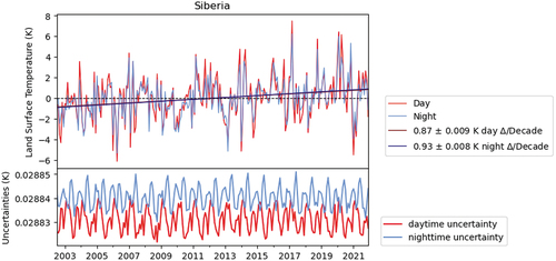
The region of central Siberia (Figure 11) shows a significantly increased day and night LST change per decade of +0.87 K and +0.93 K, respectively. Day- and night-time agree with a clear seasonal cycle and present a series of warm and cold anomalies between +8 K and −6 K, respectively. For a period between 2007 and 2011, anomalies appear relatively stable and cool between −4 K and less than +2 K. Temperatures are relatively stable with shallow oscillations where night-time is more variable than the day, and an overall increasing trend. However, the results show a few large oscillations during periods between 2006 and 2007, 2012 and 2014, 2016 and 2017, and 2019 and 2020. The uncertainties reveal a large seasonal cycle, where night-time is higher than daytime, peaking in June 2017. The results suggest much lower uncertainties during the summer seasons compared to the winter months.

Figure 11. MYDCCI day and night LST anomalies with gradient uncertainty, and accompanying propagated uncertainty budget for the central Siberia region between 2002 and 2021.

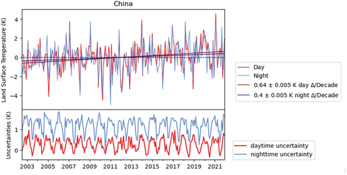
Figure 12 demonstrates a significant day and night LST anomaly increase over the study period for China, with change per decade of +0.64 K and +0.4 K, respectively. Both time series agree well, although night-time appears to have a larger variance between cold and warm anomaly events. Up until 2011, cold anomalies regularly reach or surpass −4 K for both day and night. However, thereafter, it is clear that the minimum anomaly threshold is much warmer and does not reach +4 K. In agreement with this, warm anomalies are more prominent after 2013, with three events surpassing +2 K in 2013, 2019, and 2020. Overall the night-time appears more stable, as apparent by the much lower rate of change per decade. In comparison, the daytime anomalies rise consistently, presenting much warmer daily temperatures over time. The night-time uncertainties presented for China are higher, peaking in February 2006, and have a larger seasonal variation compared with the daytime. The daytime maximum agrees with night-time minimum uncertainties, peaking in March 2003. Both time series, however, follow a seasonal cycle that demonstrates lower uncertainties towards the spring and summer months.

Figure 12. MYDCCI day and night LST anomalies with gradient uncertainty, and accompanying propagated uncertainty budget for China between 2002 and 2021.

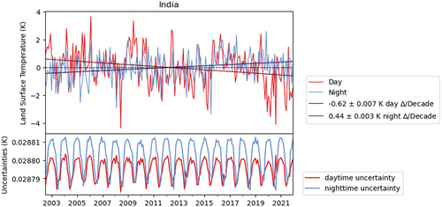
Figure 13 shows an anomalous cooling daytime change per decade of −0.62 K, compared with a positive night-time trend of +0.44 K for India. Both time series show seasonal synchronicity, with more extreme daytime warm and cool anomalies. Temperatures present an upward trend between 2002 and 2007 before a large mid – season cold anomaly of less than −4 K in 2008. Warm anomalies at or above +2 K occur thereafter until temperatures stabilize between 2010 and 2016. A decreasing daytime trend is observed from 2017 with a phase of significant cold anomalies from 2019. The night-time trend generally follows this pattern, but the anomalies are more stable, with temperatures staying between −3 and +3 K for the whole study period. Both uncertainty trends show significant seasonal cycles, with higher uncertainties during winter, where day and night-time peak in February 2004 and January 2006, respectively. Night-time uncertainties are higher than the daytime; however, negative spikes characterize the daytime. Furthermore, daytime presents more of an oscillating seasonal trend over the winter.

Figure 13. MYDCCI day and night LST anomalies with gradient uncertainty, and accompanying propagated uncertainty budget for India between 2002 and 2021.

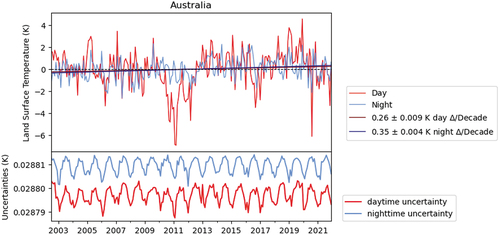
Figure 14 presents Australia’s LST anomalies that demonstrate more variation in warm and cold extremes as opposed to overall temperature increase. The night-time increased more per decade than during the daytime, by +0.35 K compared to +0.26 K, respectively. However, the daytime anomalies show larger oscillations. 2002 to 2010 appear relatively stable for both time series; however, a large drop from 0 K to almost −8 K occurs between 2010 and 2011. This cold event lasts around 2 years before daytime temperatures re–stabilize and is most likely affected by the daytime LST change per decade. Night-time cold and warm anomalies stay between −3 K and +2.5 K for the entire study period. Contrary to this, Australia’s day and night-time uncertainties agree with a stable, seasonal cycle. Although the daytime uncertainties are lower than at night. Both series show increased uncertainty during the summer months, peaking in July 2002 and in August 2016, respectively.

Figure 14. MYDCCI day and night LST anomalies with gradient uncertainty, and accompanying propagated uncertainty budget for Australia between 2002 and 2021.

4. Discussion

4.1. Land surface temperature trends

The Intergovernmental Panel on Climate Change (IPCC) 2022 stated that the global surface temperature between 2011 and 2020 is 1.09°C higher than the 1850–1900 threshold (Arias et al. 2021). Highlighting the significance of global warming and the need for regional LST analyses using robust climate data and uncertainties such as MYDCCI. While knowledge of global LST temperature is imperative for understanding Earth’s energy budget, different regions respond to climate change in various ways, so regional analyses are key to identifying changing patterns. In general, all ROIs in this study (Figure 1), other than India, show statistically significant positive trends in day and night-time LSTs between 2002 and 2021 for MYDCCI. All regions show evidence of seasonal variations, but each region presents different trends associated with its climatic characteristics. Some regions, such as Siberia, the Amazon, Western U.S.A., Greenland, and China, show significant daytime temperature trend increases over the two decades studied, as demonstrated by the most significant daytime changes per decade, of +0.87 K and +0.82 K for Siberia and Western U.S.A. respectively. Both regions also show some of the largest night-time anomaly trends, although Siberia dominates with the topmost change of +0.93 K. Similarly to Siberia, Australia, and Sahel’s night-time trends exceed their daytime by +0.9 K and +0.40 K, respectively. Conversely, India is the only region displaying a decreasing daytime trend of −0.62 K, but an increasing night-time trend of +0.44 K per decade. China presents a significant, positive daytime trend of +0.64 K per decade, which is not mirrored by its night-time trend of only +0.4 K per decade. A steadier rise in temperatures is observed in Greenland, with a day and night-time change per decade of just +0.25 K and +0.19 K, respectively. Although its time series displays one of the largest anomaly increases of more than +8 K in 2010.

4.2. Regional analysis

4.2.1. The Amazon

The Amazon has been found to show a significant temperature increase in day and night-time trends, with a change per decade of +0.51 K and +0.21 K, respectively. High night-time uncertainties may be a result of cloud cover, where cloud contamination is higher at night, impacting the scene variance and furthering the sampling uncertainty. Low daytime uncertainties reinforce the rising anomaly results for the Amazon, as one of the fastest warming ROIs. Daytime trends appear to be statistically significant (p < 0.05), while the night-time time series is too noisy for a trend to be reliably estimated in this work (p > 0.05). Previous research from modelling and observational studies suggest a significant influence of tropical forest deforestation on local and regional LSTs (Lawrence and Vandecar 2015). Climate modelling studies found that Amazonian deforestation causing biogeophysical effects is likely to increase surface temperatures and alter precipitation and climatic patterns locally (Lejeune et al. 2015). Land use transitions from native vegetation of natural forests and savannah to pastureland due to agricultural expansion can lead to a drier and warmer local climate (Swann et al. 2015). Satellite observations reveal how surface temperature increases as evapotranspiration reduces, especially during the dry seasons. The effects of which create positive feedback on the water cycle and atmospheric energy budget on a microscale (Lawrence and Vandecar 2015). Evidence (Swann et al. 2015) suggests the significant temperature increase in 2015 in Figure 7 can be attributed to an extreme drought associated with El Niño Southern Oscillation (ENSO). ENSO is a key large – scale oceanic system that influences atmospheric pressure fronts of sea surface trade winds affecting the Amazonian climate. The intensification of ENSO events is a by – product of global warming and is linked to two extreme drought events (Jiménez-Muñoz et al. 2013). The day and night warm anomaly jump observed in 2005, 2010 and 2015; may be attributed to three droughts associated with ENSO, and its effect on forest mortality due to water stress (Jiménez-Muñoz et al. 2013). The MYDCCI LST anomaly and uncertainty results, therefore, suggest Amazonian temperatures are rising, supporting evidence of the significant feedback effects of land – use change and global warming.

4.2.2. Western U.S.A

We have found evidence of significant recent LST change for Western U.S.A. (8), with the topmost day and night change per decade of +0.82 K and +0.52 K, respectively. Table 1 shows that both day- and night-time trends are statistically significant for this region p < 0.05, supporting the rejection of the null hypothesis. Studies suggest two key drivers of this could include the influence of atmosphere – ocean systems, agricultural production, and urban development, and an increase in extreme weather like droughts. The Pacific Decadal Oscillation (PDO), similarly to that of ENSO, involves air – ocean interaction which affects Western Pacific climate variability (Mantua and Hare 2002). Yan et al. (2020) found a strong – positive correlation between PDO and LST seasonal variations in North – West America, however, state that the overall influence on LST is small. Their study also discussed the effect of the region’s complex geographical environment and its individual influence on regional LST, including the economic development and wildfire intensity of the arid west coast peninsula of California. Air currents from the cold Arctic and from the warm Gulf of Mexico are channelled through the alpine coastal mountains of the Sierra Nevada, which have an impact on land change and heatwave events on the array of tropical glaciers and river basins within the western mid – latitudes. Although many factors may influence West American LST, it is well documented that increases in extreme weather events and their spatio-temporal variability are major causes of rising temperatures (Kogan and Guo 2015; Wan, Wang, and Li 2010). As seen in Figure 8, 2006, 2012, and 2014–2015 saw steep temperature rises. Kogan et al. (2015) suggested the multi-year mega – drought from a strong ENSO event caused severe eco – stress and significantly affected regional LSTs. Rippey (2015) attributed a record-breaking 2012 drought to severe air temperatures and agricultural land damage. Recent studies (Leeper et al. 2022; Yan et al. 2020) corroborate our results which suggest that the Western U.S.A. suffered a severe drought in 2015, as demonstrated by a significant rise in the day and night-time anomalies. Although drought events driven by extreme weather seem to be the driving force of recently increasing LSTs, the complexity of regional climate phenomena and the variety of land surface classifications may increase uncertainties in quantifying Western U.S.A.’s LST trends.

4.2.3. Greenland

For this paper, the Greenland ice sheet’s (GrIS), ice surface temperature (IST) is generalized as LST. Table 1 shows that the day and night-time trends are not significant where p > 0.01 and therefore supports the null hypothesis that Greenland’s trends are less likely to be related to climate change. A key reason for this may be attributed to the susceptibility of cloud contamination in the data, due to the variability of atmospheric circulation systems. Land – atmosphere dynamics are a huge influence on Greenland’s climate, and its variability can be greater than the underlying changes. Furthermore, the MYDCCI dataset has a relatively short time span of data acquisition, which may affect the p–values results for Greenland and all other ROIs. Although the p–values reflect that the results are unlikely to be due to a climate trend, Greenland’s time series may, however, be a result of natural variability. The importance of Arctic amplification and near – surface air temperatures (T2m) are well documented and understood, especially in Greenland. However, its relationship with LSTs is less understood due to the poor understanding of uncertainties and issues with clear – sky bias associated with TIR retrievals (Hofer et al. 2019). This is demonstrated in Figure 9, as the negative daytime uncertainties suggest a lack of data. Day and night anomalies increase over time; however, the results are dominated by noisy oscillations.

In particular, 2002 to 2006, 2009 to 2012, 2015 to 2017, and 2020 to 2021 saw steep jumps from cold to warm anomalies. Hall et al. (2006) demonstrated that during the melt – season of 2002 to 2005, GrISs surface temperatures were at their highest compared to a six – year mean. The likely result of surface dry – snow reduction and instability related to rising T2m. These surface changes reduce the albedo effect and create a positive feedback mechanism to further cause temperature rises and extreme melt events. By utilizing remote sensing techniques, we are able to identify large – scale features that characterize Greenland’s climate and therefore subsequent processes and feedbacks of its surface. For example, Figure 9 shows a significant positive temperature anomaly between 2010 and 2012. Evidence suggests that within this period positive temperature spikes were driving forces for severe melting, which have been linked to impacts like increased melt – water discharge in Kangerlussuaq (Van as et al. 2012), ice shelf calving of the Petermann Gletscher (Nick et al. 2012) and interior ice velocity acceleration (Doyle et al. 2014) across Greenland. Although the direct links between global warming and surface – related feedbacks are well researched; evidence also suggests that natural ocean – atmospheric systems such as the Greenland Blocking Index (GBI) and the NAO significantly influence surface temperatures and changes. High – pressure anti – cyclonic blocking of mean 500 hPa geopotential height that amplifies the Northern Polar jet – stream flow, known as the GBI, has been linked to influencing enhanced warm periods over Greenland (Hanna et al. 2016). GBI has been coupled with the NAO index, a large – scale dipolar oscillation in surface pressure between the low – pressure North Atlantic and high – pressure mid – latitude (Davini et al. 2012). Both systems oscillate between cold and warm phases, which correlates with the seasonal oscillations in Figure 9. Furthermore, an extreme NAO event in 2010 (Barrett et al. 2020) would likely explain the substantial increase of more than +8 K between 2010 and 2012.

4.2.4. The Sahel

Results from the semiarid region of Sahel (Figure 10) shows a more noisy trend of temperature increase, more so at night in comparison with other ROIs. The uncertainties also depict much larger, seasonally dominated variances for both day and night LSTs. Table 1 shows the Sahel’s p–values as not significant where p > 0.01 and significant where p < 0.05 for day and night-time, respectively. The p–values suggest the results are not related to a climate trend for the daytime, but the null hypothesis can be rejected for the night-time. The uncertainty and daytime p–value results are most likely due to Sahelian climatic characteristics involving its wet season, which occurs from its transition between the arid Sahara to the north and the tropical rain – forest to the south (Epule et al. 2014). This could lead to cloud misinterpretation from less clear – sky TIR observations, which may explain why the Sahel’s uncertainties are nosier and the daytime anomalies p–value are not significant.

The influence of the Hadley cell, a low – latitude atmospheric system of over – turning circulations responsible for tropical trade winds, exerts control on regional weather patterns. This results in a highly variable rainfall distribution associated with the intertropical convergence zone (ITCZ) (Rodríguez-Fonseca et al. 2015). This might explain the noisy oscillations and clear seasonal influence on LST anomalies in 10. Studies demonstrate the dominance of precipitation patterns that are connected to the West African Monsoon (WAM), which impact the surface energy balance (Biasutti 2019). This is a process primarily due to variability in evaporation from vegetation changes affecting surface fluxes and warming rates (De Kauwe et al. 2013). Surface temperature changes in this region are still widely debated. Furthermore, research has linked the radiative forcing of desert dust, variable remote SSTs, and changing surface conditions to extensive droughts and desertification. Yoshioka et al. (2007) used general circulation model simulations to find atmospheric forcing and feedbacks of dust that may account for rainfall reductions. Further leading to prolonged dry seasons, drier soils, and water – limited plants which might impact surface temperatures. However, Epule et al. (2014) challenges the lack of quantification in the role of dust and land – use change and further discuss how global warming feedbacks are the main driving factor of droughts and surface temperature changes seen in Figure 10. Most research recognizes the influence of SST on Sahel’s variable climate and supports the surface changes and the increasing trend seen in our results. Lu (2009) suggested Indian Ocean SST warming to surface dynamic changes from increased radiative forcing, to intensified Sahelian droughts that are a key climatic event affecting the Sahel. Similarly, Rodríguez-Fonseca et al. (2015) discussed the links between anthropologically – induced SST warming and enhanced ENSO events, to increased local convection in West Africa, which is linked with rising surface temperatures. In agreement, Biasutti (2019) hypothesized the role of rising SSTs, rainfall anomalies, and WAM variability to inter – hemispheric aerosol loading and increased greenhouse gas emissions. Although the nature of the Sahelian climate is variable and therefore widely debated, it is likely that more than one factor may impact key climate characteristics and seasonalities responsible for the changes in Sahel’s LSTs which are observed over the past two decades.

4.2.5. Siberia

The most substantial increase in LSTs over the study period was found in Siberia 11, with significant temperature change per decade for day and night-time of +0.87 K and +0.93 K, respectively. The day and night-time uncertainties are generally in agreement and are characterized by a strong seasonal cycle. With lower uncertainties during the summer, and some variability towards December and January. Table 1 suggests that we can reject the null hypothesis, as both day and night-time p–values were p < 0.05, is significant and supports that Siberia’s anomaly results are climate trends. Lu, Zhang, and Guan (2022) have linked the influence of more frequent Northern Hemispheric extreme cold events under global warming, to colder – than usual winter anomalies. Winter anticyclones and large – scale atmospheric circulations such as the Siberian High affect energy dispersion and cool temperatures. Furthermore, these synoptic – scale systems driven by Eurasian atmospheric patterns have also been closely linked to Siberian seasonal anomalies (Lu 2017; Röthlisberger et al. 2019). This is in line with the results; showing a clear seasonal cycle, with several cold anomalies becoming more frequent during the latter half of the last decade, especially in 2006, 2012, 2013, and 2020. It is suggested (Muster et al. 2015) that local and regional surface energy regimes are the main influence of Siberian surface temperature trends, which are enhanced by Arctic amplification and increased global warming. It has been well documented (Hinzman et al. 2005; Langer et al. 2011; Serreze et al. 2000) that Siberia has already been impacted by climate change and permafrost holds a dominant role over its surface properties. This is in line with Figure 11 and may be linked to the substantial temperature trend increase over the last two decades. Regions with significant permafrost properties, such as Siberia, are particularly at risk of thawing and inducing positive climate feedbacks (Yoshikawa and Hinzman 2003). Moreover, Siberian land cover changes affect a variety of biogeophysical properties that influence the surface energy balance including emissivity, surface roughness and moisture on latent and sensible heat fluxes (Hinzman et al. 2013). In line with this, associated weather patterns and increased extreme precipitation events in Siberia have also been positively linked to permafrost and subsequent surface warming (Wang et al. 2021). The scarcity of surface observations and the complexity of surface fluxes in Siberia make it difficult to fully comprehend the surface processes affecting LST changes (Wang et al. 2021). However, these recent studies highlight the role of climate forcing on permafrost and surface properties, which are linked to the significant warming LST trends in our results.

4.2.6. China

Remote sensing and reanalysis research indicates consistent warming trends of LST based on a variety of spatial and temporal scales. China’s p–values (Table 1) are significant, p < 0.05, and not significant, p > 0.05, for day and night-time, respectively. This suggests that the null hypothesis can be rejected, but that daytime is more likely to be due to climate trends compared to the night-time. China’s anomaly results for 12 show a higher daytime temperature trend change than night-time of +0.64 K and +0.4 K, respectively, characterized by seasonal uncertainty cycles showing higher uncertainties throughout the winter. Research suggests this may be due to a combination of global warming and heat retention from the effects of urbanization (Song et al. 2018) Song et al (2021) recently found strong relationships between rising air temperatures and LSTs between 2003 and 2019. Furthermore, evidence of vegetation coverage, albedo, and evapotranspiration was linked to driving LST changes in China (Xiao et al. 2008). Coupled rising air and surface temperatures, however, are further impacted by land – use and land – cover changes in rapidly developing regions or mega – cities such as Beijing, Shanghai, Guangzhou, and Taiyuan. As a result of China’s substantial urban growth, surfaces, and landscape changes affect the local radiative, thermal, moisture, and aerodynamic properties. Furthermore, the spatial heterogeneity between day and night on annual and seasonal LSTs characterized by UHIs (Geng et al. 2022) is in line with the results in Figure 12. Liu et al. (2018) discussed the formation of urban agglomerations in China, where the UHI effect is now causing rising surface temperatures over larger regions rather than being limited to a city. This is reflected in Figure 12, but especially noticeable towards the end of the study period between 2013 and 2021. Duan et al. (2019) found a direct link between rising surface temperatures in Taiyuan and increased impervious surface areas. Research into Beijing’s UHI growth by Xiao et al. (2008); found strong correlations between higher LSTs and increased built – up areas, compared to lower LSTs of forests and farmlands. The effects of city UHIs are just one issue when understanding China’s surface temperature change. More than half the country is covered by arid and semiarid regions, which have suffered environmental changes due to desertification, grassland degradation, and intensified warming. These also have effects on surface energy balances, precipitation patterns, and susceptibility to drought (Chen et al. 2011). Evidence suggests that the anomalous changes observed in Figure 12 can therefore be directly linked with rapid urbanization and tropospheric warming with minimal uncertainty. Further, influencing positive feedbacks that critically drive further climate change (Jia et al. 2022). This research supports the significantly increasing trend in Figure 12.

4.2.7. India

India’s results present a negative daytime, as opposed to positive night-time, temperature change per decade. Furthermore, Table 1 reflects significant p–values, where p < 0.05 for day and night-time for India. This rejects the null hypothesis, and it supports that India’s anomaly results are attributed to climate influence. The daytime trend suggests surface cooling over the study period, with a seasonal cycle of low, negative uncertainties during the summer (Figure 13). Changes in surface temperatures may be attributed to feedbacks from the Indian summer monsoons (ISM) between June and September. Monsoon circulations have been linked to aerosol solar absorption and a rise in summer rainfall (Gautam et al. 2009). Analyses reveal that increased anthropogenic emissions over Asia have led to cooling since the 1970s. Sulphur dioxide (SO₂) emissions across the South Asian region have more than doubled since 1970. Aerosol loading, known as the South Asian haze, builds up over winter and leads to a decrease in clear – sky daily radiative surface heating (Krishnan and Ramanathan 2002). The effects of aerosols may impact cloud masking and could potentially be linked to the discrepancies between day- and night-time anomalies (Figure 13). More recent studies (Ross et al. 2018) further corroborate the effect over India and find that warming of the haze leads to surface air cooling underneath. However, Katzenberger et al. (2021) highlight the declining cooling effect of aerosols is due to policy implementations and increasing ISM rainfall patterns may be dominant. It is a possibility that cloud – masking may affect how aerosols are detected between day and night, providing a possible reason for discrepancies over the diurnal cycle in the results. Changes in the ISM seasons have led to an increase in rainfall over India as a result of tropospheric land – sea thermal gradient strengthening (Gautam et al. 2009). Monsoon depressions and low – pressure areas have been found to influence significant, widespread rainfall over central India (Hunt and Fletcher 2019). The increased rainfall during the IMS has been linked to regional surface cooling from feedbacks between the atmosphere and land (Gautam et al. 2009). Furthermore, Jin and Wang (2017) related increasing lower tropospheric meridional temperature gradients to warming LST signatures, which intensify the Hadley circulation and subsequent monsoon rainfall. Consistent increases in monsoon rainfall from global warming have also been found in studies using global climate models within the Coupled Model Intercomparison Project Phase 6 (CMIP6). Where 32 models show significant increases in monsoon precipitation and will continue to do so under 21st – century climate change projections (Katzenberger et al. 2021). Basha et al. (2017) found Indian LST changes per decade increased by +0.055 K between 1860 and 2005 and their analysis of CMIP Phase 5 (CMIP5) projections of a warming surface temperature trend during the twenty-first Century for India, are in line with our results. During the ISM, Deshpande, Kulkarni, and Krishna Kumar (2012) found 60% of precipitation fell during the day in north – central India, which supports the diurnal temperature discrepancies of recent daytime summer cooling in our results. Moreover, above – normal precipitation was correlated with a severe ISM season within the last 3 years due to the strongest, positive Indian Ocean Dipole (IOD) event on record (Ratna et al. 2021). This may explain why Figure 13 shows a larger anomalous cooling period of daytime temperatures in recent years, as opposed to minor cold anomalies earlier in the timeline.

4.2.8. Australia

Results in Figure 14 for Australia show a surface temperature pattern over the past two decades. Table 1 depicts p–values for Australia. The daytime trend is not significant, where p > 0.05, but the night-time is significant, where p < 0.05. The rejection of the null hypothesis for the daytime is likely due to issues with cloud contamination related to the variability of wet seasonal events such as La Niña. Whereas, the night-time p–values suggest Australia’s night-time anomalies represent a climate trend. Higher uncertainties can be observed towards the summer for both day and night, which correspond to the effects of Australia’s variable wet season. Over the last couple of decades, observations of Australia’s climate suggest wetter summers, although overall temperatures continue to increase. Modelled surface energy budgets emphasize the effects of the summer monsoons and large – scale circulations, like ENSO, on the continents’ sensitivity to climate extremes (Wardle and Smith 2004). Recent studies (Yu and Notaro 2020) suggest how land surface feedbacks including vegetation and soil moisture affect regional climate variability. It has been found that the Madden – Julian Oscillation (MJO), a large – scale tropical atmospheric circulation that presents as atypical rainfall patterns, contributes to climate feedbacks. Previous modelling and observations (Risbey et al. 2009; Wheeler et al. 2009) have determined that the MJO significantly influences Australian monsoon rainfall and supports the seasonal anomaly oscillations in our results. Other large – scale ocean – atmospheric systems, including the Interdecadal Pacific Oscillation (IPO), the Southern Oscillation Index (SOI), and ENSO, have been linked to rainfall patterns. All of which are characterized by the Walker Circulation, a result of differences in heat and moisture distribution between the ocean and land (Heidemann et al. 2022). Furthermore, the ‘see-saw’ interactions can alter the regional climate and subsequent surface temperatures. La Niña, the counterpart to ENSO, is a period where SSTs across the eastern Pacific Ocean are below average and affect regional weather patterns (Yoo et al. 2010). 2010 and 2011, saw one of the strongest La Niña events on record and brought extensive precipitation to Australia (Evans and Boyer-Souchet 2012). In line with this, Figure 14 depicts large negative LST anomalies between 2010 and 2012. The winter of 2010 saw rainfall rates more than 21% above average, alongside negative outgoing long – wave radiation anomalies indicative of strong convection and cooling (Ganter 2011). This is a key example of how remote sensing can highlight coherent features in time, which are likely the best regional characterization of large – scale changes such as evidence of regional air – ocean climate system forcing on surface temperatures in Australia.

5. Conclusions

This study highlights the importance of LST and satellite observations for monitoring surface temperature trend variability, the Earth’s energy budget, and its response to global warming. We used Western Europe as a test region, to verify and demonstrate the value and robustness of the MYDCCI dataset for trend analysis of eight regions of interest. It is shown that, using current expressions of uncertainty in LST datasets, large regions can be addressed where the total uncertainties are dominated by residual systematic biases in LST anomaly space. Most significantly, our findings reveal substantial LST trend increases for Siberia and the Amazon, with recent increases in LST trends for Western U.S.A. The p–value results suggest that most ROI time series are significant and therefore are statistically likely to reflect climate trends. However, Greenland, the Sahel, China, the Amazon, and Australia have either one or both p–values that are less than or not significant. This means that the derived anomaly trends are valid for these regions but are not significantly different from zero; so either climate change effects are small or mitigated by other landscape changes. The anomaly results clearly show rising day and night LST trends for all regions other than an atypical daytime trend, for India, with low uncertainties reinforcing confidence in trend analysis. This general behaviour is in line with the IPCC’s report (Arias et al. 2021) of rising surface temperature. Perhaps as important, our analyses have highlighted how remote sensing of LSTs can identify and characterize regional climates, having identified coherent anomalous periods of warming and cooling in Greenland and Australia, which are as important as trends whether they are changing multi – annual regional regimes or extreme weather events. Our results have clearly shown that large regions are best suited to current climate analyses of LST change and trends because of the increased importance of random errors at high spatial resolutions; both noise and sampling uncertainties are increased. Further studies could usefully be undertaken at point locations or for small regions with a focus on testing the assumptions about correlations of uncertainties where there may be co-dependencies. In addition, it would be very useful to identify additional biomes of regions where LST trends can be tested against other biomes to give confidence in derived trends and also to look at interdependencies with other land, atmosphere and water variables. The continuing operation of long-term LST sensors such as SLSTR, MODIS and Landsat offers increasing prospects for an LST climate analysis which is able to capture the size of change over the next two critical decades of greenhouse gas-induced warming.

Open research

The satellite LST data used in this study are provided by the LST_cci project. Official versions of these datasets are freely available via the ESA Open Data Portal (https://climate.esa.int/en/odp/#/dashboard). The data and software presented in this study are not publicly available yet due to privacy and legal concerns but are available on request from the corresponding author.

Acknowledgements

Abigail Waring would like to thank the University of Leicester's Physics and Earth Observation Science departments for the opportunity to conduct research through a PhD. To the first supervisor Dr Darren Ghent for his patience and guidance during her PhD research and learning. To the surface temperature research team for their support; Dr Mike Perry, Dr Jasdeep Anand, Dr Karen Veal and Professor John Remedios. And to Harjinder Sembhi from the Earth Observation Science department at the University of Leicester, Elizabeth Good and Colin Morice from the UK Met Office for their advice.

Disclosure statement

No potential conflict of interest was reported by the author(s).

Appendix A.

Uncertainty Propagation Region of Interest Maps

The Western USA region at a 1 km daily (Figure A1) is dominated by the surface component due to higher emissivity uncertainty over bare soil and rock, characteristic of the USA’s land cover types of heterogeneous farmland, urban cities and vast dry lands. This propagates as a larger sampling uncertainty dominance over time (Figure A2) when propagated due to a higher LST variance in the sampling uncertainty equation.

Figure A1. An uncertainty breakdown for Western U.S.A. region, at 1 km daily on 15/7/2021. Highlighting four key uncertainty components including atmosphere, surface, random and total uncertainty.

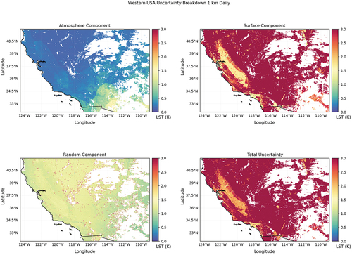
Figure A2. An uncertainty breakdown for Western U.S.A. region, at 1 km monthly for July 2021. Highlighting four key uncertainty components including atmosphere, surface, random and total uncertainty.

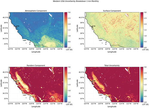
Greenland’s surface types are majorly homogenous ice and snow and dry atmosphere, resulting in the surface component dominating the 1 km daily total uncertainties (Figure A3). On a monthly scale (Figure A4), significant cloud cover and surface cover transitions from ice to bedrock around the coasts would contribute to the large sampling uncertainty, which propagates over time and increases total uncertainties.

Figure A3. An uncertainty breakdown for Greenland, at 1 km daily on 12/7/2021. Highlighting four key uncertainty components including atmosphere, surface, random and total uncertainty.

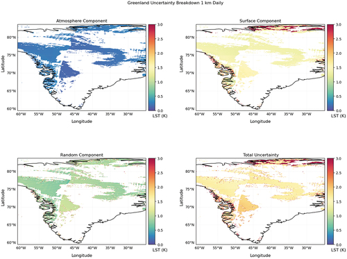
Figure A4. An uncertainty breakdown for Greenland, at 1 km monthly for July 2021. Highlighting four key uncertainty components including atmosphere, surface, random and total uncertainty.

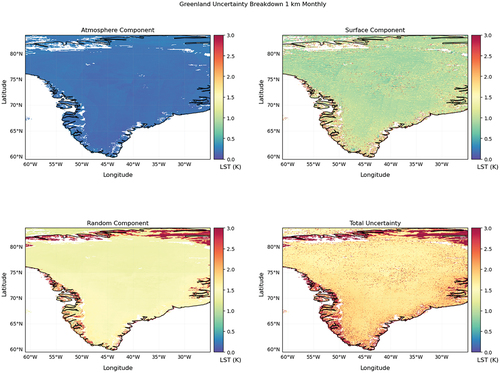
Europe’s surface and emissivity characteristics vary between countries and regions, which contributes to a large sampling uncertainty over the sampled region of interest. Water vapour from vegetation cover and contrasting rural and urban surface types appear to have a larger influence on the total uncertainty on a daily scale (Figure A5), especially towards southern France and Spain. However, Europe’s cloudy conditions and LST variance result in a random component dominance in total LST through uncertainty propagation on a monthly scale (Figure A6).

Figure A5. An uncertainty breakdown for Western Europe, at 1 km daily on 15/7/2021. Highlighting four key uncertainty components including atmosphere, surface, random and total uncertainty.

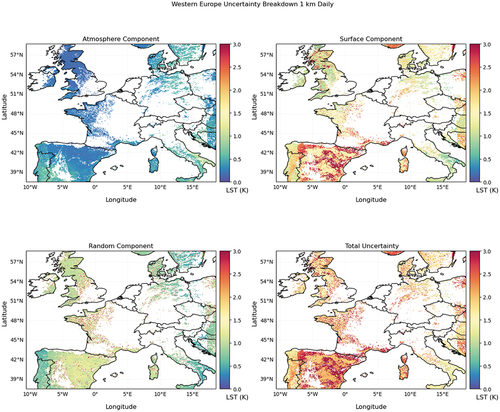
Figure A6. An uncertainty breakdown for Western Europe, at 1 km monthly for July 2021. Highlighting four key uncertainty components including atmosphere, surface, random and total uncertainty.

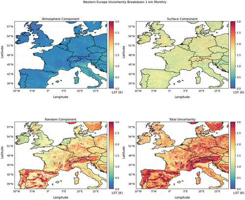
The sampled region of southeast China reflects a more even split of components in the total uncertainty on both a daily and monthly scale due to its relatively homogenous grasslands. Figure A7 highlights vegetative water vapour and surface characteristics that contribute to the total uncertainty. Figure A8 highlights the LST variance towards the north-western region of China, where surface cover transitions towards bare land. Furthermore, a larger atmosphere is dominant in the monthly total uncertainty from vegetation water vapour contribution in the south.

Figure A7. An uncertainty breakdown for China, at 1 km daily on 14/7/2021. Highlighting four key uncertainty components including atmosphere, surface, random and total uncertainty.

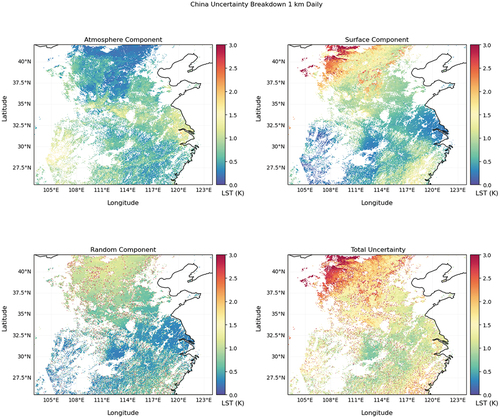
Figure A8. An uncertainty breakdown for China, at 1 km monthly for July 2021. Highlighting four key uncertainty components including atmosphere, surface, random and total uncertainty.

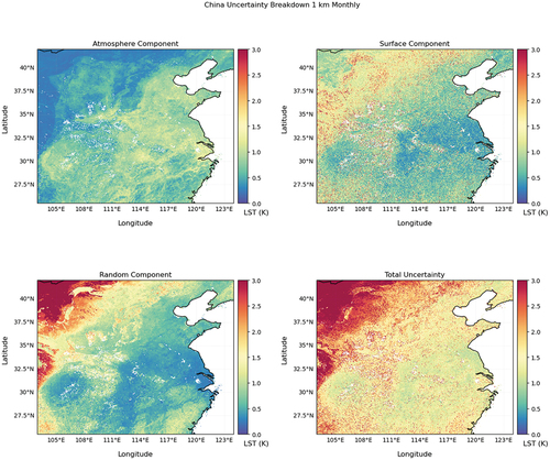
India’s atmosphere component clearly dominates the total uncertainty on a daily scale (Figure A9) from the seasonal effects of the summer monsoon in July. Propagation over time demonstrates that the atmosphere and random components drive the monthly total uncertainty (Figure A10) as a result of water vapour and large sampling uncertainties from cloud cover.

Figure A9. An uncertainty breakdown for India, at 1 km daily on 15/7/2021. Highlighting four key uncertainty components including atmosphere, surface, random and total uncertainty.

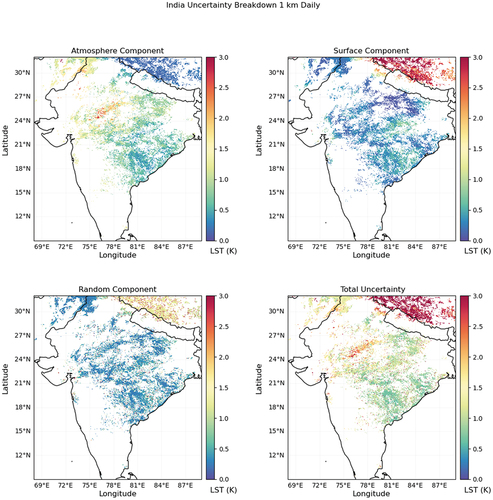
Figure A10. An uncertainty breakdown for India, at 1 km monthly for July 2021. Highlighting four key uncertainty components including atmosphere, surface, random and total uncertainty.

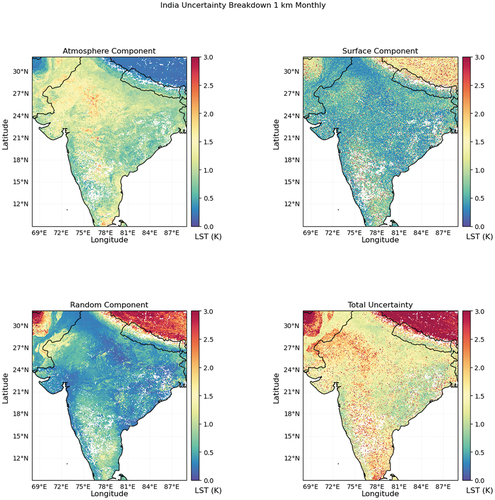
The Sahel region is a transition zone from the Saharan desert to the north and savannah to the south, which are clearly reflected within the daily total uncertainties (Figure A11). The monthly propagation (Figure A12) demonstrates how the random component dominates over the desert when propagated due to higher LST variance in the sampling uncertainty equation, reflected in the total uncertainty.

Figure A11. An uncertainty breakdown for the Sahel region, at 1 km daily on 9/7/2021. Highlighting four key uncertainty components including atmosphere, surface, random and total uncertainty.

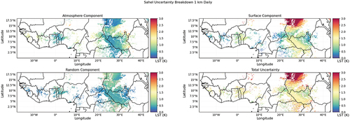
Figure A12. An uncertainty breakdown for the Sahel region, at 1 km monthly for July 2021. Highlighting four key uncertainty components including atmosphere, surface, random and total uncertainty.

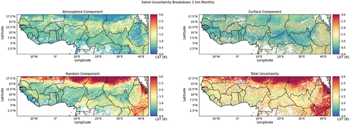
Siberia’s uncertainties on a daily scale (Figure A13) show how the total uncertainty is completely dominated by the surface component from various land cover types over a large region. This contributes to a large LST variance in the sampling uncertainty, propagated through the random component, which dominates on the monthly scale (Figure A14).

Figure A13. An uncertainty breakdown for Siberia, at 1 km daily on 15/7/2021. Highlighting four key uncertainty components including atmosphere, surface, random and total uncertainty.

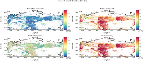
Figure A14. An uncertainty breakdown for Siberia, at 1 km monthly for July 2021. Highlighting four key uncertainty components including atmosphere, surface, random and total uncertainty.

References

- Arias, P. A., N. Bellouin, E., Coppola, R. Jones, G. Krinner, J., Marotzke, V. Naik, Palmer, M. D., Plattner, G. K., Rogelj, J., Rojas, M., et al. 2021. “I Technical Summary.“ In Climate Change 2021: The Physical Science Basis. Contribution of Working Group I to the Sixth Assessment Report of the Intergovernmental Panel on Climate Change, edited by Masson-Delmotte, V. P., Zhai, A., Pirani, S. L., Péan, C., Berger, S., Caud, N., Chen, Y., Goldfarb, M. I., Huang, M., Leitzell, K., Lonnoy, E., Matthews, J. B. R., Maycock, T. K., Waterfield, T., Yelekçi, O., Yu, R., and Zhou, B., 33−144. Cambridge, United Kingdom and New York, NY, USA: Cambridge University Press. https://doi.org/10.1017/9781009157896.002.
- Barnes, W. L., T. S. Pagano, and V. V. Salomonson. 1998. “Prelaunch Characteristics of the Moderate Resolution Imaging Spectroradiometer (Modis) on Eos-Am1.” IEEE Transactions on Geoscience and Remote Sensing 36 (4): 1088–1100. https://doi.org/10.1109/36.700993.
- Barrett, B. S., G. R. Henderson, E. McDonnell, M. Henry, and T. Mote. 2020. “Extreme Greenland Blocking and High-Latitude Moisture Transport.” Atmospheric Science Letters 21 (11): e1002. https://doi.org/10.1002/asl.1002.
- Basha, G., P. Kishore, M. V. Ratnam, A. Jayaraman, A. Agha Kouchak, T. B. Ouarda, and I. Velicogna. 2017. “Historical and Projected Surface Temperature Over India During the 20th and 21st Century.” Scientific Reports 7 (1): 2987. https://doi.org/10.1038/s41598-017-02130-3.
- Batbaatar, J., A. R. Gillespie, R. S. Sletten, A. Mushkin, R. Amit, D. Trombotto Liaudat, L. Liu, and G. Petrie. 2020. “Toward the Detection of Permafrost Using Land-Surface Temperature Mapping.” Remote Sensing 12 (4): 695. https://doi.org/10.3390/rs12040695.
- Becker, F., and Z.-L. Li. 1990. “Towards a Local Split Window Method Over Land Surfaces.” International Journal of Remote Sensing 11 (3): 369–393. https://doi.org/10.1080/01431169008955028.
- Belward, A., M. Bourassa, M. Dowell, S. Briggs, H. Dolman, K. Holmlund, and M. Verstraete. 2016. The global observing system for climate: Implementation needs. GCOS-200.
- Bento, V. A., C. M. Gouveia, C. C. DaCamara, R. Libonati, and I. F. Trigo. 2020. “The Roles of NDVI and Land Surface Temperature When Using the Vegetation Health Index Over Dry Regions.” Global and Planetary Change 190:103198. https://doi.org/10.1016/j.gloplacha.2020.103198.
- Biasutti, M. 2019. “Rainfall Trends in the African Sahel: Characteristics, Processes, and Causes.” Wires Clim Change 10 (4): e591. https://doi.org/10.1002/wcc.591.
- Box, M. A., and G. P. Box. 2016. Physics of Radiation and Climate. CRC Press, Taylor and Francis Group. https://doi.org/10.1201/b19395.
- Carvalho, D., S. Cardoso Pereira, and A. Rocha. 2021. “Future Surface Temperatures Over Europe According to Cmip6 Climate Projections: An Analysis with Original and Bias-Corrected Data.” Climatic Change 167 (1): 1–17. https://doi.org/10.1007/s10584-021-03159-0.
- Chen, Y., K. Yang, J. He, J. Qin, J. Shi, J. Du, and Q. He. 2011. “Improving Land Surface Temperature Modeling for Dry Land of China.” Journal of Geophysical Research Atmospheres 116 (D20). https://doi.org/10.1029/2011JD015921.
- Coolidge, F. L. 2020. Statistics: A Gentle Introduction. California: Sage Publications.
- Cox, D. T., I. M. Maclean, A. S. Gardner, and K. J. Gaston. 2020. “Global Variation in Diurnal Asymmetry in Temperature, Cloud Cover, Specific Humidity and Precipitation and Its Association with Leaf Area Index.” Global Change Biology 26 (12): 7099–7111. https://doi.org/10.1111/gcb.15336.
- Davini, P., C. Cagnazzo, R. Neale, and J. Tribbia. 2012. “Coupling Between Greenland Blocking and the North Atlantic Oscillation Pattern.” Geophysical Research Letters 39 (14). https://doi.org/10.1029/2012GL052315.
- De Kauwe, M. G., C. M. Taylor, P. P. Harris, G. P. Weedon, and R. J. Ellis. 2013. “Quantifying Land Surface Temperature Variability for Two Sahelian Mesoscale Regions During the Wet Season.” Journal of Hydrometeorology 14 (5): 1605–1619. https://doi.org/10.1175/JHM-D-12-0141.1.
- Deshpande, N., A. Kulkarni, and K. Krishna Kumar. 2012. “Characteristic Features of Hourly Rainfall in India.” International Journal of Climatology 32 (11): 1730–1744. https://doi.org/10.1002/joc.2375.
- Doyle, S. H., A. Hubbard, A. A. Fitzpatrick, D. van as, A. B. Mikkelsen, R. Pettersson, and B. Hubbard. 2014. “Persistent Flow Acceleration within the Interior of the Greenland Ice Sheet.” Geophysical Research Letters 41 (3): 899–905. https://doi.org/10.1002/2013GL058933.
- Draper, N. R., and H. Smith. 1998. Applied Regression Analysis. Vol. 326. John Wiley & Sons. https://doi.org/10.1002/9781118625590.
- Duan, P., and S. Li. 2019. “Relationship between land surface temperature and land use/land cover in Taiyuan, China . In Fifth Symposium on Novel Optoelectronic Detection Technology and Application. Vol. 11023. 619–630. SPIE. https://doi.org/10.1117/12.2521120March.
- Duan, S.-B., Z.-L. Li, and P. Leng. 2017. “A Framework for the Retrieval of All-Weather Land Surface Temperature at a High Spatial Resolution from Polar-Orbiting Thermal Infrared and Passive Microwave Data.” Remote Sensing of Environment 195:107–117. https://doi.org/10.1016/j.rse.2017.04.008.
- Durbin, J., and G. Watson. 1950. “Testing for Serial Correlation in Least Squares Regression.” In i biometrika, 409–428. Vol. 37 (Oxford: Oxford University Press, Biometrika Trust).
- Durbin, J., and G. Watson. 1951. “Testing for Serial Correlation in Least Squares Regression.” ii Biometrika 38 (1/2): 159–178.
- Epule, E. T., C. Peng, L. Lepage, and Z. Chen. 2014. “The Causes, Effects and Challenges of Sahelian Droughts: A Critical Review.” Regional Environmental Change 14 (1): 145–156. https://doi.org/10.1007/s10113-013-0473-z.
- ESA. 2019. Land Surface Temperature CCI Algorithm Theoretical Basis Document. Report. LST-CCI-D2.2-ATBD.
- ESA. 2021. European space agency, land surface temperature-cci-product user guide. wp4a– del-d4.3.
- Evans, J. P., and I. Boyer-Souchet. 2012. “Local Sea Surface Temperatures Add to Extreme Precipitation in Northeast Australia During la Niña.” Geophysical Research Letters 39 (10). https://doi.org/10.1029/2012GL052014.
- Freitas, S. C., I. F. Trigo, J. M. Bioucas-Dias, and F. M. Gottsche. 2010. “Quantifying the Uncertainty of Land Surface Temperature Retrievals from Seviri/Meteosat.” IEEE Transactions on Geoscience and Remote Sensing 48 (1): 523–534. https://doi.org/10.1109/TGRS.2009.2027697.
- Fu, P., and Q. Weng. 2016. “A Time Series Analysis of Urbanization Induced Land Use and Land Cover Change and Its Impact on Land Surface Temperature with Landsat Imagery.” Remote Sensing of Environment 175:205–214. https://doi.org/10.1016/j.rse.2015.12.040.
- Ganter, C. 2011. “Seasonal Climate Summary Southern Hemisphere (Winter 2010): A Fast Developing la Niña.” Australian Meteorological and Oceanographic Journal 61 (2): 125. https://doi.org/10.22499/2.6102.005.
- García-Herrera, R., J. Díaz, R. M. Trigo, J. Luterbacher, and E. M. Fischer. 2010. “A Review of the European Summer Heat Wave of 2003.” Critical Reviews in Environmental Science and Technology 40 (4): 267–306. https://doi.org/10.1080/10643380802238137.
- Gautam, R., N. Hsu, K.-M. Lau, and M. Kafatos. 2009. “Aerosol and Rainfall Variability Over the Indian Monsoon Region: Distributions, Trends and Coupling.” In Annales Geophysicae, 3691–3703. Vol. 27, Germany: Copernicus GmbH.
- Geng, X., D. Zhang, C. Li, Y. Yuan, Z. Yu, and X. Wang. 2022. “Impacts of Climatic Zones on Urban Heat Island: Spatiotemporal Variations, Trends, and Drivers in China from 2001–2020.” Sustainable Cities and Society 89:104303. https://doi.org/10.1016/j.scs.2022.104303.
- Ghent, D., G. Corlett, F.-M. Göttsche, and J. Remedios. 2017. “Global Land Surface Temperature from the Along-Track Scanning Radiometers.” Journal of Geophysical Research: Atmospheres 122 (22): 12–167. https://doi.org/10.1002/2017JD027161.
- Ghent, D., K. Veal, T. Trent, E. Dodd, H. Sembhi, and J. Remedios. 2019. “A New Approach to Defining Uncertainties for Modis Land Surface Temperature.” Remote Sensing 11 (9): 1021. https://doi.org/10.3390/rs11091021.
- Good, E., F. M. Aldred, D. J. Ghent, K. L. Veal, and C. Jimenez. 2022. “An Analysis of the Stability and Trends in the Lstcci Land Surface Temperature Datasets Over Europe.” Earth & Space Science 9 (9). https://doi.org/10.1029/2022EA002317.
- Good, E., D. J. Ghent, C. E. Bulgin, and J. J. Remedios. 2017. “A Spatiotemporal Analysis of the Relationship Between Near-Surface Air Temperature and Satellite Land Surface Temperatures Using 17 Years of Data from the Atsr Series.” Journal of Geophysical Research: Atmospheres 122 (17): 9185–9210. https://doi.org/10.1002/2017JD026880.
- Gouveia, C. M., J. P. Martins, A. Russo, R. Durão, and I. F. Trigo. 2022. “Monitoring Heat Extremes Across Central Europe Using Land Surface Temperature Data Records from Seviri/Msg.” Remote Sensing 14 (14): 3470. https://doi.org/10.3390/rs14143470.
- Gudmundsson, L., and S. I. Seneviratne. 2016. “Anthropogenic Climate Change Affects Meteorological Drought Risk in Europe.” Environmental Research Letters 11 (4): 044005. https://doi.org/10.1088/1748-9326/11/4/044005.
- Hall, D. K., R. Williams Jr, K. A. Casey, N. E. DiGirolamo, and Z. Wan. 2006. “Satellite-Derived, Melt-Season Surface Temperature of the Greenland Ice Sheet (2000–2005) and Its Relationship to Mass Balance.” Geophysical Research Letters 33 (11). https://doi.org/10.1029/2006GL026444.
- Hanna, E., T. E. Cropper, R. J. Hall, and J. Cappelen. 2016. “Greenland Blocking Index 1851–2015: A Regional Climate Change Signal.” International Journal of Climatology 36 (15): 4847–4861. https://doi.org/10.1002/joc.4673.
- Heidemann, H., J. Ribbe, T. Cowan, B. J. Henley, C. Pudmenzky, R. Stone, and D. H. Cobon. 2022. “The Influence of Interannual and Decadal Indo-Pacific Sea Surface Temperature Variability on Australian Monsoon Rainfall.” Journal of Climate 35 (1): 425–444.
- Hellings, A., and A. Rienow. 2021. “Mapping Land Surface Temperature Developments in Functional Urban Areas Across Europe.” Remote Sensing 13 (11): 2111. https://doi.org/10.3390/rs13112111.
- Hinzman, L. D., N. D. Bettez, W. R. Bolton, F. S. Chapin, M. B. Dyurgerov, C. L. Fastie, B. Griffith, R. D. Hollister, A. Hope, H. P. Huntington. 2005. “Evidence and Implications of Recent Climate Change in Northern Alaska and Other Arctic Regions.” Climatic Change 72 (3): 251–298. https://doi.org/10.1007/s10584-005-5352-2.
- Hinzman, L. D., C. J. Deal, A. D. McGuire, S. H. Mernild, I. V. Polyakov, and J. E. Walsh. 2013. “Trajectory of the Arctic as an Integrated System.” Ecological Applications 23 (8): 1837–1868. https://doi.org/10.1890/11-1498.1.
- Hofer, S., A. J. Tedstone, X. Fettweis, and J. L. Bamber. 2019. “Cloud Microphysics and Circulation Anomalies Control Differences in Future Greenland Melt.” Nature Climate Change 9 (7): 523–528. https://doi.org/10.1038/s41558-019-0507-8.
- Hook, S. 2017. Combined ASTER and MODIS Emissivity Database Over Land (CAMEL) Emissivity Monthly Global 0.05deg V002. https://doi.org/10.5067/MEaSUREs/LSTE/CAM5K30EM.002.
- Hulley, G., and D. Ghent. 2019. Taking the Temperature of the Earth: steps towards integrated understanding of variability and change. Netherlands: Elsevier.
- Hulley, G. C., and S. J. Hook. 2012. “A Radiance-Based Method for Estimating Uncertainties in the Atmospheric Infrared Sounder (Airs) Land Surface Temperature Product.” Journal of Geophysical Research: Atmospheres 117 (D20). https://doi.org/10.1029/2012JD018102.
- Hunt, K. M., and J. K. Fletcher. 2019. “The Relationship Between Indian Monsoon Rainfall and Low-Pressure Systems.” Climate Dynamics 53 (3): 1859–1871. https://doi.org/10.1007/s00382-019-04744-x.
- Hurrell, J. W. 1995. “Decadal Trends in the North Atlantic Oscillation: Regional Temperatures and Precipitation.” Science: Advanced Materials and Devices 269 (5224): 676–679. https://doi.org/10.1126/science.269.5224.676.
- Ives, A. R., L. Zhu, F. Wang, J. Zhu, C. J. Morrow, and V. C. Radeloff. 2021. “Statistical Inference for Trends in Spatiotemporal Data.” Remote Sensing of Environment 266:112678. https://doi.org/10.1016/j.rse.2021.112678.
- Jia, X., P. Song, G. Yun, A. Li, K. Wang, K. Zhang, C. Du, Y. Feng, K. Qu, M. Wu. 2022. “Effect of Landscape Structure on Land Surface Temperature in Different Essential Urban Land Use Categories: A Case Study in Jiaozuo, China.” Land 11 (10): 1687. https://doi.org/10.3390/land11101687.
- Jiménez-Muñoz, J. C., J. A. Sobrino, C. Mattar, and Y. Malhi. 2013. “Spatial and Temporal Patterns of the Recent Warming of the Amazon Forest.” Journal of Geophysical Research: Atmospheres 118 (11): 5204–5215. https://doi.org/10.1002/jgrd.50456.
- Jin, Q., and C. Wang. 2017. “A Revival of Indian Summer Monsoon Rainfall Since 2002.” Nature Climate Change 7 (8): 587–594. https://doi.org/10.1038/nclimate3348.
- Joint Committee for Guides in Metrology. 2008. Evaluation of Measurement Data—Guide to the Expression of Uncertainty in Measurement. Bureau International des Poids et Mesures.
- Jones, P., and D. Lister. 2009. “The Influence of the Circulation on Surface Temperature and Precipitation Patterns Over Europe.” Climate of the Past 5 (2): 259–267. https://doi.org/10.5194/cp-5-259-2009.
- Katzenberger, A., J. Schewe, J. Pongratz, and A. Levermann. 2021. “Robust Increase of Indian Monsoon Rainfall and Its Variability Under Future Warming in Cmip6 Models.” Earth System Dynamics 12 (2): 367–386. https://doi.org/10.5194/esd-12-367-2021.
- Kjellström, E., P. Thejll, M. Rummukainen, J. H. Christensen, F. Boberg, O. B. Christensen, and C. F. Maule. 2013. “Emerging Regional Climate Change Signals for Europe Under Varying Large-Scale Circulation Conditions.” Climate Research 56 (2): 103–119. https://doi.org/10.3354/cr01146.
- Kogan, F., and W. Guo. 2015. “2006–2015 Mega-Drought in the Western USA and Its Monitoring from Space Data.” Geomatics, Natural Hazards and Risk 6 (8): 651–668. https://doi.org/10.1080/19475705.2015.1079265.
- Krämer, W. 2011. “Durbin–watson test.” In International Encyclopedia of Statistical Science, 408–409. Springer Berlin Heidelberg. https://doi.org/10.1007/978-3-642-04898-2_219.
- Krishnan, R., and V. Ramanathan. 2002. “Evidence of Surface Cooling from Absorbing Aerosols.” Geophysical Research Letters 29 (9): 54–1. https://doi.org/10.1029/2002GL014687.
- Langer, M., S. Westermann, S. Muster, K. Piel, and J. Boike. 2011. “The Surface Energy Balance of a Polygonal Tundra Site in Northern Siberia–Part 1: Spring to Fall.” The Cryosphere 5 (1): 151–171. https://doi.org/10.5194/tc-5-151-2011.
- Lawrence, D., and K. Vandecar. 2015. “Effects of Tropical Deforestation on Climate and Agriculture.” Nature Climate Change 5 (1): 27–36. https://doi.org/10.1038/nclimate2430.
- Leeper, R. D., R. Bilotta, B. Petersen, C. J. Stiles, R. Heim, B. Fuchs, O. P. Prat, M. Palecki, and S. Ansari. 2022. “Characterizing U.S. Drought Over the Past 20 years Using the U.S. Drought Monitor.” International Journal of Climatology 42 (12): 6616–6630. https://doi.org/10.1002/joc.7653.
- Lejeune, Q., E. L. Davin, B. P. Guillod, and S. I. Seneviratne. 2015. “Influence of Amazonian Deforestation on the Future Evolution of Regional Surface Fluxes, Circulation, Surface Temperature and Precipitation.” Climate Dynamics 44 (9): 2769–2786. https://doi.org/10.1007/s00382-014-2203-8.
- Li, J., Z.-L. Li, H. Wu, and N. You. 2022. “Trend, Seasonality, and Abrupt Change Detection Method for Land Surface Temperature Time-Series Analysis: Evaluation and Improvement.” Remote Sensing of Environment 280:113222. https://doi.org/10.1016/j.rse.2022.113222.
- Liu, Z., A. P. Ballantyne, and L. A. Cooper. 2018. “Increases in Land Surface Temperature in Response to Fire in Siberian Boreal Forests and Their Attribution to Biophysical Processes.” Geophysical Research Letters 45 (13): 6485–6494. https://doi.org/10.1029/2018GL078283.
- Liu, Y., X. Fang, Y. Xu, S. Zhang, and Q. Luan. 2018. “Assessment of Surface Urban Heat Island Across China’s Three Main Urban Agglomerations.” Theoretical and Applied Climatology 133 (1): 473–488. https://doi.org/10.1007/s00704-017-2197-3.
- Liu, J., D. F. T. Hagan, and Y. Liu. 2020. “Global Land Surface Temperature Change (2003–2017) and Its Relationship with Climate Drivers: Airs, Modis, and Era5-Land Based Analysis.” Remote Sensing 13 (1): 44. https://doi.org/10.3390/rs13010044.
- Li, Z.-L., H. Wu, S.-B. Duan, W. Zhao, H. Ren, X. Liu, P. Leng, R. Tang, X. Ye, J. Zhu, et al. 2023. “Satellite Remote Sensing of Global Land Surface Temperature: Definition, Methods, Products, and Applications.” Reviews of Geophysics 61 (1): e2022RG000777. https://doi.org/10.1029/2022RG000777.
- Lu, C. 2017. “A Modified Algorithm for Identifying and Tracking Extratropical Cyclones.” Advances in Atmospheric Sciences 34 (7): 909–924. https://doi.org/10.1007/s00376-017-6231-2.
- Lu, J. 2009. “The Dynamics of the Indian Ocean Sea Surface Temperature Forcing of Sahel Drought.” Climate Dynamics 33 (4): 445–460. https://doi.org/10.1007/s00382-009-0596-6.
- Luterbacher, J., D. Dietrich, E. Xoplaki, M. Grosjean, and H. Wanner. 2004. “European Seasonal and Annual Temperature Variability, Trends, and Extremes Since 1500.” Science: Advanced Materials and Devices 303 (5663): 1499–1503. https://doi.org/10.1126/science.1093877.
- Lu, C., Y. Zhang, and Z. Guan. 2022. “Winter Anticyclone Activities in Siberia and Their Relationship to the Regional Temperature Anomaly.” International Journal of Climatology 42 (12): 6293–6310. https://doi.org/10.1002/joc.7590.
- Mantua, N. J., and S. R. Hare. 2002. “The Pacific Decadal Oscillation.” Journal of Oceanography 58 (1): 35–44. https://doi.org/10.1023/A:1015820616384.
- Merchant, C. J., F. Paul, T. Popp, M. Ablain, S. Bontemps, P. Defourny, R. Hollmann, et al. 2017. “Uncertainty Information in Climate Data Records from Earth Observation.” Earth System Science Data 9 (2): 511–527. https://doi.org/10.5194/essd-9-511-2017.
- MetOffice. 2019. “The Heatwave of 2003.” Online; Accessed November 21, 2022. https://www.metoffice.gov.uk/weather/learn-about/weather/case-studies/heatwave.
- Muro, J., A. Strauch, S. Heinemann, S. Steinbach, F. Thonfeld, B. Waske, and B. Diekkrüger. 2018. “Land Surface Temperature Trends as Indicator of Land Use Changes in Wetlands.” International Journal of Applied Earth Observation and Geoinformation 70:62–71. https://doi.org/10.1016/j.jag.2018.02.002.
- Muster, S., M. Langer, A. Abnizova, K. L. Young, and J. Boike. 2015. “Spatio-Temporal Sensitivity of Modis Land Surface Temperature Anomalies Indicates High Potential for Large-Scale Land Cover Change Detection in Arctic Permafrost Landscapes.” Remote Sensing of Environment 168:1–12. https://doi.org/10.1016/j.rse.2015.06.017.
- Newey, W. K., and K. D. West. 1987. “Hypothesis Testing with Efficient Method of Moments Estimation.” International Economic Review 28 (3): 777–787. https://doi.org/10.2307/2526578.
- Nick, F., A. Luckman, A. Vieli, C. J. Van der Veen, D. Van as, R. Van De Wal, F. Pattyn, A. Hubbard, and D. Floricioiu. 2012. “The Response of Petermann Glacier, Greenland, to Large Calving Events, and Its Future Stability in the Context of Atmospheric and Oceanic Warming.” Journal of Glaciology 58 (208): 229–239. https://doi.org/10.3189/2012JoG11J242.
- Norman, J. M., and F. Becker. 1995. “Terminology in the Thermal Infrared Remote Sensing of Natural Surfaces.” Agricultural and Forest Meteorology 77 77 (3–4): 153–166. https://doi.org/10.1016/0168-1923(95)02259-Z.
- Popp, T., M. I. Hegglin, R. Hollmann, F. Ardhuin, A. Bartsch, A. Bastos, V. Bennett, et al. 2020. “Consistency of Satellite Climate Data Records for Earth System Monitoring.” Bulletin of the American Meteorological Society 101 (11): E1948–E1971. https://doi.org/10.1175/BAMS-D-19-0127.1.
- Ratna, S. B., A. Cherchi, T. J. Osborn, M. Joshi, and U. Uppara. 2021. “The Extreme Positive Indian Ocean Dipole of 2019 and Associated Indian Summer Monsoon Rainfall Response.” Geophysical Research Letters 48 (2): e2020GL091497. https://doi.org/10.1029/2020GL091497.
- Retamales-Muñoz, G., C. Durán-Alarcón, and C. Mattar. 2019. “Recent Land Surface Temperature Patterns in Antarctica Using Satellite and Reanalysis Data.” Journal of South American Earth Sciences 95:102304. https://doi.org/10.1016/j.jsames.2019.102304.
- Rippey, B. R. 2015. “The Us Drought of 2012.” Weather and Climate Extremes 10:57–64. https://doi.org/10.1016/j.wace.2015.10.004.
- Risbey, J. S., M. J. Pook, P. C. McIntosh, M. C. Wheeler, and H. H. Hendon. 2009. “On the Remote Drivers of Rainfall Variability in Australia.” Monthly Weather Review 137 (10): 3233–3253. https://doi.org/10.1175/2009MWR2861.1.
- Rodríguez-Fonseca, B., E. Mohino, C. R. Mechoso, C. Caminade, M. Biasutti, M. Gaetani, J. García-Serrano, et al. 2015. “Variability and Predictability of West African Droughts: A Review on the Role of Sea Surface Temperature Anomalies.” Journal of Climate 28 (10): 4034–4060. https://doi.org/10.1175/JCLI-D-14-00130.1.
- Ross, R. S., T. Krishnamurti, S. Pattnaik, and D. Pai. 2018. “Decadal Surface Temperature Trends in India Based on a New High-Resolution Data Set.” Scientific Reports 8 (1): 1–10. https://doi.org/10.1038/s41598-018-25347-2.
- Roth, M. 2012. Urban Heat Islands. In Handbook of Environmental Fluid Dynamics, edited by H.J.S. Fernando. Boca Raton: CRC Press, Routledge Handbooks Online CRC Press 12 Dec 2012 accessed 21 Sep 2022.
- Röthlisberger, M., L. Frossard, L. F. Bosart, D. Keyser, and O. Martius. 2019. “Recurrent Synoptic-Scale Rossby Wave Patterns and Their Effect on the Persistence of Cold and Hot Spells.” Journal of Climate 32 (11): 3207–3226. https://doi.org/10.1175/JCLI-D-18-0664.1.
- Saint-Lu, M., R. Chadwick, F. H. Lambert, and M. Collins. 2019. “Surface Warming and Atmospheric Circulation Dominate Rainfall Changes Over Tropical Rainforests Under Global Warming.” Geophysical Research Letters 46 (22): 13410–13419. https://doi.org/10.1029/2019GL085295.
- Serreze, M., J. Walsh, F. Chapin, T. Osterkamp, M. Dyurgerov, V. Romanovsky, W. Oechel, J. Morison, T. Zhang, and R. Barry. 2000. “Observational Evidence of Recent Change in the Northern High-Latitude Environment.” Climatic Change 46 (1): 159–207. https://doi.org/10.1023/A:1005504031923.
- Sobrino, J. A., J. C. Jiménez-Muñoz, G. Sòria, M. Romaguera, L. Guanter, J. Moreno, A. Plaza, and P. Martínez. 2008. “Land Surface Emissivity Retrieval from Different Vnir and Tir Sensors.” IEEE Transactions on Geoscience and Remote Sensing 46 (2): 316–327. https://doi.org/10.1109/TGRS.2007.904834.
- Sobrino, J. A., Y. Julien, and S. García-Monteiro. 2020. “Surface Temperature of the Planet Earth from Satellite Data.” Remote Sensing 12 (2): 218. https://doi.org/10.3390/rs12020218.
- Song, Z., R. Li, R. Qiu, S. Liu, C. Tan, Q. Li, W. Ge, et al. 2018. “Global Land Surface Temperature Influenced by Vegetation Cover and Pm2. 5 from 2001 to 2016.” Remote Sensing 10 (12): 2034. https://doi.org/10.3390/rs10122034.
- Song, Z., H. Yang, X. Huang, W. Yu, J. Huang, and M. Ma. 2021. “The Spatiotemporal Pattern and Influencing Factors of Land Surface Temperature Change in China from 2003 to 2019.” International Journal of Applied Earth Observation and Geoinformation 104:102537. https://doi.org/10.1016/j.jag.2021.102537.
- Spies, R. B. 2006. Long-Term Ecological Change in the Northern Gulf of Alaska. Netherlands: Elsevier.
- Steinke, S., S. Eikenberg, U. Löhnert, G. Dick, D. Klocke, P. Di Girolamo, and S. Crewell. 2015. “Assessment of Small-Scale Integrated Water Vapour Variability During Hope.” Atmospheric Chemistry and Physics 15 (5): 2675–2692. https://doi.org/10.5194/acp-15-2675-2015.
- Stephens, L. J. 2018. Schaum’s Outline of Statistics. Maidenhead, UK: McGraw-Hill Education.
- Swann, A. L., M. Longo, R. G. Knox, E. Lee, and P. R. Moorcroft. 2015. “Future Deforestation in the Amazon and Consequences for South American Climate.” Agricultural and Forest Meteorology 214:12–24. https://doi.org/10.1016/j.agrformet.2015.07.006.
- Tomlinson, C. J., L. Chapman, J. E. Thornes, and C. Baker. 2011. “Remote Sensing Land Surface Temperature for Meteorology and Climatology: A Review.” Meteorological Applications 18 (3): 296–306. https://doi.org/10.1002/met.287.
- Turner, P. 2020. “Critical Values for the Durbin-Watson Test in Large Samples.” Applied Economics Letters 27 (18): 1495–1499. https://doi.org/10.1080/13504851.2019.1691711.
- Van as, D., A. Hubbard, B. Hasholt, A. Mikkelsen, M. Van den Broeke, and R. Fausto. 2012. “Large Surface Meltwater Discharge from the Kangerlussuaq Sector of the Greenland Ice Sheet During the Record-Warm Year 2010 Explained by Detailed Energy Balance Observations.” The Cryosphere 6 (1): 199–209. https://doi.org/10.5194/tc-6-199-2012.
- Vecchio, A. L., M. Lenzano, M. Durand, E. Lannutti, R. Bruce, and L. Lenzano. 2018. “Estimation of Surface Flow Speed and Ice Surface Temperature from Optical Satellite Imagery at Viedma Glacier, Argentina.” Global and Planetary Change 169:202–213. https://doi.org/10.1016/j.gloplacha.2018.08.001.
- Wan, Z. 2002. “Estimate of Noise and Systematic Error in Early Thermal Infrared Data of the Moderate Resolution Imaging Spectroradiometer (Modis).” Remote Sensing of Environment 80 (1): 47–54. https://doi.org/10.1016/S0034-4257(01)00266-8.
- Wan, Z., and J. Dozier. 1996. “A Generalized Split-Window Algorithm for Retrieving Land-Surface Temperature from Space.” IEEE Transactions on Geoscience and Remote Sensing 34 (4): 892–905. https://doi.org/10.1109/36.508406.
- Wang, P., Q. Huang, Q. Tang, X. Chen, J. Yu, S. P. Pozdniakov, and T. Wang. 2021. “Increasing Annual and Extreme Precipitation in Permafrost-Dominated Siberia During 1959–2018.” Journal of Hydrology 603:126865. https://doi.org/10.1016/j.jhydrol.2021.126865.
- Wan, Z., P. Wang, and X. Li. 2010. “Using Modis Land Surface Temperature and Normalized Difference Vegetation Index Products for Monitoring Drought in the Southern Great Plains, Usa.” International Journal of Remote Sensing 25 (1): 61–72. https://doi.org/10.1080/0143116031000115328.
- Wardle, R., and I. Smith. 2004. “Modeled Response of the Australian Monsoon to Changes in Land Surface Temperatures.” Geophysical Research Letters 31 (16). https://doi.org/10.1029/2004GL020157.
- Weatherhead, E. C., G. C. Reinsel, G. C. Tiao, X.-L. Meng, D. Choi, W.-K. Cheang, T. Keller, et al. 1998. “Factors Affecting the Detection of Trends: Statistical Considerations and Applications to Environmental Data.” Journal of Geophysical Research Atmospheres 103 (D14): 17149–17161. https://doi.org/10.1029/98JD00995.
- Weatherhead, E. C., A. J. Stevermer, and B. E. Schwartz. 2002. “Detecting Environmental Changes and Trends.” Physics and Chemistry of the Earth, Parts A/B/C 27 (6–8): 399–403. https://doi.org/10.1016/S1474-7065(02)00019-0.
- Weng, Q. 2009. “Thermal Infrared Remote Sensing for Urban Climate and Environmental Studies: Methods, Applications, and Trends.” ISPRS Journal of Photogrammetry and Remote Sensing 64 (4): 335–344. https://doi.org/10.1016/j.isprsjprs.2009.03.007.
- Westergaard-Nielsen, A., M. Karami, B. Hansen, S. Westermann, and B. Elberling. 2018. “Contrasting Temperature Trends Across the Ice-Free Part of Greenland.” Scientific Reports 8 (1): 1586. https://doi.org/10.1038/s41598-018-19992-w.
- Wheeler, M. C., H. H. Hendon, S. Cleland, H. Meinke, and A. Donald. 2009. “Impacts of the Madden–Julian Oscillation on Australian Rainfall and Circulation.” Journal of Climate 22 (6): 1482–1498. https://doi.org/10.1175/2008JCLI2595.1.
- Whitley, E., and J. Ball. 2002. “Statistics Review 3: Hypothesis Testing and P Values.” Critical Care 6 (1): 3–4. https://doi.org/10.1186/cc1442.
- Wyss, D., K. Negussie, A. Staacke, A. Karnagel, M. Engelhardt, and M. Kappas. 2022. “A Comparative Analysis of Modis-Derived Drought Indices for Northern and Central Namibia.” African Journal of Environmental Science and Technology 16 (5): 173–191. https://doi.org/10.5897/AJEST2022.3096.
- Xiao, R., Q. Weng, Z. Ouyang, W. Li, E. W. Schienke, and Z. Zhang. 2008. “Land Surface Temperature Variation and Major Factors in Beijing, China.” Photogrammetric Engineering & Remote Sensing 74 (4): 451–461. https://doi.org/10.14358/PERS.74.4.451.
- Yan, Y., K. Mao, J. Shi, S. Piao, X. Shen, J. Dozier, Y. Liu, H.-L. Ren, and Q. Bao. 2020. “Driving Forces of Land Surface Temperature Anomalous Changes in North America in 2002– 2018.” Scientific Reports 10 (1): 1–13. https://doi.org/10.1038/s41598-020-63701-5.
- Yoo, S.-H., J. Fasullo, S. Yang, and C.-H. Ho. 2010. “On the Relationship Between Indian Ocean Sea Surface Temperature and the Transition from el Niño to la Niña.” Journal of Geophysical Research: Atmospheres 115 (D15). https://doi.org/10.1029/2009JD012978.
- Yoshikawa, K., and L. D. Hinzman. 2003. “Shrinking Thermokarst Ponds and Groundwater Dynamics in Discontinuous Permafrost Near Council, Alaska.” Permafrost and Periglacial Processes 14 (2): 151–160. https://doi.org/10.1002/ppp.451.
- Yoshioka, M., N. M. Mahowald, A. J. Conley, W. D. Collins, D. W. Fillmore, C. S. Zender, and D. B. Coleman. 2007. “Impact of Desert Dust Radiative Forcing on Sahel Precipitation: Relative Importance of Dust Compared to Sea Surface Temperature Variations, Vegetation Changes, and Greenhouse Gas Warming.” Journal of Climate 20 (8): 1445–1467. https://doi.org/10.1175/JCLI4056.1.
- Yu, Y., and M. Notaro. 2020. “Observed Land Surface Feedbacks on the Australian Monsoon System.” Climate Dynamics 54 (5): 3021–3040. https://doi.org/10.1007/s00382-020-05154-0.