Comparing field measurements and annotations as training data for UAV-based detection of standing dead trees in coniferous forest

ABSTRACT

Deadwood provides a habitat for a large number of species and acts as a significant carbon storage. Thus, deadwood mapping allows planning various actions related to biodiversity conservation and forest management. Airborne laser scanning (ALS) provides an efficient means for monitoring large forested areas and is thus a potential method for deadwood mapping. Machine learning (ML) can be used for automating deadwood detection from ALS data. However, ML requires training data, collecting of which is laborious using field measurements. This study inspected the feasibility of training data manually annotated from aerial images for the mapping of individual standing dead trees. The standing dead trees were mapped from an ALS dataset collected with an unmanned aerial vehicle (UAV). The study was carried out by performing ML-based standing dead tree detection using annotated training data and field-measured training data, and comparing the performances of the models trained on these two datasets. The study found that using annotated training data improves the performance of standing dead tree detection due to its higher availability compared to field-measured data. For large trees (height > 14 m), the precision, recall, Cohen’s kappa score, and Matthews correlation coefficient achieved by the best classifier trained on annotated data were 0.23, 0.48, 0.17, and 0.20, respectively. In comparison, the corresponding metrics for the best classifier trained on field-measured data were 0.14, 0.52, 0.04, and 0.13. Annotated standing dead tree data is not a representative sample of the true standing dead tree population, as small trees and trees without crowns (snags) can often not be identified from aerial images. However, the study found that identifying such trees is challenging even when using field-measured training data, and thus using annotated training data does not bias results. In general, the results of the study showed that ALS-based standing dead tree detection should focus on the detection of large trees.

1. Introduction

Deadwood is an important element in the forest environment. A wide variety of species rely on it, including beetles, fungi, trees, and woodpeckers (Lassauce et al. 2011; Martinuzzi et al. 2009; Stokland, Siitonen, and Gunnar Jonsson 2012). Furthermore, deadwood acts as a significant long-term carbon storage (Bradford et al. 2009; Harmon, Ferrell, and Franklin 1990). Deadwood can be used as a surrogate for estimating the ecological value of a specific area. Due to their relatively large size, standing and downed dead trees can be identified from remotely sensed data, which enables efficient ecological mapping on a large scale. However, deadwood detection sets specific requirements for the remotely sensed data. The dataset must be of relatively high resolution to ensure that individual dead trees are identifiable. Furthermore, the time of data acquisition impacts the usability of the dataset for downed dead trees. Downed dead tree detection requires as clear a visibility to the ground as possible, and thus leaf-off data should be preferred when downed dead trees are of interest (see, e.g. Heinaro et al. 2021; Nyström et al. 2014; Yrttimaa et al. 2019). In contrast, standing dead tree detection generally benefits from leaf-on conditions, as dead deciduous trees do not grow leaves (Wing et al. 2015). However, this advantage does not exist in coniferous forests.

Airborne laser scanning (ALS) is a remote sensing method that is widely used in forestry-related applications (see, e.g. Vauhkonen et al. 2014). Its advantage compared to aerial imaging is that it captures a three-dimensional (3D) representation of the forest. The 3D point cloud acquired using ALS can be used for measuring various forest-related attributes. The level of detail visible in this point cloud depends on its point density. The point density, in turn, depends on a number of factors, including the pulse repetition frequency of the scanner, and the flying altitude used when collecting data (Wehr and Lohr 1999). Conventionally, ALS data has been collected using an airplane, which has restricted the flying altitude and thus the point density that can be acquired. Recent developments in laser scanning technology have enabled mounting laser scanners on unmanned aerial vehicles (UAVs), which has opened up new possibilities. UAVs can be flown much lower than airplanes, enabling acquiring laser scanning data with significantly higher point densities. The term unmanned aerial vehicle-borne laser scanning (ULS) is often used when referring to laser scanning data acquired using UAVs.

The development of laser scanners and their carrying platforms has enabled a shift from estimating deadwood presence indirectly (e.g. Bater et al. 2009; Pesonen et al. 2008; Tanhuanpää et al. 2015) to directly detecting individual dead trees. With direct deadwood detection, different types of methodology are required for detecting downed dead trees (e.g. Heinaro et al. 2021; Mücke et al. 2013; Polewski et al. 2018), and standing dead trees (e.g. Amiri et al. 2019; Milto et al. 2020; Wing et al. 2015). While downed deadwood detection has mostly relied on the linear shape of fallen tree trunks, standing deadwood detection has been based on a two step procedure, in which individual trees are first segmented from the point cloud and the segments are then classified based on their geometry- and intensity-related properties (Amiri et al. 2019; Casas et al. 2016; Polewski et al. 2015b; Yao, Krzystek, and Heurich 2012). Spectral information has proven useful in distinguishing the crowns of living and dead trees, and thus several studies have used a combination of ALS data and aerial imagery for standing deadwood detection (Briechle, Krzystek, and Vosselman 2020; Kamińska et al. 2018; Polewski et al. 2015a).

The first step related to standing dead tree detection – individual tree segmentation – is a widely studied topic. Individual tree segmentation methods can roughly be divided into methods operating on a canopy height model (CHM) generated from the point cloud (e.g. Hyyppa et al. 2001; Michele, Coomes, and Murrell 2016; Persson, Holmgren, and Soderman 2002), and methods operating directly on the point cloud (e.g. Wenkai et al. 2012; Xingcheng et al. 2014). The first category starts by identifying treetops from the CHM and then performs a segmentation on the CHM pixels to acquire individual tree segments. Watershed segmentation (Beucher 1979; Vincent and Soille 1991) is commonly used for this task. As a final step, the points falling within the pixels belonging to each segment are grouped together to acquire the final individual tree segments. In contrast, methods operating directly on the point cloud often use some sort of region growing algorithm. Such methods first identify seed points and then grow individual tree segments around these seed points using a set of manually defined rules. A third category combines the CHM and point cloud based approaches by first detecting treetops from the CHM and then performing segmentation on the point cloud using the detected treetops as seed points (e.g. Morsdorf et al. 2003; Reitberger et al. 2009). No single universally optimal single tree segmentation method exists, as the performance of different methods depends on forest structure. Furthermore, most segmentation methods include a number of parameters that need to be optimized. Selecting and fine-tuning an individual tree segmentation method is a challenging task, as the forest conditions often vary even within a single study site. Generally, method and parameter selection is a compromise between over- and undersegmentation. For example, CHM-based segmentation methods are less prone to oversegmentation, but cannot detect small trees that are occluded by larger ones. In contrast, methods operating directly on the point cloud are better at detecting smaller trees, but often generate a large number of false tree segments (see, e.g. Wang et al. 2016).

Standing trees come in many shapes and sizes and thus manually crafting rules for separating living and dead trees is a rather complex task. As a result, most of the aforementioned standing dead tree detection methods have used some form of machine learning (ML) or statistical learning (SL) for performing the second step related to standing dead tree detection – segment classification. However, ML and SL methods require training data, which is potentially expensive to collect. To ensure that the training dataset follows the true population distribution (i.e. is a representative sample of the objects of interest), it should be sampled from the population. In the case of standing tree classification, this means that the training dataset should consist of a set of trees that accurately represent the size-, shape-, and species-distribution of the trees in the area of interest. This can be achieved by randomly sampling standing trees from the area of interest. In practice, this means planning a field campaign that measures the locations of a randomly selected set of trees. Field campaigns are, however, rather expensive and tedious, and thus more efficient data collection approaches are sometimes used. Such approaches include manually annotating standing dead trees from remote sensing data (see, e.g. Polewski et al. 2015b). A dataset collected in such a way is likely not representative of the true population, as, for example, small trees are potentially left unlabelled.

The goal of this study was to inspect the effects of using annotated training data in ULS-based standing dead tree detection. The study chose to solely focus on the detection of standing dead trees, as the methodology required for detecting standing and downed dead trees is rather different (see, e.g. Amiri et al. 2019; Heinaro et al. 2021; Mücke et al. 2013; Yao, Krzystek, and Heurich 2012). We wanted to examine whether using training data annotated from aerial images introduces biases into standing dead tree detection, as such data are not a representative sample of the dead trees in the forest. Furthermore, we hypothesized that the training segments representing small trees are not accurate and might weaken the performance of classifiers trained for identifying standing dead trees. Accurately detecting and segmenting small dead trees is virtually impossible, as some of such trees are simply not visible in the point cloud and others are occluded by larger trees. Thus, focusing on large trees and including only segments taller than a specific threshold might improve performance. The study aimed to answer the following research questions:

• How does using annotated training data impact ULS-based standing dead tree detection?

• How does the size of standing dead trees impact their detection?

• Can the accuracy of standing dead tree detection be improved by focusing on large trees?

To answer these questions, we compared ULS-based standing dead tree detection using annotated and field-measured training data. Furthermore, we inspected the performance of standing dead tree detection when using only trees above a specific height threshold as training data.

2. Materials and methods

2.1. Study site

The study site (Figure 1) was located in the region of Kainuu in Finland. It consisted of boreal forests dominated by Norway spruce (Picea abies, L. Karst) and Scots pine (Pinus sylvestris, L.). Silver birches (Betula pendula, Roth), downy birches (Betula pubescens, Ehrh), and European aspens (Populus tremula, L.) were found in the area at varying proportions. The area was relatively hilly with some flat areas and elevations varied between 190 m and 250 m above sea level.

Figure 1. The study site.

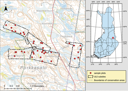
The study site was divided into five subsites with a combined area of 2.4 km². The area of individual subsites varied between 0.4 and 0.6 km². To ensure the abundance of dead trees, the subsites were placed on areas mainly consisting of mature forest with characteristics of old-growth forest, such as a deadwood continuum and uneven age structure. However, the easternmost subsite was located within managed forest and thus somewhat differed from the four other subsites. Some of the western subsites were partially located within Hiidenportti National Park, but most were within state-owned forest connecting the national park to Teeri-Lososuo mire conservation area.

2.2. Field-measured data

The field-measured data consisted of measurements of living and standing dead trees at 37 circular sample plots (radius 9 m) located within the five subsites (see Figure 1). Fourteen of these sample plots were part of a systematic sample plot grid originally designed for the study presented in Heinaro et al. (2021). These plots were inventoried between July and September 2019. The remaining 23 sample plots were placed to known locations of deadwood hotspots and inventoried in November 2020.

The field-measured data included information about the location, height, diameter at breast height (DBH), species, and decay state of each standing dead tree located within the sample plots. The locations were measured in Fix mode with a Trimble R2 (Trimble Inc., Sunnyvale, California, U.S.A.) real-time kinematic (RTK) global navigation satellite system (GNSS) receiver by placing the receiver as close as possible to the tree stem. This resulted in an estimated positional accuracy of less than one metre. The heights were measured with a Vertex 5 measurement device (Haglöf Sweden AB, L°angsele, Sweden), whereas the DBH was measured using steel calipers. The decay state was measured on a scale of 1 to 5 using the guidelines of the Finnish national forest inventory (NFI; Natural Resources Institute Finland 2009). NFI has a separate classification scheme for standing and fallen trees. To ensure the uniformity of measurements, the scheme for fallen trees was used in this study, as the field data were collected during a campaign that inventoried both standing and fallen dead trees. Class 1 represented least decayed trees whereas class 5 represented fully decayed trees. See Appendix A in Heinaro et al. (2021)for a comprehensive description of the decay classes. Table 1 presents a summary of the reference trees. In addition to dead trees, the number of all living trees with a DBH over 45 mm was recorded to calculate the proportion of dead and living trees within the sample plots. The living trees were positioned by measuring the angle and distance from the sample plot centre, but the accuracy of positioning was not sufficient for utilizing this information in the study.

Table 1. Summary statistics of the field-measured standing dead trees, including the minimum (min), mean, maximum (max), and standard deviation for height and diameter at breast height (DBH), and the proportion of trees for each decay class. Note that the decay state classification scheme used in this study was originally intended for fallen trees, and thus very few field-measured trees belonged to decay classes 3–5.

	Total	Scots pine	Norway spruce	Silver and downy birch	Aspen
Number of trees	75	21	43	8	3
Height (m)
Min	1.5	1.5	1.8	4.9	2.4
Mean	11.2	8.4	12.5	12.2	2.4
Max	27.1	21.1	27.1	16.8	2.4
Standard deviation	5.7	5.9	5.3	4.6	0
DBH (mm)
Min	92	107	103	92	190
Mean	194	218	176	196	262
Max	660	660	451	339	362
Standard deviation	93	130	70	73	89
Decay class
Proportion of class 1	81%	86%	84%	63%	67%
Proportion of class 2	17%	14%	14%	38%	33%
Proportion of class 3	1%	0%	2%	0%	0%
Proportion of class 4	0%	0%	0%	0%	0%
Proportion of class 5	0%	0%	0%	0%	0%

2.3. ULS data

The laser scanning data were collected with a Riegl miniVUX-1DL discrete return laser scanner (RIEGL Laser Measurement Systems GmbH, Horn, Austria) mounted on a UAV. To ensure positioning accuracy, the scanner was coupled with a NovAtel CPT7 dual-antenna GNSS-IMU device (Novatel Incorporated, Calgary, Canada). Laser scanning data from each of the five subsites were collected with six to nine flight lines with a 30% overlap. The point density was 285 points/m2 on average. The data were collected in the beginning of June 2020 in mostly leaf-off conditions just after the snow had melted. In addition to three-dimensional coordinates, the dataset included an intensity value for each point.

2.4. Annotated data

The annotated dataset was collected from within the five subsites but from outside the field-measured sample plots. Crowns of standing dead trees were manually identified and digitized from RGB orthoimages (resolution 3.9–4.4 cm) collected using a UAV. The images were acquired in July 2019 with a 20 megapixel complementary metal oxide semiconductor (CMOS) sensor coupled with an RTK GNSS-IMU device (see, DJI 2023) and orthorectified using a digital surface model. The RGB images covered the ULS subsites and field sample plots only partially, and thus the dataset could only be used for the collection of annotated training data, as opposed to utilizing its spectral information in standing dead tree detection. In total, 148 dead trees were identified. Table 2 presents a summary of the annotated data. Note that the heights of the annotated dead trees were determined from the relative heights of the points in the ULS dataset.

Table 2. Summary statistics of the annotated trees, including the minimum (min), mean, maximum (max), and the standard deviation of the heights of the annotation-labelled segments. The heights were determined from the ULS dataset as the heights of the highest point belonging to each segment.

Number of trees	148
Height (m)
Min	6.2
Mean	18.1
Max	28.6
Standard deviation	4.5

2.5. The method for detecting standing dead trees

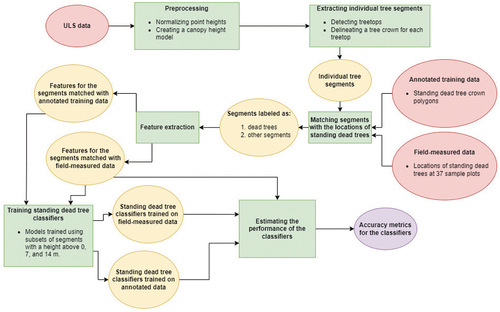
The standing dead tree detection method used in this study was based on multiple steps. First, individual tree segments were detected and delineated from the ULS dataset using a CHM-based segmentation algorithm. Next, a number of features were extracted from each segment. Finally, these features were input into several binary classifiers that labelled the segments as dead or non-dead. The non-dead class included all segments not representing dead trees, such as living trees, shrubs, and segments consisting of multiple trees. Known locations of dead trees were matched with the individual tree segments to acquire training data for the classifiers. Figure 2 presents a summary of the standing dead tree detection process. The following sections describe the steps of the process in more detail.

Figure 2. The standing dead tree detection process.

2.5.1. Data preprocessing

As a first step, ground points were extracted from the laser scanning data using cloth simulation (Zhang et al. 2016). Then, the heights of the points were normalized by creating a triangulated irregular network (TIN) model using the extracted ground points and subtracting the corresponding TIN value from the height of each point. As a result, the height of each point represented the height above ground. Finally, a CHM with a 0.5-metre resolution was generated using the normalized points and the method introduced in Khosravipour et al. (2014), which combines several CHMs generated using different height-based subsets of points to create the final pitfree CHM. All preprocessing steps were performed using R’s lidR package (Roussel and Auty 2022; Roussel et al. 2020) and its readily available functions.

2.5.2. Individual tree detection and delineation

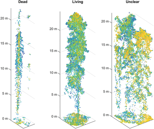
After preprocessing the laser scanning data, individual tree segments were delineated from the point cloud using a CHM-based delineation algorithm. We chose to use a CHM-based algorithm instead of an algorithm operating directly on the point cloud, as CHM-based algorithms are generally less prone to oversegmentation (Wang et al. 2016). First, the treetops were detected from the generated CHM using lidR’s local maximum filter (lmf) algorithm, which is based on the method developed by Popescu and Wynne (2004). The method searches for treetops using variable window sizes that are based on surrounding laser point heights. The intuition behind this method is that the taller the tree, the larger its crown and thus a larger window size should be used when searching for its treetop. After the treetops had been identified, individual tree crowns were delineated around the detected treetops using a region growing based algorithm introduced in Michele et al. (2016). Further in the text, the individual trees extracted from the point clouds will be denoted as laser-derived segments. Figure 3 shows an example of three such segments.

Figure 3. Examples of laser-derived tree segments. The figure shows three segments: a segment representing a dead tree (left), a segment representing a living tree (middle), and a result of unsuccessful segmentation (right). The segment points are colored by intensity with yellow points representing high-intensity points and blue points representing low-intensity points.

2.5.3. Matching laser-derived segments with the annotated crowns and field-measured trees

After individual tree detection and delineation, we had laser-derived segments of all the individual trees in the ULS dataset. In order to enable further analysis, these segments needed to be labelled as dead or non-dead, and they were thus matched with the annotated crowns and field-measured trees. The matching process was slightly different for these two datasets. The following sections describe the matching process for each dataset.

2.5.3.1. Matching tree segments with the annotated crowns

The annotated dataset consisted of digitized crown polygons of standing dead trees. Matching these polygons with the laser-derived segments required calculating the locations of both the annotated crown polygons and the laser-derived tree segments. The location of each crown polygon was calculated as the centroid of the polygon, whereas the location of each tree segment was determined to be the median (x,y)-coordinate of the point cloud points belonging to the segment. Each dead tree represented by an annotated crown polygon was matched with its closest laser-derived tree segment if the locational difference was at most 2 metres. Otherwise, the crown polygon was discarded. This resulted in 148 laser-derived tree segments labelled as standing dead trees. In addition, 592 tree segments not labelled as dead trees were randomly selected, ensuring that these segments were not within the field-measured sample plots. These segments were used as observations of the non-dead class in the annotated dataset. The number of non-dead observations was selected based on the distribution of living and dead trees in the field-measured data in which dead trees covered approximately 20% of the observations. This resulted in some information leakage from the field-measured dataset to the annotated data. However, we assumed that the distribution of dead and living trees would have been similar anywhere within the study site, and thus this information leakage would not significantly bias the results. Note that we refer to the laser-derived tree segments not labelled as dead trees as non-dead segments, as, in addition to representing living trees, they represented incorrect segmentations and other objects in the forest. Table 3 presents a summary of the dead and non-dead laser-derived tree segments in the annotated dataset. Further in the text, the laser-derived segments matched with annotated data will be denoted as annotation-labelled segments.

Table 3. The number of annotation-labelled segments taller than different height thresholds.

Height (m)	Total	Dead	Non-Dead
$\ge 0$	740	148	592
$\ge 7$	670	144	526
$\ge 14$	459	126	333

2.5.3.2. Matching laser-derived tree segments with field-measured trees

The locations of field-measured dead trees were directly available as RTK-measured coordinates. The location of each laser-derived tree segment was determined to be the median (x,y)-coordinate of the point cloud points belonging to the segment. Tree segments were matched with dead field-measured trees in the following way:

1. The field-measured trees were sorted into descending order based on their height.

2. Starting from the tallest field-measured tree, all laser-derived tree segments within 5 meters from the tree were extracted.

3. If there were no tree segments within 5 meters from the tree, the field-measured tree was matched with its closest tree segment. Otherwise, the field-measured tree was matched with the segment whose height was closest to the height of the field-measured tree. The tree segment height was determined as the 98th percentile of the height of the points belonging to the segment.

4. The matched tree segment was removed so that it would not be matched with another field-measured tree.

5. Steps 2 to 4 were repeated for all field-measured trees.

The tree segmentation in the individual tree detection and delineation phase (section 2.5.2) was not perfect and as a result, some trees were represented by several segments and some were grouped together (i.e. over- and undersegmentation). The matching process described above ensured that each dead field-measured tree was matched with the most similar nearby laser-derived tree segment. Furthermore, the matching process ensured that each dead field-measured tree was matched with a laser-derived tree segment. There were a few cases where a dead field-measured tree was matched with a tree segment located more than 5 metres away from the field-measured tree. In these cases, it was unlikely that the match was a true match. However, ensuring a match for each dead field-measured tree simplified validation significantly, as non-matched trees did not have to be handled separately. The matching process resulted in 75 laser-derived tree segments labelled as standing dead trees. All non-matched tree segments located within the sample plots were labelled as non-dead. Table 4 presents a summary of the dead and non-dead laser-derived tree segments in the field-measured dataset. Further in the text, the laser-derived segments matched with field-measured trees will be denoted as field data labelled segments.

Table 4. The number of field data labelled segments in different height, diameter, decay class, and species groups. Note that for non-dead segments, the diameter, decay class, and species could not be determined.

	Total	Dead	Non-Dead
Height (m)
$\ge 0$	367	75	292
$\ge 7$	324	57	267
$\ge 14$	203	23	180
DBH (mm)
$\ge 0$	—	75	—
$\ge 150$	—	48	—
$\ge 250$	—	14	—
Decay class
1	—	61	—
2	—	13	—
3	—	1	—
Species
Scots pine	—	21	—
Norway spruce	—	43	—
Silver and downy birch	—	8	—
Aspen	—	3	—

2.5.4. Feature extraction

At this stage of the standing dead tree detection process, we had laser-derived tree segments labelled as dead or non-dead trees. The next step was to extract features for these segments, which could then be used for training and validating models aiming to classify tree segments as dead or non-dead. In total, 90 features were extracted for each tree segment. Table 5 presents a detailed description of the features. The features can be roughly grouped into 8 classes:

1. Height-related features

2. Intensity-related features

3. Features describing the tree crown

4. Proportions of different point types (single, first, intermediate, last)

5. Proportions of points within different distance intervals from the segment centre

6. Proportional segment widths at different heights

7. Shape feature histograms

8. Other features, including the minimum enclosing circle and fractional cover

Table 5. A description of the features extracted for each tree segment.

Feature type	Description	Number of features
Intensity statistics	The min, max, mean, mode, standard deviation, skewness, kurtosis, 25th percentile, 50th percentile (median), and 75th percentile of the intensities of the points belonging to the segment.	10
Intensity histogram	The proportion of points falling at each of five intensity histogram bins. The bin edges were determined by recording the minimum and maximum intensity of a point belonging to the segment and dividing the interval between these values equally into five bins.	5
Height statistics	The min, max, mean, mode, standard deviation, skewness, kurtosis, 25th percentile, 50th percentile (median), and 75th percentile of the heights of the points belonging to the segment.	10
Height histogram	The proportion of points falling at each of five height histogram bins. The bin edges were determined by recording the minimum and maximum height of a point belonging to the segment and dividing the interval between these values equally into five bins.	5
Crown base height	The estimated crown base height of the segment. Determined by calculating the proportion of points at 0.5 m height intervals and setting the mid-range of the lowest interval containing at least 2% of the segment points as the crown base height.	1
Crown area	The estimated crown area of the segment. Determined as the area of the horizontal convex hull of points above the crown base height.	1
Crown volume	The estimated crown volume of the segment. Determined as the volume of the tightest fitting alpha shape that encloses all points above the crown base height.	1
Maximum crown diameter	The maximum horizontal distance between two points above the crown base height.	1
Fractional cover	The fraction of points above the crown base height.	1
Minimum enclosing circle	The radius of the smallest horizontal circle enclosing all segment points.	1
Proportional width at different heights	The segment is divided into 5 height intervals. Then, the horizontal distances between all point-pairs within each height interval are calculated. The width of a specific height interval is determined as the 95th percentile of the point-pair distances at that height interval. Finally, the width of each height interval is divided by the 95th point-pair distance between all points in the segment to get the proportional width at for each height interval.	5
Point type proportions	The proportion of single, first, intermediate, and last return points in the segment.	4
Proportion of points at different distances from segment centre	All segment points are projected on the xy-plane. The segment centre C is defined as the median (x,y)-coordinate of the points. The furthest distance F from the segment centre is defined as the 95th percentile of the distances from the points to the segment centre. The projected segment is divided into 5 equally spaced distance regions between 0 and C and the proportion of points within each such region is calculated.	5
3D shape feature histogram	For each point in the segment, 8 shape features are calculated using the coordinate covariance matrix of the 6 neighbours of the point. These shape features are linearity, planarity, sphericity, omnivariance, anisotropy, eigenentropy, sum of eigenvalues, and change of curvature (see, e.g. Weinmann (2015) for more information). For each shape feature, a histogram of 5 equally spaced bins is calculated using the values of individual points.	40

2.5.5. Model creation and validation

The extracted features were used for fitting binary classifiers that aimed to predict whether a given tree segment represented a dead tree. All fitted classifiers consisted of the following three steps:

1. Standardizing the features by subtracting the mean and dividing by the standard deviation of the feature.

2. Selecting the K best features to be used in the model. K was a hyperparameter to be optimized. The selection was based on calculating the analysis of variance (ANOVA) F-statistic for each feature (i.e., inspecting how well the feature is able to separate living and dead tree segments) and selecting the K features with the largest values of the F-statistic. The tested values for K were 10–90 features with 10 feature increments.

3. Fitting a logistic regression model using the K selected features and L1 regularization. The strength of regularization was another hyperparameter to be optimized.

Separate classifiers were trained using the annotation-labelled and field data labelled segments. In addition, we used a dummy classifier as a baseline to inspect whether the classifiers achieved a higher performance than random guessing. The dummy classifier randomly predicted whether a tree segment was dead or not based on the proportion of dead and non-dead field data labelled segments. To enable assessing the performance of the classifiers against unseen ground truth, the following cross-validation procedure was used for fitting and validating the classifiers:

1. The annotation-labeled segments were used for training a classifier. Its hyperparameters were optimized using stratified 5-fold cross-validation within the annotated dataset. Stratified cross-validation ensured that the proportion of dead and non-dead samples was retained in the training and validation datasets.

2. The field data labelled segments were split into five subsets ensuring that the proportion of dead and non-dead segments was retained in each subset. (i.e., stratified subsets)

3. One of the five subsets of field data labelled segments was left out as the test set, and a classifier was fit to the remaining four subsets of segments. The hyperparameters of this classifier were optimized using 5-fold stratified cross-validation. A dummy classifier was also trained using the proportion of dead and non-dead tree segments in the four subsets of field data labelled segments.

4. The left out test set was used for evaluating the performance of the classifiers. The precision, recall, Cohen’s kappa score (Cohen 1960), and Matthews correlation coefficient (MCC, Matthews 1975) were calculated for each classifier.

5. Steps 3–4 were repeated five times, so that each of the five subsets of field data labelled segments was used as the test set.

6. Steps 2–5 were repeated 100 times with different random subsets of field data labelled segments, and the mean performance of each classifier was recorded. This ensured that the results were not dependent on the random splits of the segments. To summarize, the whole validation process consisted of 100 repeats of stratified 5-fold cross-validation.

The optimal hyperparameter selection for the classifiers was based on the area under the precision-recall curve (AUPRC), which inspects how the precision and recall of a classifier change when the classification threshold is changed. Simply put, using AUPRC as the evaluation metric is equivalent to finding a model that aims to correctly identify as many dead trees as possible while minimizing the number of false detections.

The process described above was repeated three times, each time using only the segments taller than a specified height threshold (referred to as the training height threshold further in the text). The training height thresholds used were 0, 7, and 14 metres. The thresholds were selected so that even the classifiers using only the tallest tree segments would contain a sufficient number of training samples. As a result, we had three classifiers utilizing annotation-labelled segments, three classifiers utilizing field data labelled segments, and three dummy classifiers. Table 3 presents the number of annotation-labelled segments taller than each height threshold. Similarly, Table 4 presents the number of field data labelled segments taller than each height threshold.

2.5.6. Estimating feature importance

Due to the relatively complex cross-validation scheme, we chose to estimate feature importance using coefficient values. Since the features were normalized, the magnitude of a coefficient provided a rough estimate of the predictive power of the corresponding feature. The estimation of feature importance was based on mean coefficient values across classifiers fitted during different cross-validation folds.

3. Results

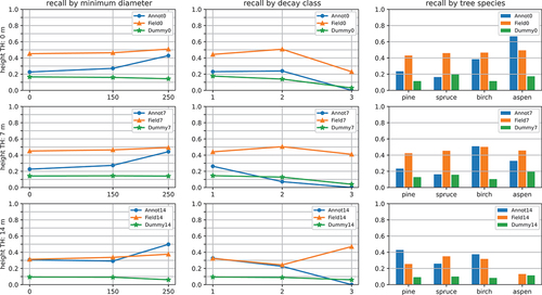
In general, the classifiers trained using annotation-labelled segments or field data labelled segments were able to outperform random guessing, as they beat the dummy models in most cases, and their MCC and kappa scores were larger than zero. However, the performance was rather modest, as the highest MCC and kappa scores the classifiers were able to achieve were 0.20 and 0.17 for the model trained on annotation-labelled segments, and 0.13 and 0.08 for the model trained on field data labelled segments. Figures 4 and 5 show the performance of the classifiers on trees of different heights, diameters, decay classes, and species. Each row of plots presents results for the classifiers trained using segments taller than a specific height threshold. The height-specific results in Figure 4 include precisions, recalls, Cohen’s kappa scores, and MCCs. The diameter, decay class, and species-specific results (Figure 5) only include recalls, as these characteristics could not be determined for false positives (tree segments that were falsely classified as dead).

The figures show that the performance of the classifiers increased as tree height and diameter increased. This phenomenon was especially evident with the models trained on annotation-labelled segments, whose performance improved significantly when only inspecting the largest trees (trees with a height above 14 m or diameter above 250 mm). As a result, the performance of the annotation-based classifiers was mainly higher with large trees compared to the classifiers trained on field data labelled segments.

Increasing the training height threshold did not improve the performance of the classifiers. In fact, the performance of the classifiers trained on annotation-labelled segments generally decreased as the training height threshold increased. The threshold did not seem to significantly impact the performance of the classifiers trained on field data labelled segments.

The decay state and species-specific results were rather mixed. There was no clear trend between different tree species, decay classes, and the performance of different classifiers. This implies that other tree attributes, such as height and diameter were more significant factors regarding performance.

Figure 4. The results of different classifiers for trees of different heights. Each row of plots shows the results for the classifiers trained using tree segments taller than a specific height threshold (height TH). AnnotX, FieldX, and DummyX denote the classifier trained using annotation-labeled segments, the classifier trained using field data labeled segments, and the dummy classifier, respectively. The plots show the precision, recall, Cohen’s kappa ($\kappa$), and Matthews correlation coefficient (MCC) on trees larger than 0, 7, and 14 meters. Refer to Table 4 for the number of observations in each of these height classes. Note that the scales of the y-axes differ between different plot columns.

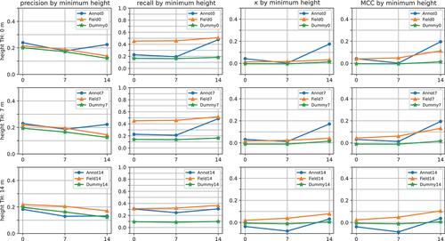
Figure 5. The recalls of different classifiers for trees of different diameters decay classes and species Each row of plots shows the results for the classifiers trained using tree segments taller than a specific height threshold (height TH). AnnotX, FieldX, and DummyX denote the classifier trained using annotation-labeled segments, the classifier trained using field data labeled segments, and the dummy classifier, respectively. In the left column, each data point represents the proportion of trees with a diameter larger than the specified diameter detected with the method. In the latter two columns, each data point represents the proportion of trees in a specific decay class/tree species detected with the method. Note that recalls for decay classes 4 and 5 are excluded, as the reference dataset contained no trees belonging to these classes. Refer to Table 4 for the number of observations in each of the diameter and decay classes, and tree species.

Table 6 shows the five most important features of each model according to coefficient magnitudes. We see that height- and intensity-related features were the most important for the classifiers trained on annotated segments. In contrast, classifiers trained on field data also utilized features describing the horizontal geometric properties of the segments.

Table 6. The five most important features for each classifier, based on the coefficient magnitudes. AnnotX denotes the classifier trained using annotation-labelled segments taller than X metres, whereas FieldX denotes the classifier trained using field data labelled segments taller than X metres. $H_{max}$, $H_{mean}$, $H_{kurt}$ represent the maximum, mean, and kurtosis of the heights of the points belonging to a segment, whereas $H_{M\mathrm{\%}}$ and $H_{binN}$ denote the Mth percentile and Nth histogram bin of the segment heights, respectively. $I_{std}$, $I_{skew}$, and $I_{M\mathrm{\%}}$ represent the standard deviation, skewness, and Mth percentile of the intensities of the segment points. $C{D}_{max}$ and $MEC$ denote the maximum crown diameter and minimum enclosing circle of the segment, whereas $PT{P}_{intermediate}$ denotes the proportion of intermediate echoes in the segment. $E{E}_{binM}$ and $C{C}_{binN}$ represent the Mth and Nth bin of the shape feature histograms describing the eigenentropy and change of curvature of the segment. $PDis{t}_{binM}$ represents the proportion of points within the Mth horizontal distance bin from the segment centre. See Table 5 for a more detailed description of the features.

	Annot0	Annot7	Annot14	Field0	Field7	Field14
1	$H_{max}$	$H_{max}$	$H_{max}$	$C{D}_{max}$	$I_{std}$	$I_{skew}$
2	$H_{75\mathrm{\%}}$	$H_{75\mathrm{\%}}$	$I_{75\mathrm{\%}}$	$H_{mean}$	$C{D}_{max}$	$H_{kurt}$
3	$H_{bin5}$	$H_{75\mathrm{\%}}$	$PT{P}_{intermediate}$	$PDis{t}_{bin5}$	$C{C}_{bin2}$	$H_{25\mathrm{\%}}$
4	$H_{50\mathrm{\%}}$	$I_{25\mathrm{\%}}$	$H_{75\mathrm{\%}}$	$E{E}_{bin5}$	$H_{mean}$	$PDis{t}_{bin4}$
5	$I_{25\mathrm{\%}}$	$I_{50\mathrm{\%}}$	$H_{50\mathrm{\%}}$	$MEC$	$E{E}_{bin5}$	$H_{bin2}$

4. Discussion

This study inspected the effects of using image-annotated training data in ULS-based standing dead tree detection. Furthermore, the study examined whether ULS-based standing dead tree detection should focus on large trees. The study was carried out by comparing the performances of classifiers trained on annotation-labelled segments and field data labelled segments.

The results of this study showed that annotation-based classifiers were able to correctly label a larger proportion of large trees compared to classifiers trained on field data labelled segments. This was true for all classifiers except the ones trained with segments over 14 m tall, with which the annotation-based classifier suffered from the decrease in the number of training samples. Comparing Tables 1 and 2 reveals that the trees in the annotated dataset were, on average, significantly larger than those in the field dataset. This likely explains the better performance of annotation-based classifiers on large trees at least partially, as classifiers learn to label samples similar to the ones they were trained on.

Against the hypothesis of this study, it seemed that using a height threshold for the segments used as training data did not improve performance. For the annotation-labelled segments, performance actually decreased, whereas for the field data labelled segments, performance remained similar regardless of the training height threshold used. There are two contradicting factors that impact performance when filtering training segments based on their height. Firstly, as hypothesized, tree segments representing large trees are more likely accurate representations, whereas small tree segments might contain coarse segmentation errors. Thus, filtering segments based on their height should remove some of the non-representative dead tree segments while retaining most of the representative ones. This should improve the performance of the classifier. Secondly, when the training height threshold is increased, the number of training segments decreases, which likely impairs the classification performance. Based on the results, it seems that the increase in representativeness was not able to outweigh the decrease in the number of training segments. It seems that most of the annotation-labelled training segments were somewhat representative regardless of their height, and thus filtering these segments only impaired performance. Intuitively, this makes sense, as the dead trees in the annotated dataset must have all been visible in the RGB images from which they were identified. This implies that the dead trees likely had some sort of crown and that they were not hidden under the canopies of other trees. Such a setting indicates that the trees were likely visible and easily separable in the ULS dataset as well.

The study showed that large dead trees (length- and diameter-wise) were detected with a higher accuracy than small dead trees. Similar results were shown by Wing et al. (2015). This rather expected result is likely due to small trees often being surrounded by larger trees that hide the small trees underneath them. This impacts the detection of small dead trees in three ways. Firstly, small trees might simply not be visible in the point cloud, making their detection impossible. Secondly, even if a small tree is present in the point cloud, the rule-based individual tree segmentation algorithm might miss the tree, as it is surrounded by larger trees that clearly stand out in the point cloud. This problem is even more evident with CHM-based segmentation algorithms, as they identify treetops from a CHM that only describes the uppermost canopy layer. Thirdly, even if the individual tree segmentation algorithm is able to detect a small tree, the extracted segment might not be an accurate representation of the tree, as branches of surrounding large trees are included in the segment. As a result, the geometry-based features derived from the segment are distorted and thus the segment can not be correctly labelled during the classification phase.

While large dead trees are generally considered to have the most ecological significance, being able to map small dead trees would be beneficial, as they contribute to the total deadwood volume. Based on the results of this study, it seems that detecting individual small dead trees is rather challenging using remote sensing data collected from above the canopy. Thus, one option to improve the comprehensiveness of deadwood inventories would be to use devices that enable data collection from beneath the canopy, such as terrestrial laser scanning (TLS) or mobile laser scanning (MLS) (see, e.g. Yrttimaa et al. 2019). The significant downside of such an approach is that it is not suited for large-scale monitoring. Another approach for incorporating small dead trees in deadwood inventory would be to use indirect methods that model the relationship between directly measurable remote sensing attributes and field-measured dead trees (see, Bater et al. 2009; Jon and King 2009). However, this approach has proven challenging as well due to the scattered occurrence of deadwood.

Overall, the performance of the classifiers was rather poor, which indicates that there was a weak connection between the training segments and test segments. This was especially true for the classifiers trained on field data labelled segments, which performed rather weakly with trees of all sizes. One reason for this might be that the features used were not suitable for distinguishing dead tree segments from other segments. A perhaps more probable explanation is that a large fraction of the segments in the point cloud simply did not accurately represent individual trees. A visual inspection of the segments revealed that a significant fraction of both dead and non-dead segments resembled something similar to the right-most segment in Figure 3, which represents a segment consisting of multiple trees. Such segments were formed due to several trees being very close to each other and are rather challenging to eliminate regardless of the individual tree segmentation method used. Wing et al. (2015) and Yao, Krzystek, and Heurich (2012) mentioned that the success of individual tree segmentation is crucial for standing dead tree detection. The results of this study support this observation. Finding a suitable segmentation algorithm and optimizing its parameters is rather challenging, as the conditions in the forest can vary even within a small area. Shifting from the individual tree segmentation and classification based approach to direct object detection (see, e.g. Lang et al. 2019; Zhou and Tuzel 2017) would potentially solve this issue, as object detection removes the need for the segmentation phase. However, the disadvantage of object detection is that it requires a large amount of training data, and thus it was not used in this study.

The study setting had limitations that might have impacted the results. Firstly, the field dataset was smaller than the annotated dataset, which possibly favoured the classifiers trained on the annotation-labelled segments. The annotation-labelled segments could have been sub-sampled to balance the number of samples in both datasets. However, we chose not to do so, as the possibility of collecting a large number of training samples efficiently is the main advantage of annotated data. Furthermore, the classifiers trained on field data labelled segments did not seem to be very sensitive to the number of training samples, as the performance remained similar regardless of the training height threshold used. Secondly, logistic regression was used as the classifier. Logistic regression is not able to learn interactions between features unless interaction features are explicitly crafted. Furthermore, logistic regression suffers from collinearities between features. Using more complex classifiers inherently capable of handling interactions and collinearities between features might have proven beneficial. However, such methods are more prone to overfitting, which is a concern especially with the somewhat limited field dataset. Thirdly, the segment matching process used for the field dataset ensured that each dead field-measured tree was matched with a laser-derived tree segment. Using such a matching procedure simplified performance evaluation, as it eliminated the need for separately inspecting whether a field-measured dead tree was matched or not and whether it was correctly identified as a dead tree. However, it is likely that with this matching procedure, a few of the field-measured trees were matched with a tree segment that in reality represented another tree. With the small dataset used in this study, a manual matching procedure could have mitigated this issue. Fourthly, the data annotations were collected by a single person, which introduced some subjectivity to the results. Visually identifying crowns of dead trees from aerial images is not a trivial task, and the annotations provided by different annotators would likely differ from each other. Our annotator was experienced and likely identified most types of dead trees visible in the RGB dataset. Furthermore, the high resolution of the RGB dataset minimized ambiguity in the annotation process. Still, combining the annotations of multiple annotators (see, e.g. Schmarje et al. 2022; Yan et al. 2014) would have reduced the subjectivity of the results.

5. Conclusions

This study suggested that airborne laser scanning based standing dead tree detection should focus on detecting large dead trees, as most small dead trees can simply not be identified and correctly segmented even from high density point clouds. Thus, using annotated training data is a viable option even if small dead trees are underrepresented in such data. The study identified the rule-based individual tree segmentation phase as the single most error-prone step of standing dead tree detection. More research should be focused on inspecting the suitability of different individual tree segmentation methods for segmenting dead trees, as thus far, research on the topic has mainly focused on living trees. To take a step further, future studies could inspect the possibility of eliminating the rule-based individual tree detection phase altogether, and shifting to direct object detection. Annotated data could prove useful in such an approach, as annotation enables collecting large training datasets more efficiently that field measurements.

Acknowledgements

The authors would like to thank Osmo Suominen and Aleksi Ritakallio for helping with field data collection, and Max Strandén for the annotations.

Disclosure statement

No potential conflict of interest was reported by the author(s).

Data Availability statement

The data that support the findings of this study are available from the corresponding author, E.H., upon reasonable request.

Additional information

Funding

This work was supported by the Doctoral Program in Sustainable Use of Renewable Natural Resources (AGFOREE) at the University of Helsinki; the LIFE financial instrument of the European Union [LIFE17/NAT/FI/000181]; the Academy of Finland’s Strategic Research Council [312559]; and the Academy of Finland’s Research Council for Natural Sciences and Engineering [334829]. Open access funding provided by the University of Helsinki.

References

- Amiri, N., P. Krzystek, M. Heurich, and A. Skidmore. 2019. “Classification of Tree Species as Well as Standing Dead Trees Using Triple Wavelength ALS in a Temperate Forest.” Remote Sensing 11 (22): 2614. https://doi.org/10.3390/rs11222614.
- Bater, C. W., N. C. Coops, S. E. Gergel, V. LeMay, and D. Collins. 2009. “Estimation of Standing Dead Tree Class Distributions in Northwest Coastal Forests Using Lidar Remote Sensing.” Canadian Journal of Forest Research 39 (6): 1080–1091. https://doi.org/10.1139/X09-030.
- Beucher, S. 1979. “Use of Watersheds in Contour Detection.” In Proceedings of the International Workshop on Image Processing, CCETT.
- Bradford, J., P. Weishampel, M.-L. Smith, R. Kolka, R. A. Birdsey, S. V. Ollinger, and M. G. Ryan. 2009. “Detrital Carbon Pools in Temperate Forests: Magnitude and Potential for Landscape-Scale Assessment.” Canadian Journal of Forest Research 39 (4): 802–813. https://doi.org/10.1139/X09-010.
- Briechle, S., P. Krzystek, and G. Vosselman. 2020. “Classification of Tree Species and Standing Dead Trees by Fusing UAV-Based LiDar Data and Multispectral Imagery in the 3D Deep Neural Network Pointnet++.” ISPRS Annals of the Photogrammetry, Remote Sensing & Spatial Information Sciences 2:203–210. https://doi.org/10.5194/isprs-annals-V-2-2020-203-2020.
- Casas, Á., M. García, R. B. Siegel, A. Koltunov, C. Ramírez, and S. Ustin. 2016. “Burned Forest Characterization at Single-Tree Level with Airborne Laser Scanning for Assessing Wildlife Habitat.” Remote Sensing of Environment 175:231–241. https://doi.org/10.1016/j.rse.2015.12.044.
- Cohen, J. 1960. “A Coefficient of Agreement for Nominal Scales.” Educational and Psychological Measurement 20 (1): 37–46. https://doi.org/10.1177/001316446002000104.
- DJI. 2023. Phantom 4 - Product Information. Accessed June 4, 2023. https://www.dji.com/fi/phantom-4/info.
- Harmon, M. E., W. K. Ferrell, and J. F. Franklin. 1990. “Effects on Carbon Storage of Conversion of Old-Growth Forests to Young Forests.” Science 247 (4943): 699–702. https://doi.org/10.1126/science.247.4943.699.
- Heinaro, E., T. Tanhuanpää, T. Yrttimaa, M. Holopainen, and M. Vastaranta. 2021. “Airborne Laser Scanning Reveals Large Tree Trunks on Forest Floor.” Forest Ecology and Management 491:119225. https://doi.org/10.1016/j.foreco.2021.119225.
- Hyyppa, J., O. Kelle, M. Lehikoinen, and M. Inkinen. 2001. “A Segmentation-Based Method to Retrieve Stem Volume Estimates from 3-D Tree Height Models Produced by Laser Scanners.” IEEE Transactions on Geoscience and Remote Sensing 39 (5): 969–975. https://doi.org/10.1109/36.921414.
- Jon, P., and D. J. King. 2009. “Mapping Dead Wood Distribution in a Temperate Hardwood Forest Using High Resolution Airborne Imagery.” Forest Ecology and Management 258 (7): 1536–1548. https://doi.org/10.1016/j.foreco.2009.07.009.
- Kamińska, A., M. Lisiewicz, K. Stereńczak, B. Kraszewski, and R. Sadkowski. 2018. “Species-Related Single Dead Tree Detection Using Multi-Temporal ALS Data and CIR Imagery.” Remote Sensing of Environment 219:31–43. https://doi.org/10.1016/j.rse.2018.10.005.
- Khosravipour, A., A. K. Skidmore, M. Isenburg, T. Wang, and Y. A. Hussin. 2014. “Generating Pit-Free Canopy Height Models from Airborne Lidar.” Photogrammetric Engineering & Remote Sensing 80 (9): 863–872. https://doi.org/10.14358/PERS.80.9.863.
- Lang, A. H., S. Vora, H. Caesar, L. Zhou, J. Yang, and O. Beijbom. 2019. ”PointPillars: Fast Encoders for Object Detection from Point Clouds.” digital preprint arXiv:1812.05784. https://doi.org/10.48550/arXiv.1812.05784.
- Lassauce, A., Y. Paillet, H. Jactel, and C. Bouget. 2011. “Deadwood as a Surrogate for Forest Biodiversity: Meta-Analysis of Correlations Between Deadwood Volume and Species Richness of Saproxylic Organisms.” Ecological Indicators 11 (5): 1027–1039. https://doi.org/10.1016/j.ecolind.2011.02.004.
- Martinuzzi, S., L. A. Vierling, W. A. Gould, M. J. Falkowski, J. S. Evans, A. T. Hudak, and K. T. Vierling. 2009. “Mapping Snags and Understory Shrubs for a LiDar-Based Assessment of Wildlife Habitat Suitability.” Remote Sensing of Environment 113 (12): 2533–2546. https://doi.org/10.1016/j.rse.2009.07.002.
- Matthews, B. W. 1975. “Comparison of the Predicted and Observed Secondary Structure of T4 Phage Lysozyme.” Biochimica et Biophysica Acta (BBA) - Protein Structure 405 (2): 442–451. https://doi.org/10.1016/0005-2795(75)90109-9.
- Michele, D., D. A. Coomes, and D. Murrell. 2016. “Tree-Centric Mapping of Forest Carbon Density from Airborne Laser Scanning and Hyperspectral Data.” Methods in Ecology and Evolution 7 (10): 1236–1245. https://doi.org/10.1111/2041-210X.12575.
- Milto, M., A. Agapiou, S. Gonzalez Aracil, and D. G. Hadjimitsis. 2020. “Detecting Dead Standing Eucalypt Trees from Voxelised Full-Waveform Lidar Using MultiScale 3D-Windows for Tackling Height and Size Variations.” Forests 11 (2): 161. https://doi.org/10.3390/f11020161.
- Morsdorf, F., E. Meier, B. Allgöwer, and D. Nüesch. 2003. “Clustering in Airborne Laser Scanning Raw Data for Segmentation of Single Trees.” The International Archives of the Photogrammetry, Remote Sensing and Spatial Information Sciences 34(3):W13.
- Mücke, W., B. Deák, A. Schroiff, M. Hollaus, and N. Pfeifer. 2013. “Detection of Fallen Trees in Forested Areas Using Small Footprint Airborne Laser Scanning Data.” Canadian Journal of Remote Sensing 39 (sup1): S32–S40. https://doi.org/10.5589/m13-013.
- Natural Resources Institute Finland. 2009. VMI11. In Finnish, Accessed March 20, 2019. https://jukuri.luke.fi/bitstream/handle/10024/532024/vmi11-maasto-ohje09-2p.pdf?sequence=1isAllowed=y.
- Nyström, M., H. Johan, E. S. F. Johan, and H. Olsson. 2014. “Detection of Windthrown Trees Using Airborne Laser Scanning.” International Journal of Applied Earth Observation and Geoinformation 30:21–29. https://doi.org/10.1016/j.jag.2014.01.012.
- Persson, A., J. Holmgren, and U. Soderman. 2002. “Detecting and Measuring Individual Trees Using an Airborne Laser Scanner.” Photogrammetric Engineering and Remote Sensing 68 (9): 925–932.
- Pesonen, A., M. Maltamo, K. Eerikäinen, and P. Packalèn. 2008. “Airborne Laser Scanning-based Prediction of Coarse Woody Debris Volumes in a Conservation Area.” Forest Ecology and Management 255 (8): 3288–3296. https://doi.org/10.1016/j.foreco.2008.02.017.
- Polewski, P., W. Yao, M. Heurich, P. Krzystek, and U. Stilla. 2015a. “Active Learning Approach to Detecting Standing Dead Trees from ALS Point Clouds Combined with Aerial Infrared Imagery.” In 2015 IEEE Conference on Computer Vision and Pattern Recognition Workshops (CVPRW), Boston, MA, USA, 10–18.
- Polewski, P., W. Yao, M. Heurich, P. Krzystek, and U. Stilla. 2015b. “Free Shape Context Descriptors Optimized with Genetic Algorithm for the Detection of Dead Tree Trunks in ALS Point Clouds.” ISPRS Annals of the Photogrammetry, Remote Sensing & Spatial Information Sciences II-3/W5:41–48. https://doi.org/10.5194/isprsannals-II-3-W5-41-2015.
- Polewski, P., W. Yao, M. Heurich, P. Krzystek, and U. Stilla. 2018. “Learning a Constrained Conditional Random Field for Enhanced Segmentation of Fallen Trees in ALS Point Clouds.” ISPRS Journal of Photogrammetry and Remote Sensing. 140:33–44. Geospatial Computer Vision https://doi.org/10.1016/j.isprsjprs.2017.04.001.
- Popescu, S., and R. Wynne. 2004. “Seeing the Trees in the Forest: Using Lidar and Multispectral Data Fusion with Local Filtering and Variable Window Size for Estimating Tree Height.” Photogrammetric Engineering & Remote Sensing 70 (5): 589–604. https://doi.org/10.14358/PERS.70.5.589.
- Reitberger, J., C. Schnörr, P. Krzystek, and U. Stilla. 2009. “3D Segmentation of Single Trees Exploiting Full Waveform LIDAR Data.” Isprs Journal of Photogrammetry & Remote Sensing 64 (6): 561–574. https://doi.org/10.1016/j.isprsjprs.2009.04.002.
- Roussel, J.-R., and D. Auty. 2022. Airborne LiDar Data Manipulation and Visualization for Forestry Applications. R Package Version 4.0.1, https://cran.r-project.org/package=lidR.
- Roussel, J.-R., A. David, C. C. Nicholas, T. Piotr, R. H. G. Tristan, A. S. Meador, J.-F. Bourdon, F. de Boissieu, and A. Alexis. 2020. “lidR: An R Package for Analysis of Airborne Laser Scanning (ALS) Data.” Remote Sensing of Environment 251:112061. https://doi.org/10.1016/j.rse.2020.112061.
- Schmarje, L., V. Grossmann, C. Zelenka, S. Dippel, R. Kiko, M. Oszust, M. Pastell, et al. 2022. Is One Annotation Enough? - a Data-Centric Image Classification Benchmark for Noisy and Ambiguous Label Estimation. In Advances in Neural Information Processing Systems, edited by S. Koyejo, S. Mohamed, A. Agarwal, D. Belgrave, K. Cho, and A. Oh, Vol. 35 33215–33232. Curran Associates, Inc. https://proceedings.neurips.cc/paperfiles/paper/2022/file/d6c03035b8bc551f.474f040fe8607cab−Paper−DatasetsandBenchmarks.pdf.
- Stokland, J. N., J. Siitonen, and B. Gunnar Jonsson. 2012. Biodiversity in Dead Wood. Ecology, Biodiversity and Conservation. Cambridge University Press.
- Tanhuanpää, T., V. Kankare, M. Vastaranta, N. Saarinen, and M. Holopainen. 2015. “Monitoring Downed Coarse Woody Debris Through Appearance of Canopy Gaps in Urban Boreal Forests with Bitemporal ALS Data.” Urban Forestry & Urban Greening 14 (4): 835–843. https://doi.org/10.1016/j.ufug.2015.08.005.
- Vauhkonen, J., M. Maltamo, R. E. McRoberts, and E. Næsset. 2014. Introduction to Forestry Applications of Airborne Laser Scanning. Forestry Applications of Airborne Laser Scanning: Concepts and Case Studies, 1–16. Dordrecht, Netherlands: Springer Netherlands. https://doi.org/10.1007/978-94-017-8663-8_1
- Vincent, L., and P. Soille. 1991. “Watersheds in Digital Spaces: An Efficient Algorithm Based on Immersion Simulations.” IEEE Transactions on Pattern Analysis and Machine Intelligence 13 (6): 583–598. https://doi.org/10.1109/34.87344.
- Wang, Y., J. Hyyppä, X. Liang, H. Kaartinen, Y. Xiaowei, E. Lindberg, J. Holmgren, et al. 2016. “International Benchmarking of the Individual Tree Detection Methods for Modeling 3-D Canopy Structure for Silviculture and Forest Ecology Using Airborne Laser Scanning.” IEEE Transactions on Geoscience and Remote Sensing 54 (9): 5011–5027. https://doi.org/10.1109/TGRS.2016.2543225.
- Wehr, A., and U. Lohr. 1999. “Airborne Laser Scanning—An Introduction and Overview.” ISPRS Journal of Photogrammetry and Remote Sensing 54 (2): 68–82. https://doi.org/10.1016/S0924-2716(99)00011-8.
- Weinmann, M., Jutzi, B., Hinz, S, and Mallet C. 2015. ”Semantic point cloud interpretation based on optimal neighborhoods, relevant features and efficient classifiers.” ISPRS Journal of Photogrammetry and Remote Sensing 105: 286–304. https://doi.org/10.1016/j.isprsjprs.2015.01.016.
- Wenkai, L., Q. Guo, M. K. Jakubowski, and M. Kelly. 2012. “A New Method for Segmenting Individual Trees from the Lidar Point Cloud.” Photogrammetric Engineering & Remote Sensing 78 (1): 75–84. https://doi.org/10.14358/PERS.78.1.75.
- Wing, B. M., M. W. Ritchie, K. Boston, W. B. Cohen, and M. J. Olsen. 2015. “Individual Snag Detection Using Neighborhood Attribute Filtered Airborne Lidar Data.” Remote Sensing of Environment 163:165–179. https://doi.org/10.1016/j.rse.2015.03.013.
- Xingcheng, L., Q. Guo, L. Wenkai, and J. Flanagan. 2014. “A Bottom-Up Approach to Segment Individual Deciduous Trees Using Leaf-Off Lidar Point Cloud Data.” ISPRS Journal of Photogrammetry and Remote Sensing 94:1–12. https://doi.org/10.1016/j.isprsjprs.2014.03.014.
- Yan, Y., R. Rosales, G. Fung, R. Subramanian, and D. Jennifer. 2014. “Learning from Multiple Annotators with Varying Expertise.” Machine Learning 95 (3): 291–327. https://doi.org/10.1007/s10994-013-5412-1.
- Yao, W., P. Krzystek, and M. Heurich. 2012. “Identifying Standing Dead Trees in Forest Areas Based on 3D Single Tree Detection from Full Waveform Lidar Data.” ISPRS Annals of the Photogrammetry, Remote Sensing & Spatial Information Sciences I-7:359–364. https://doi.org/10.5194/isprsannals-I-7-359-2012.
- Yrttimaa, T., N. Saarinen, V. Luoma, T. Tanhuanpää, V. Kankare, X. Liang, J. Hyyppä, M. Holopainen, and M. Vastaranta. 2019. “Detecting and Characterizing Downed Dead Wood Using Terrestrial Laser Scanning.” ISPRS Journal of Photogrammetry and Remote Sensing 151:76–90. https://doi.org/10.1016/j.isprsjprs.2019.03.007.
- Zhang, W., Q. Jianbo, P. Wan, H. Wang, D. Xie, X. Wang, and G. Yan. 2016. “An Easy-To-Use Airborne LiDar Data Filtering Method Based on Cloth Simulation.” Remote Sensing 8 (6): 501. https://doi.org/10.3390/rs8060501.
- Zhou, Y., and O. Tuzel. 2017. ”VoxelNet: End-to-End Learning for Point Cloud Based 3D Object Detection.” digital preprint arXiv:1711.06396. https://doi.org/10.48550/arXiv.1711.06396.