Georeferencing of terrestrial radar images in geomonitoring using kernel correlation

ABSTRACT

Terrestrial radar interferometry (TRI) provides accurate observations of displacements in the line-of-sight (LOS) direction and is therefore used in various monitoring applications. However, relating these displacements directly to the 3d world is challenging due to the particular imaging process. To address this, the radar results are projected onto a 3d model of the monitored area, requiring georeferencing of the 3d model and radar observation. However, georeferencing relies on manual alignment and resource-intensive on-site measurements. Challenges arise from the significant disparity in spatial resolution between radar images and 3d models, the absence of identifiable common natural features and the relationship between image and spatial coordinates depending on the topography and instrument pose. Herein, we propose a method for data-driven, automatic and precise georeferencing of TRI images without the need for manual interaction or in situ installations. Our approach (i) uses the radar amplitudes from the TRI images and the angle of incidence based on the 3d point cloud to identify matching features in the datasets, (ii) estimates the best-fitting transformation parameters using Kernel Density Correlation (KDC) and (iii) requires only rough initial approximations of the radar instrument’s pose. Additionally, we present the correct relation between cross-range and azimuth for ground-based radar instruments. We demonstrate the application on a geomonitoring case using TRI data and a point cloud of a large rock cliff. The results show that the positions of the radar image can be localized in the monitored 3d space with a precision of a few metres at distances of over $1\mathrm{k}\mathit{m}$. This is an improvement of almost one order of magnitude compared to what had been achieved using standard approaches and direct observation of the radar instrument’s pose. The proposed method thus contributes to the automation of TRI data processing and improved localization of small-scale deformation areas detected in radar images.

KEYWORDS:

• GB-SAR
• RAR
• real aperture radar
• LiDAR
• mapping
• cross-range
• point cloud

1. Introduction

Terrestrial radar interferometry (TRI) is a method for deformation monitoring and is especially interesting due to the technical potential of providing highly accurate displacement observations with high temporal resolution. In the last years, an increased number of application cases showed the applicability for monitoring natural scenes like landslides (Pieraccini et al. 2003; Tarchi et al. 2003), rockfalls (Carlà et al. 2019; Kos et al. 2013), glaciers (Margreth et al. 2017; Preiswerk et al. 2016; Riesen et al. 2011) or open pit mines (Reeves et al. 2000) as well as for monitoring of large infrastructure objects such as dams (Alba et al. 2008; Tarchi et al. 1999; Werner et al. 2017; Wieser et al. 2020), bridges (Maizuar et al. 2017; Stabile et al. 2013) and wind turbines (Li, Bhalla, and Ling 2014; Muñoz-Ferreras et al. 2016). Typical instruments used for TRI are Ground-Based Synthetic Aperture Radar (GB-SAR) or terrestrial Real Aperture Radar (RAR).

The common basic result of a radar observation is a single look complex (SLC), which represents the observed scenery sampled with the system’s specific range and cross-range resolution. Each SLC image pixel contains the amplitude and phase which encode the power of the radar signals received after reflection at the corresponding surfaces and the weighted distance of these surfaces in complex form. In an interferometric survey, temporally separated SLCs are evaluated pairwise and the resulting interferogram is used to assess the deformation over the respective time interval (temporal baseline).

For TRI observations, the interpretation of the interferograms is not straightforward, due to the complex interaction of the radar signal with the 3d scene, and therefore mostly needs expert knowledge for the correct interpretation. The difficulty of the interpretation is increased when topographically or geometrically complex scenes are measured (e.g. for steep cliffs or near-vertical dams), resulting in overlay and foreshortening. Georeferencing provides the possibility to visualize the interferometric observations in 3d and thus deformations, allowing for easier interpretation and communication with non-radar experts. However, due to the missing geometrical baseline of most TRI systems direct 3d mapping of interferometric observations using only the radar measurements is not possible (Monserrat 2012). The common solution is to project the radar images onto a 3d terrain model provided, e.g. as a point cloud, surface mesh or digital elevation model (DEM). These are often acquired in practice using different mapping techniques such as photogrammetry or laser scanning, applied concurrently with the radar data acquisitions or in sufficient temporal proximity to them.

To project the 2d radar data into 3d space, several methods are presently described in the literature. Whereas direct absolute georeferencing of the radar instrument by geodetic measurement (GNSS or total station) of the position and orientation is possible, for absolute geocoding they are insufficient (Rebmeister et al. 2022). Tapete et al. (2013) select corresponding features in the radar image and a point cloud manually during the initial georeferencing phase and apply the resulting similarity transformation with parameters estimated in a least-squares sense from these correspondences to the subsequently collected radar images. Cai et al. (2021) and Caduff and Rieke-Zapp (2014) base the georeferencing on markers (e.g. corner reflectors) placed in the region of interest before the measurement and manually detected them in the 2d TRI image and 3d model. For solving the transformation problem based on these established marker correspondences, a least-squares approach is commonly used.

However, all the aforementioned works rely on a precise initial position and orientation information of the TRI instrument and sometimes on additional ground control points distributed within the area of observation. These are typically acquired by a geodetic survey using RTK GNSS or a total station and the installation of in situ ground control points can be difficult, especially if accessing the area may be dangerous or has limited possibilities for access.

The main objective of this paper is to introduce an approach for automatic and precise georeferencing of TRI images using a 3d point cloud, without the need for precise prior knowledge of the radar pose and without detection of corresponding features in the scenery. In this paper, we use the point cloud as a 3d surface model of the monitored area, and the presented approach is also applicable if the surface model is available in a different form initially, e.g. as a mesh, DEM or parametric surface model like a NURBS surface. In these cases, the nodes of the mesh or the grid points of the DEM can be used directly as a point cloud. In the case of a parametric surface, a sufficiently dense set of points at the surface needs to be calculated as a point cloud in a preparatory step. To reach the objective, we tackle three distinct challenges.

The first challenge is to identify natural features that can be detected automatically in both the TRI images and the point clouds.

The second challenge is to estimate the parameters relating the TRI images and the 3d surface model from the respective coordinates of these features. The parameters comprise transformation parameters representing the pose of the radar instrument relative to the point cloud and possibly unknown parameters of the mapping from 3d space to the 2d radar image.

The third challenge is correctly representing the radar instrument’s mapping from 3d space to 2d TRI image, where especially the geometric interpretation of the cross-range dimension differs depending on how the cross-range resolution is obtained by the instrument and data processing.

Finally, we also assess the success of the proposed approach on a real-world dataset of TRI measurements of the El Capitan rockface in Yosemite National Park, California (USA).

The article is structured as follows: Section 2 gives an overview of the coordinate systems needed. Section 3 introduces the functions describing the geometrical relations between 3d space and radar image (called mapping functions herein). In Section 4, the proposed features are described. Section 5 describes the georeferencing workflow. This is followed by an experimental investigation of the sensitivity, achievable accuracy and impact of different parameters in Section 6. Conclusions and an outlook are presented in Section 7.

2. Coordinate systems

In this section, we review the coordinate systems for the radar and point cloud used for later steps in the georeferencing workflow.

2.1. Point cloud coordinate system

The point cloud is represented in a 3d right-handed Cartesian coordinate system ${\mathcal{G}}^3$, as depicted in blue in Figure 1a. The $X^G$- and $Y^G$-axis span the local ground plane, which is approximately levelled. The $Z^G$-axis is vertically upwards from the origin ${\mathcal{O}}^G$, completing the coordinate system.

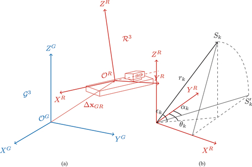
Figure 1. (a) shows the relationship of Cartesian coordinate systems: blue – the superior global coordinate system ${\mathcal{G}}^3$ (i.e. point cloud’s CS); red – the radar system ${\mathcal{R}}^3$. $\mathrm{\Delta }{\mathbf{X}}_{\mathit{GR}}$ shows the translation vector between the global and radar coordinate origins. In (b) a 3d scatterer $S_k$ is given with elevation angle ${\in }_k$ and azimuth ${\theta }_k$ which will be mapped by the radar imaging process to $\mathit{S}{{\mathit{ }}^{\mathrm{\prime }}}_{\mathit{k}}$ represented in the ${\mathcal{R}}^2$ system with range $r_k$ and cross-range ${\alpha }_k$.

2.2. Radar coordinate systems

A GB-SAR typically has an antenna unit, carrying the individual transmitting and receiving antennas, that is mechanically moved along a linear rail. With these, the range $\mathit{r}$ and the cross-range $\mathit{\alpha }$ of backscattering objects, the so-called scatterers, are sensed. By moving the antenna unit along the rail and appropriate processing of the raw data, a larger antenna is synthesized (Rödelsperger 2011). The cross-range resolution $\mathrm{\Delta \alpha }$ (expressed as half power beam width) for linear GB-SAR is given by $\mathrm{\Delta }\mathit{\alpha }=\frac{\lambda }{2\mathit{L}}$ (Caduff et al. 2015), which depends on the wavelength $\mathit{\lambda }$ of the transmitted signal and the length $\mathit{L}$ of the antenna phase centre’s trajectory, i.e. approximately the length of the rail. The range resolution $\mathrm{\Delta }\mathit{r}=\frac{c}{2\mathit{BW}}$ (Caduff et al. 2015) is depending on the signal bandwidth $\mathit{BW}$ and the speed of light. The result of a GB-SAR observation is a radar image in the 2d radar image coordinate system ${\mathcal{S}}^2$, commonly given in the form of an SLC, as shown in Figure 2a.

Figure 2. Polar and Cartesian representation of TRI observations. SLC in 2d radar image space ${\mathcal{S}}^2$ (a) and bins projected into 2d Cartesian space ${\mathcal{R}}^2$ (b). The cells in yellow share the same range index, whereas all cells in blue have the same cross-range index. The resolution cell RC(i,j) marked in green contains the amplitude and phase information encoded in complex form for a specific range/cross-range index.

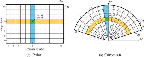
Each resolution cell (RC) contains the observed phase and amplitude with an assigned cross-range index $\mathit{i}$ and range index $\mathit{j}$, from which the polar coordinate $(\mathit{r},\mathit{\alpha })$ are computed by multiplying with their respective resolutions, $\mathit{r}=\mathit{j}\times \mathrm{\Delta }\mathit{r}$ and $\mathit{\alpha }=(\mathit{i}-\mathit{N}/2)\times \mathrm{\Delta }$. Given the aforementioned polar coordinates, the data can be projected into a 2d radar Cartesian coordinate system ${\mathcal{R}}^2$ as depicted in Figure 2b using the common polar to Cartesian conversion $x^P=\mathit{r}\times sin\mathit{\alpha }$, and $y^P=\mathit{r}\times cos\mathit{\alpha }$. It is to mention that this, in general, does not bring the radar image into an orthographic projection of the 3d space, i.e. horizontal coordinates (as it will be discussed in Section 3), although for some scenes, the resulting amplitude image may roughly resemble an orthophoto of the corresponding real-world area.

We perform georeferencing in the Cartesian space. For this, we introduce the 3d Cartesian coordinates system ${\mathcal{R}}^3$ for the radar instrument, as depicted in red in Figure 1a. The Origin ${\mathcal{O}}^R$ is set to be located in the middle of the rail. The $X^R$-axis is defined parallel to the trajectory of the antenna-phase centre during the translation of the radar sensor module along, i.e. parallel, the linear rail. The $Y^R$-axis is defined parallel to the antenna boresight. The Z-axis complements it to a right-handed Cartesian coordinate system. To solve the georeferencing problem, the relative transformation has to be established between this system and the superior global coordinate system ${\mathcal{G}}^3$, in which the point cloud is given.

3. Transformation and mapping between the systems

The common imaging radar systems that can be found in the literature are the linear GB-SAR, e.g. FastGBSAR (Placidi et al. 2015), or IBIS-FM (Farina et al. 2011) from IDS Geosystem s.r.l. and the terrestrial RAR, like the GPRI of Werner et al. (2008) from Gamma Remote Sensing AG. The mapping equations derived in this study are based on the working principle of the linear GB-SAR system and RAR and in the experimental part of this work we use GB-SAR. Adaptions for other types of systems as listed by Pieraccini and Miccinesi (2019) are left for future work.

Georeferencing requires defining bidirectional mapping equations that would allow the representation of both TRI and point cloud data in both the above-mentioned reference systems. Hence, in the following, the transformation from the 3d point cloud to the polar TRI system will be described and vice versa.

3.1. 3d point cloud to TRI: G3 → R2

The transformation from 3d rectilinear space in which the point cloud is defined (${\mathcal{G}}^3$) takes place in two steps. The first step transforms the individual points from ${\mathcal{G}}^3$ into the 3d rectilinear space of the radar system ${\mathcal{R}}^3$, which accounts for the position and orientation of the radar instrument in relation to the point cloud. The second step is the projection of the 3d points in ${\mathcal{R}}^3$ into the 2d representation ${\mathcal{R}}^2$, which accounts for the radar imaging process. With the given unique mapping, a closed-form solution can be found. The first step is given by

(1) ${\mathbf{X}}^G=\mathrm{\Delta }{\mathbf{X}}_{GR}^G+{\mathbf{C}}_R^G{\mathbf{X}}^R,$(1)

(2) ${\mathbf{C}}_R^G=\mathit{m}{\mathbf{R}}_R^G{H}_R^G,$(2)

and it consists of a translation $\mathrm{\Delta }{\mathbf{x}}_{GR}^G$, of points to the radar origin ${\mathcal{O}}^R$ and a transformation ${\mathbf{C}}_R^G$ which encompasses rotation ${\mathbf{R}}_R^G$, change of handedness ${\mathbf{H}}_R^G$ and scale $\mathit{m}$. The translation $\mathrm{\Delta }{\mathbf{x}}_{GR}^G=[T_X,T_Y,T_Z]$ is equal to the radar position in the global system ${\mathcal{G}}^3$ and the rotation matrix (with $\mathit{s}\widehat{=}sin(\cdot ),\mathit{c}\widehat{=}cos(\cdot )$) given by

(3) $\begin{array}{cc}{\mathbf{R}}_R^G& ={\mathbf{R}}_Z(\mathit{\omega }){\mathbf{R}}_Y(\mathit{\psi }){\mathbf{R}}_X(\mathit{\gamma })\\ \mathit{\hspace{0.17em}}& =\left[\begin{array}{ccc}\mathit{c}(\mathit{\omega })& -\mathit{s}(\mathit{\omega })& 0\\ \mathit{s}(\mathit{\omega })& \mathit{c}(\mathit{\omega })& 0\\ 0& 0& 1\end{array}\right]\left[\begin{array}{ccc}\mathit{c}(\mathit{\psi })& 0& \mathit{s}(\mathit{\psi })\\ 0& 1& 0\\ -\mathit{s}(\mathit{\psi })& 0& \mathit{c}(\mathit{\psi })\end{array}\right]\left[\begin{array}{ccc}1& 0& 0\\ 0& \mathit{c}(\mathit{\gamma })& -\mathit{s}(\mathit{\gamma })\\ 0& \mathit{s}(\mathit{\gamma })& \mathit{c}(\mathit{\gamma })\end{array}\right]\end{array}$(3)

describes the orientation of the radar. The handedness is predetermined and is not an outcome of the estimation process. Therefore, in most cases, ${\mathbf{H}}_R^G=\mathit{I}$, when the handedness is equal between the systems. In other cases, ${\mathbf{H}}_R^G$ has to be set to the permutation matrix to get to the right-handed system.

To get to the radar system ${\mathcal{R}}^3$, the transformation is equal to

(4) ${\mathbf{x}}_k^R=({\mathbf{C}}_R^G{)}^{-1}({\mathbf{x}}_k^G-\mathrm{\Delta }{\mathbf{x}}_{GR}^G),$(4)

where $\mathit{k}$ denotes an individual scatterer. For the second step, for each scatterer $S_k$, the range $r_k$ and cross-range ${\alpha }_k$ in the 2d radar image can be calculated from the above ${\mathbf{x}}_k^R$. The range is independent of rotation and handedness and thus equals

(5) $r_k=||{\mathbf{x}}_k^R||=(1/\mathit{m})||{\mathbf{x}}_k^G-\mathrm{\Delta }{\mathbf{x}}_{GR}^G||+\mathit{\delta r}.$(5)

For a GB-SAR system with a linear rail, the cross-range is the angle between the radar instrument’s $Y^R$ axis (as defined in section 2) and the corresponding scatterer’s position vector, i.e.:

(6) ${\alpha }_k=arcsin\left(\frac{x_k^R}{r_k}\right)+\mathit{\delta \alpha }$(6)

whereas $x_k^R$, $y_k^R$ and $z_k^R$ are the Cartesian coordinates of the scatterer $S_k$ as it can be seen in Figure 1b. The cross-range ${\alpha }_k$ will constraint within a range (e.g. for the IBIS-FM system ${\alpha }_k=\left[-{50}^{\circ },+{50}^{\circ }\right]$) determined by the limited beam width of the antenna.

For a RAR system, the azimuth is equal to

(7) ${\theta }_k=arctan\left(\frac{x_k^R}{y_k^R}\right)+\mathit{\delta \theta }.$(7)

In a preliminary study by Wieser et al. (2020), it was shown that adding additional parameters accounting for a range offset $\mathit{\delta r}$ and cross-range offset $\mathit{\delta \alpha }$, and respectively azimuth offset $\mathit{\delta \theta }$, can sometimes be required unless the instrument or the measurement configuration does not need it (like in our case in Section 6).

3.2. TRI to point cloud: R2 → G3

When facing the inverse problem we want to compute the 3d position $\left[x_k^G,y_k^G,z_k^G\right]$ from the given range $r_k$ and cross-range ${\alpha }_k$. Transforming the radar observation into 3d space is non-unique due to the under-determined equation system with two knowns ($r_k$, ${\alpha }_k$) and three unknowns ($x_k^G$, $y_k^G$, $z_k^G$). To resolve this additional information has to be introduced. For this, we first need to understand the geometrical representation of an SLC in ${\mathcal{R}}^3$. As described in the previous section, each resolution cell (RC) is defined by a range and cross-range in ${\mathcal{R}}^2$. The range index, respectively. the range of a RC, defines in ${\mathcal{R}}^3$ a spherical shell with inner radius $((\mathit{j}-1/2)\cdot \mathrm{\Delta r})$ and outer radius $((\mathit{j}+1/2)\cdot \mathrm{\Delta r})$, centred at the origin ${\mathcal{O}}^R$, as depicted in yellow in Figure 3a. All scatterers within this volume have the same range index, as shown in Figure 2. The cross-range $\mathit{\alpha }$ is the complementing angle to ${90}^{\circ }$ from the $Y^R$-axis to the position vector of the scatterer in the $X^R{Y}^R$-Plane. As linear GB-SAR measurements are insensitive to the rotation of the instrument around the $X^R$-axis, all the scatterers within the cone defined by $\mathit{\alpha }=(\mathit{i}\pm 1/2)\times \mathrm{\Delta \alpha }$, with the vertex at ${\mathcal{O}}^R$ as depicted in Figure 3b, have the same cross-range index. Therefore, ${\mathbf{R}}_X$ is undetermined (but also irrelevant) for linear GB-SAR, i.e. it cannot be estimated from GB-SAR data. In such a case, ${\mathbf{R}}_X$ can be fixed by definition, e.g. setting ${\mathbf{R}}_X=\mathit{I}$.

Figure 3. Visualization of the range and cross-range parameters as sensed in 3d by a linear GB-SAR. The figure directly relates to the 2d representation in Figure 2. Figure 3a depicts the volume in which all scatterers get the same range index. Figure 3b shows accordingly the region of the same cross-range index. Figure 3c depicts then the intersection of the former two shapes and represents the volume in which all scatterers contribute to the same image pixel.

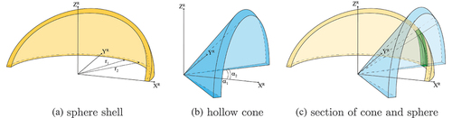
Now, all the scatterers within the volumetric intersection as depicted in green in Figure 3c are mapped to the same pixel of an SLC. It is important to mention that the schematic visualization does not fully represent the real volume as the cone and sphere are limited by the antenna gain pattern in reality.

The process can be inverted by searching for the positions in ${\mathcal{G}}^3$ which the radar imaging maps to a specific range and cross-range. For this, a 3d representation of the monitored surfaces is needed such that the elevation angle $\in$, as depicted in Figure 1b, can be extracted, which is needed for the calculation of $y_k^R$ and $z_k^R$. The search for the optimal assignment for each individual point is complex and will not be studied in this work. A solution proposal is given in Rebmeister et al. (2022). In this study, we use a simple approach and assign the SLC pixel to the point cloud based on a nearest-neighbour search.

The mapping function introduced here for linear GB-SAR differs from the ones usually found in the literature, e.g. by Monserrat (2012), especially regarding how the cross-range information is mapped into 3d. The assessment of this impact will follow in Section 4.2. An alternative worth investigating in the future is simultaneous computation and georeferencing of SLCs, for example based on the range Doppler model (Nedelcu and Brisco 2018). However, such investigations are out of the scope of this work.

4. Corresponding features and feature mapping

To solve for the parameters of the transformation equations presented in Equation. 4(4) ${\mathbf{x}}_k^R=({\mathbf{C}}_R^G{)}^{-1}({\mathbf{x}}_k^G-\mathrm{\Delta }{\mathbf{x}}_{GR}^G),$(4) , we need data points from both datasets representing the same scatterer in the real world. This task is challenging because no direct feature relations are available due to the different characteristics (e.g. wavelength and resolution) of the technologies used to obtain the radar image and the 3d model. The solutions presented in the literature typically rely on in situ targets (see Section 1), resulting in high signal backscatter which can be detected in the radar image, identified in the point cloud and thus used to match both datasets. All presented studies rely on visual identification of these high-amplitude scatterers (e.g. artificial corner reflectors or highly reflective metal objects) based on expert knowledge or on a highly accurate survey of the instrument pose to be able to directly infer the transformation parameters. But all these approaches either do not allow for a fully automatic end-to-end process due to the need for manual input or enter and alter physically the region of interest, which can be costly, cumbersome, dangerous or sometimes just not possible. To tackle these challenges and enable an automatic georeferencing workflow, we developed an approach for building the correspondences between the detected high-amplitude scatterers in TRI data and the natural features found in point clouds. Those are features in the data corresponding to particular natural formations with the possibility of their localization and identification. Defining and matching these features will be elaborated on in the following sections.

4.1. Feature definition

For radar datasets, we use radar pixels with high amplitude values as features, following the aforementioned established approaches in the literature. For point clouds, we need to compute proxies of these features, corresponding to the pixels of high amplitudes, solely from data that are inherently part of a point cloud. In search of the appropriate feature, we tested overall 24 geometrical features that can be derived from local point cloud geometry, of which 22 are implemented in the open-source software CloudCompare (CloudCompare 2022). The short description can be found in the software wiki (CloudCompare 2023), while the more detailed description for most features can be found in Hackel, Wegner, and Schindler (2016) and Douros and Buxton (2002). Additionally, we computed the hillshade (Burrough and McDonnell 1998) and angle of incidence (AOI). We also tested a multitude of their linear and nonlinear combinations. These were then visually inspected to find features or feature combinations that provide a good distribution of extreme values that coincide with the high-amplitude radar pixels. Additionally, as the feature values are calculated per individual point in the point cloud and depend on the distribution of neighbouring points, we tested different neighbourhood sizes, varying them around the radar pixel’s resolution. In the end, the simple AOI proved to be the best candidate for use. The AOI is equal to the angle between the vector of a point cloud point position relative to the approximate position of the TRI instrument and the surface normal vector of this point. With increasing incidence angle, the amplitude of the backscattered signal is expected to decrease. Conversely, areas with incidence angles close to $0^{\circ }$ are expected to correspond to direct signal reflection back to the instrument and thus show the highest amplitude values in the radar image. This assumption is also supported by the model choice of Rebmeister et al. (2022) used for linking the incidence angle and the backscattered intensity of these points for refining the position of the scatterer within an RC. The normal vectors are computed by fitting a local plane through a selected set of points in the neighbourhood of each point in the point cloud. The neighbourhood radius $r_f$ should be chosen similar to the surface area corresponding to the RCs of the radar image (i.e. similar to the highest achievable resolution with TRI).

Once these approximate corresponding features have been found, the main remaining challenge for georeferencing is the absence of an unambiguous correspondence between discrete feature pairs – the salient locations with the high amplitude (radar) and the low incidence angle (point cloud). For visualization of the discrepancies, we used the features from the dataset of the later experimental validation (Sec. 6) and projected them onto the point cloud. In Figures 4(a, b), a large difference in the level of detail is visible. The higher spatial resolution of the point cloud AOI feature can reveal much finer details in comparison to the amplitude feature radar dataset. For the extreme values (high amplitude, low incidence angle), a good qualitative agreement can be observed, e.g. along the edge depicted in Figure 5a. From this visualization, it can also be seen that the agreement is ambiguous, which means that multiple RCs showing high amplitude are only approximately corresponding to multiple points having a low AOI (i.e. not a one-to-one match considering their shape, size and distribution). Hence, the approaches relying on (manually identified) individual scatterers with direct correspondence cannot be readily applied. Therefore, we propose the use of the kernel correlation algorithm, as established by Tsin and Kanade (2004) as summarized in the following section.

Figure 4. Features used as input for the georeferencing. (a) shows the amplitude information projected on a point cloud, using the approach presented in 3.2. (b) shows the computed incidence angle of the point cloud dataset based on the approximately known TRI location. The regions for the detailed views as depicted in Figure 5 are marked with the red boxes.

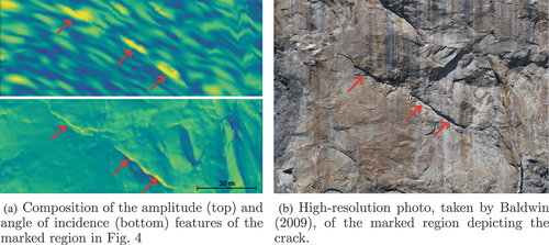
Figure 5. Detailed view (a) of the selected region shows a crack which is visually represented by high amplitude and angle of incidence features. In fig. (b) the crack is clearly visible in the centre of the photo.

4.2. Feature matching

Kernel Correlation (KC) was originally proposed as a method for image registration. The goal of correlation-based algorithms is to minimize the difference between the corresponding pixel values (appearance information) of two images by applying transformations to one of the images. The approach can also be applied to registering sparsely and irregularly sampled point sets by transforming them into image representations by generating 2d density images. This is achieved by separating the space in regular grids and mapping the number or density of points per grid cell using a mapping kernel. Once these density images are generated, the optimal set of transformation parameters is found by maximizing the correlation of the density images (Kernel Correlation, KC). The density $\mathit{P}(\mathbf{x})$ at a point $\mathbf{x}$ in point set $\mathcal{X}$ (consisting of $N_P$ points) is approximated by the Kernel density estimate (KDE):

(8) $\mathit{P}(\mathit{x})=\sum _{\mathit{i}=1}^N\mathit{K}(\mathbf{x},{\mathbf{x}}_{\mathbf{i}})/N_P,$(8)

where $\mathit{K}$ is the chosen kernel function whose values depend on the distance between $\mathbf{x}$ and ${\mathbf{x}}_{\mathbf{i}}$. When using this for the point set registration, the rigid body transformation between these sets is iteratively updated, until the optimal transformation parameters $\mathit{\theta }$ are found as those maximizing the cost function. We used the discrete version of the cost function as given in Tsin and Kanade (2004),

(9) $\mathcal{C}\mathcal{O}\mathcal{S}\mathcal{T}(X_S,X_M,\mathit{\theta })=-\sum _x{P}_S(\mathbf{x})P_M(\mathbf{x},\mathit{\theta }),$(9)

where ${\mathcal{P}}_S(\mathbf{x})$ is the discrete KDE of the fixed point set $X_S$ at grid point $\mathbf{x}$ and ${\mathcal{P}}_M(\mathbf{x},\mathit{\theta })$ is the KDE of the transformed point set $\mathit{X}{{\mathit{ }}^{\mathrm{\prime }}}_{\mathit{M}}=\mathit{T}({\mathbf{x}}_{\mathbf{M}},\mathit{\theta })$, with $\mathit{T}$ being transformation. In our case, the $X_S$ represents the radar data points and $X_M$ the point cloud points. The KDE also allows us to correlate datasets with different spatial resolutions due to the fixed kernel size and the normalization ($N_P$), which is relevant for our use case as the TRI and TLS observations are different in that regard. The transformation $\mathit{T}$ is given by Equations. 5(5) $r_k=||{\mathbf{x}}_k^R||=(1/\mathit{m})||{\mathbf{x}}_k^G-\mathrm{\Delta }{\mathbf{x}}_{GR}^G||+\mathit{\delta r}.$(5) and 6(6) ${\alpha }_k=arcsin\left(\frac{x_k^R}{r_k}\right)+\mathit{\delta \alpha }$(6) in our case.

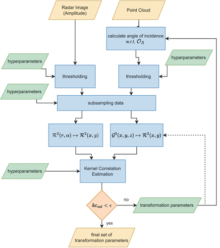
5. Proposed workflow

The previously introduced mapping equations, the computations of loosely corresponding features and the search for the optimal set of transformation parameters are now combined into an automatic georeferencing workflow for mapping the radar images onto the point cloud. All the steps of the proposed workflow are consolidated in Figure 6. In our workflow, we first filter the datasets by individual heuristically chosen thresholds to isolate the regions with indicative feature values, i.e. high radar amplitude and low AOI. In our case, we kept the data points with radar amplitude $>$ 4 (corresponds roughly to the 3% SLC bins with highest amplitudes), resulting in $N_{\mathit{R},\mathit{F}}$ filtered points, and the point cloud data points with AOI $<$ 15 degrees (2% with lowest AOI), which equals to $N_{\mathit{G},\mathit{F}}$ points. In the next step, both datasets get subsampled to increase the computation efficiency, resulting in sparse datasets with equal amounts of points. In our case, the point cloud dataset has more points than the radar image, and therefore, we chose the subsampling rate ${\nu }_R$ (herein 1%) for the radar image and then subsampled the point cloud to have the same number of points in both datasets ($N_{\mathit{R},\mathit{S}}={\nu }_R\times N_{\mathit{R},\mathit{F}}$, resulting in 1% of radar points and an equal number of point cloud points $N_{\mathit{G},\mathit{S}}=N_{\mathit{R},\mathit{S}}$). Then, the 3d point cloud gets projected into ${\mathcal{R}}^2$ using Equations. 5(5) $r_k=||{\mathbf{x}}_k^R||=(1/\mathit{m})||{\mathbf{x}}_k^G-\mathrm{\Delta }{\mathbf{x}}_{GR}^G||+\mathit{\delta r}.$(5) and 6(6) ${\alpha }_k=arcsin\left(\frac{x_k^R}{r_k}\right)+\mathit{\delta \alpha }$(6) using appropriately chosen initial values of all transformation and mapping parameters, i.e. the unknowns to be determined as part of georeferencing. We will investigate in Section 6, how close to the real values these initial values have to be.

Figure 6. Flow chart of the proposed algorithm using a radar image and a point cloud as input and providing a set of optimal transformation parameters as output.

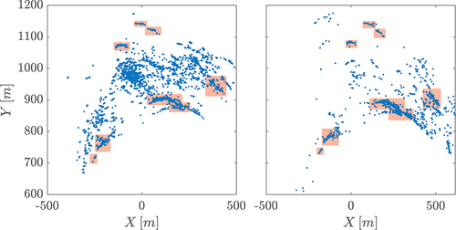
For georeferencing, only the location of the filtered and subsampled points is further used, not the values of radar amplitude or AOI. An example of the resulting datasets is shown in Figure 7.

Figure 7. Example of a set of subsampled points used to compute the kernel density estimates (KDE) for the kernel correlation process. The left figure shows the amplitude filtered points (amplitude $>$ 4) of the radar data and on the right the filtered points (AOI$<$15 deg) of the point cloud data. The red highlighted areas show visually identified corresponding features.

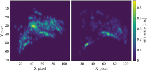
These reduced datasets are then used as input for the KC algorithm. There, the KDE is computed. For this, a grid with a given kernel size is spanned and the kernel density with a Gaussian kernel is computed. For the latter data processing in this paper, we chose a pixel size (grid size) of g = 10 m for the kernel density images and a Gaussian kernel with shape parameter h = 10 m. An example of the density images is shown in Figure 8. Finally, the transformation parameters are estimated by maximizing the correlation of the KD images according to Equation. 9.(9) $\mathcal{C}\mathcal{O}\mathcal{S}\mathcal{T}(X_S,X_M,\mathit{\theta })=-\sum _x{P}_S(\mathbf{x})P_M(\mathbf{x},\mathit{\theta }),$(9) We chose to solve the optimization problem using the Nelder-Mead simplex method by Lagarias et al. (1998) which generates a new set of (tentative) transformation parameters until the convergence criterion is met $\mathit{k}{c}_{\mathit{val}}<\in$, with the correlation value $\mathit{k}{c}_{\mathit{val}}$ (current evaluation of cost function) and the convergence limit $\in$. After each estimation, the transformation parameters have to be applied to the initial dataset and the AOI has to be recomputed, following the straight return path in Figure 6. If the estimated transformation has a negligible impact on the AOI, the dotted path in Figure 6 can be chosen.

Figure 8. Example of the computed normalized kernel density image (left: radar data, right: point cloud data), estimated from the subsampled points (as depicted in Figure 7) for the kernel correlation registration.

6. Experiments & results

In the previous sections, we tackled several challenges in order to provide a full end-to-end georeferencing approach for radar images. In the following, we assess the individual parts of our proposed approach using a real-world dataset for which this type of transformation application is applicable.

6.1. Dataset and Preprocessing

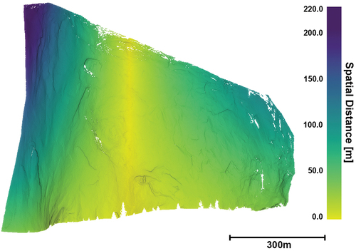
Our study area, El Capitan cliff, is located approximately 250 km east of San Francisco, California (USA) in Yosemite National Park. El Capitan is one of the world-famous granitic cliffs, exposed in Yosemite Valley, a 1000-m-deep, glacially sculpted valley within the central Sierra Nevada mountain range. We acquired GB-SAR data of the southeast face of El Capitan using an IBIS-FL interferometric radar positioned at 950 m mean range from the cliff. The southeast face of El Capitan is approximately 520,000 m² in area with a near-vertical relief. Radar data were collected continuously at 2-min intervals for a period of approximately 6 months beginning in October 2019. The SLC used in our evaluation is an averaged aggregate from a few hundred SLCs with the goal of reducing the noise.

For the point cloud, ground-based (terrestrial) LiDAR data were collected as part of a separate project by the University of Lausanne (Switzerland) in 2013 using an Optech LR scanner. The scanner was set up at a range of 1000 m from the cliff and provided full coverage of the cliff’s face with a mean point spacing of 25 cm. The LiDAR data were transformed into a right-handed Cartesian coordinate system (${\mathcal{G}}^3$) with its origin approximately at the centre of the radar instrument, the $X^G$ axis approximately parallel to the instrument’s rail, and the $Z^G$ axis approximately vertical. They were filtered to a mean 50 cm point spacing. The spatial extent of the area monitored within our study site is comparable to the related documented application cases of TRI (mostly focusing on monitoring landslides, mines and other geologically active regions), as, e.g. described by Pieraccini and Miccinesi (2019).

6.2. Assessment of mapping equations

Until now, for most georeferencing tasks, the simple 3d-georeferencing algorithm as presented, e.g. by Monserrat (2012) is used. There, for each point of the point cloud (or DEM), the respective range $\mathit{r}$ and azimuth $\mathit{\alpha }$ are computed. Then, the respective radar pixel coordinates with the range index $\mathit{j}$ and cross-range index $\mathit{i}$ are derived by division of the range and azimuth by the range and cross-range resolution’s $\mathrm{\Delta \alpha }$ and $\mathrm{\Delta r}$. Then, for each point, the radar information is assigned from the closest radar pixel to the computed coordinates ($\mathit{i}$,$\mathit{j}$), or the information is interpolated from the neighbouring pixels. This simplified mapping is straightforward to compute, but it does not fully represent the imaging process of a linear GB-SAR because the difference between cross-range and azimuth is not taken into account. We have shown in Sec. 3 and Figure 1b that the sensed cross-range $\mathit{\alpha }$ for linear GB-SAR should not be treated as the azimuth $\mathit{\theta }$. The difference $\mathit{\delta }$ between the sensed cross-range $\mathit{\alpha }$ and the azimuth $\mathit{\theta }$ can be expressed as:

(10) $\begin{array}{cc}\mathit{\delta }& =\mathit{\theta }-\mathit{\alpha }\\ \mathit{\hspace{0.17em}}& =\mathit{\theta }-arctan\frac{sin\mathit{\theta }}{\sqrt{{tan}^2\in +{cos}^2\mathit{\theta }}}\end{array}$(10)

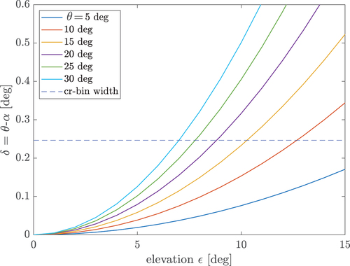
So, for low elevation angles ($\in \approx 0$), cross-range and azimuth are indeed almost equal. However, for elevation angles larger than a few degrees, the difference between $\mathit{\alpha }$ and $\mathit{\theta }$ may be relevant. In Figure 9, $\mathit{\delta }$ is plotted as a function of the elevation angle, $\in$ for scatterers with different azimuth $\mathit{\theta }$ ($5^{\circ }-{30}^{\circ }$). For comparison, the cross-range resolution $\mathrm{\Delta \alpha }={0.25}^{\circ }$ for the IBIS-FL system is depicted as a dashed blue line. For observation of scatterers with a moderate elevation up to $5^{\circ }$, the difference is below the cross-range bin width, which can be considered negligible. But if the difference is larger than $\mathrm{\Delta \alpha }$, cell migration occurs, which means that the 3d surface element will be assigned to the wrong SLC bin. This effect is amplified with increased azimuth $\mathit{\theta }$, so with larger angular distance from the antenna boresight. It is worth noting that $\mathit{\delta }$ is independent of range $\mathit{r}$.

Figure 9. Difference between azimuth $\mathit{\theta }$ and cross-range $\mathit{\alpha }$ as the function of elevation angle $\in$ for different $\mathit{\theta }$.

In Figure 10, the spatial error due to assuming cross-range and azimuth to be equal for a linear GB-SAR is shown for the scatterers in our study site. The largest errors occur at locations with high elevation and far from the antenna boresight. When applying the correct mapping function as per Equation. 6(6) ${\alpha }_k=arcsin\left(\frac{x_k^R}{r_k}\right)+\mathit{\delta \alpha }$(6) , the expected improvement for our study site is more than 200 m for the extreme locations on the cliff. A more detailed evaluation is followed up in Section 6.3 (i).

Figure 10. Impact of the difference between the azimuth $\mathit{\theta }$ and cross-range $\mathit{\alpha }$ on our study area of El Capitan.

6.3. Assessment of georeferencing precision

In this section, we assess the quality of georeferencing based on the proposed workflow, as introduced in Section 5. The analysis is separated into four parts:

1. empirical analysis of mapping errors based on visual scoring,

2. quality assessment of the estimated radar pose parameters in the parameter space,

3. quality assessment of the estimated radar pose parameters in 3d coordinate space and

4. empirical analysis of the admissible deviation of the initial values.

Visual scoring

To empirically assess the impact of choosing a different mapping function, we propose an evaluation based on visual scoring. For that, we visually identify corresponding feature patches in the AOI map and in the projected amplitude map (e.g. in Figure 4). This is similar to the georeferencing approaches based on manually detected features commonly used in the reviewed literature (Section 1). Once correspondences are visually defined, the spatial distance between the visually estimated centroids of corresponding feature patches is measured. This procedure has limited precision, as there is no one-to-one match considering the shape, size and distribution of feature patches. Hence, the mapping precision derived this way should be taken with caution regarding the absolute values presented, as we are introducing additional errors during visual centroid identification. This also means that the achieved mapping precision is potentially higher than the presented one as the implemented georeferencing workflow circumvents this bottleneck by using kernel correlations. Despite these limitations, this evaluation procedure can still deliver a good understanding of relative mapping improvements introduced by the proposed workflow. We note here that we relied on manual identification of natural features as no data-driven alternative is presented in the literature and installing dedicated targets (e.g. corner cube reflectors) was not possible in the area under investigation.

For clarity, in Figure 11, we show an example for three identified feature pairs in regions A, B and C for the mapping of radar amplitudes on the point cloud with (1) the standard equations and only approximately known radar pose, (2) our modified mapping function and approximately known radar pose and (3) our modified mapping function and the refined radar pose using the proposed workflow. With the black arrow, we indicate the distance between the visually (approximately) estimated centroids. The results of all corresponding pairs which we could identify are summarized in the boxplots in Figure 12. Additionally, each individual distance is plotted as an individual data point.

Figure 11. Comparison of the spatial distance of the visually identified feature correspondences of radar amplitude and angle of incidence. Three regions A, B and C are depicted with (1) the standard mapping and only approximately known radar pose, (2) the mapping according to Equation (6) and approximately known radar pose and (3) the mapping according to Equation (6) and the refined radar pose obtained from the proposed workflow. The black arrow shows an example of a patch pair used for visual scoring.

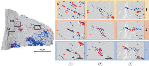
Figure 12. Boxplot of 3d distances of visually identified feature correspondences of radar amplitude and angle of incidence patches for the standard mapping equation. ($\mathit{med}=41.9\mathit{m},\mathit{MAD}=9.2\mathit{m}$), our new mapping equation ($\mathit{med}=9.5\mathit{m},\mathit{MAD}=2.1\mathit{m}$), and the result after georeferencing with our workflow ($\mathit{med}=4.3\mathit{m},\mathit{MAD}=1.0\mathit{m}$).

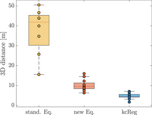
It can be seen that the application of the correct mapping function instead of the standard one leads to substantial improvements. The mean spatial distance of the patches could be reduced from 41.9 m (for the standard mapping) to 9.5 m (using Equation. 6(6) ${\alpha }_k=arcsin\left(\frac{x_k^R}{r_k}\right)+\mathit{\delta \alpha }$(6) ), corresponding to a reduction in mapping error by more than 75%, see also Figure 12. Additionally, the median absolute deviation (MAD) of distance values is also reduced from 9.2 m to 2.1 m, showing a notable reduction in variability of systematic mapping distortions depending on different elevation and azimuth angles (as demonstrated in Figure 9). The largest improvement can be seen for features with higher elevations, which is in line with the impact of the elevation angle according to Eq. 10(10) $\begin{array}{cc}\mathit{\delta }& =\mathit{\theta }-\mathit{\alpha }\\ \mathit{\hspace{0.17em}}& =\mathit{\theta }-arctan\frac{sin\mathit{\theta }}{\sqrt{{tan}^2\in +{cos}^2\mathit{\theta }}}\end{array}$(10) and Figures 9 and 10.

By introducing the proposed workflow, the median spatial distance between the visually identified feature patch centroids could be additionally reduced from 9.5 m (achieved by using the modified mapping approach) to 4.3 m, further halving the mapping error. Alongside this, the MAD could be reduced to 1.0 m (again halving the previously reported value). The finally achieved mapping errors are approximately on the level of the resolution of the projected radar pixel on the point cloud (approx. 2–6 m) for the dataset under investigation. Hence, our empirical analysis indicates that the mapping error of the proposed approach is bound to and comparable to the realized radar image resolution.

Parameter quality assessment in parameter domain

To provide some quality indicators, we analysed the precision and correlations of the radar pose parameters estimated by the proposed workflow. The assessment is done similarly to the bootstrapping approach proposed by Efron (1979) and Neuner et al. (2014). Using this approach, the estimation is repeated n times, each time drawing the initial values (approximate radar poses) from a uniform distribution within the chosen boundary. This is introduced as we also want to expose if any weakly observable parameters might be biased by the initial values given to the used Nelder-Mead simplex method. Additionally, as described in Section 5, in each estimation run, only 1% of the data points are randomly drawn from the data, again to reduce the chance of repeated convergence to some local minima. After the estimation process, the distribution of the estimated parameter is evaluated.

First, before a more detailed parameter evaluation, we checked for the observability and convergence of all translation and rotation parameters. For each parameter individually, the initial value is drawn 1000 times from the uniform distribution between ±5 m for the translation or ±5 deg for the rotation, centred at 0, while all other parameters are set to 0. The adequate convergence of a parameter is confirmed, if the estimated values are normally distributed around its mean and have a standard deviation being a fraction of the sampling interval.

The results are presented in Table 1. It can be observed that all parameters besides one converge within the given sampling interval, confirming their observability. Only the rotation around the $X^R$-axis cannot be estimated, which was already discussed in a relation to the functional principle of the GB-SAR systems in Section 2. We included ${\mathbf{R}}_X$ in this analysis until here only for demonstration purposes. For the remainder, we set ${\mathbf{R}}_X=\mathit{I}$ and did not estimate the corresponding rotation.

Table 1. Summarized results of the convergence assessments. The first and second rows show the result of the assessment per-parameter basis; the first depicts the result of the 6-parameter model including rx, and the second the 5-parameter model without rx. The third line shows the result where all parameters were initialized simultaneously.

Tx (m)		Ty (m)		Tz (m)		Rx (°)		Ry (°)		Rz (°)
mean	$\mathit{\sigma }$	mean	$\mathit{\sigma }$	mean	$\mathit{\sigma }$	mean	$\mathit{\sigma }$	mean	$\mathit{\sigma }$	mean	$\mathit{\sigma }$
2.1	1.1	−0.7	0.3	−1.7	0.6	0.5	10.5	−2.0	0.4	−0.8	0.2
2.1	1.2	−0.7	0.3	−1.7	0.6	-	-	−2.0	0.4	−0.8	0.2
2.0	1.5	−0.1	1.3	−1.4	2.7	-	-	−1.9	0.4	−0.6	0.3

For the precision and correlation analysis, the same configuration is used as in the preceding assessment, except that now all initial parameter values are randomly drawn simultaneously. The results of the analysis can be seen in Table 1 (last row) and Figure 13. The precision (standard deviations $\mathit{\sigma }$ in Table 1) of the estimated parameters is within 1.3 to 2.7 m for the translations and 0.2 to 0.4 deg. for the rotations. The uncertainties in translations can be directly transferred to the mapping uncertainty. The rotation uncertainties affect the mapping proportionally to the distance; they would correspond to approximately 7.1 m ($\mathit{Ry}$) and 4.7 m ($\mathit{Rz}$) for our dataset (approx. 1 km distance). These values are close to the mapping uncertainty observed by visual scoring in the previous analysis, but if accumulated somewhat larger. This can be explained by the following correlation analysis.

Figure 13. Overview of the correlation between all estimated parameters (Ry, Rz, Tx, Ty, Tz). For each parameter pair, the scatter plot and the Pearson correlation coefficient are given and on the main diagonal, the distribution of each parameter as a histogram is shown. The axis is in the unit of the respective parameter, metres for the translation and degrees for the rotation.

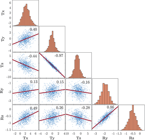
The diagonal of Figure 13 shows the distribution of the estimated parameters. The mean values and empirical standard deviations of these distributions are the values reported in the last row of Table 1. It is observable that all parameters show approximately normal distribution, giving a strong indication that the presented standard deviation is a reasonable choice for the precision metrics. The implemented workflow could thus likely be further improved by averaging multiple runs of the algorithm (each based on a randomly sampled subset of data, as above) or by increasing the size of the used subset. However, an investigation of this is left for a future, more comprehensive, study of georeferencing quality which takes the impact of various geometrical configurations (different distances, ranges and spatial distributions of features) as well as the correlations into account.

On the off-diagonal elements of Figure 13, the scatter plots of parameter pairs are shown and the Pearson correlation coefficients are given. It can be seen that a strong correlation is present between Ty and Tz (−0.97) and Rz and Ry (0.86). Also, a few other parameter pairs are correlated considerably (e.g. Rz and Tx). These high correlations indicate, on the one hand, that the geometric configuration (extent of the field of view (FoV) and the distribution of the features within FoV and in depth) is not suitable for estimating all these parameters well. Namely, all the features are distributed in a nearly planar region with a FoV extending 75° x 40° horizontally and vertically, which limits the decoupling of individual transformation parameters. However, these observed high correlations have no detrimental effect on the mapping quality, at least in this study case, as parameters are mutually compensating for each other's effects. For monitored regions with more complex geometry and larger spatial extent (wider FoV and larger depth differences), it would be worth investigating if these high correlations persist. If they persist, using alternative parameterization of the transformation equations could be beneficial, e.g. substituting Euler angle representation with quaternions or Rodrigues’ rotation. However, such an investigation is out of the scope of this work. Due to the correlations, the precision estimates presented above are not fully indicative of the georeferencing precision when studied individually. A better indicator of the georeferencing quality is provided by forward modelling the impact of the different sets of parameter values on the mapping location of individual radar bins in the 3d space, which is presented in the following analysis.

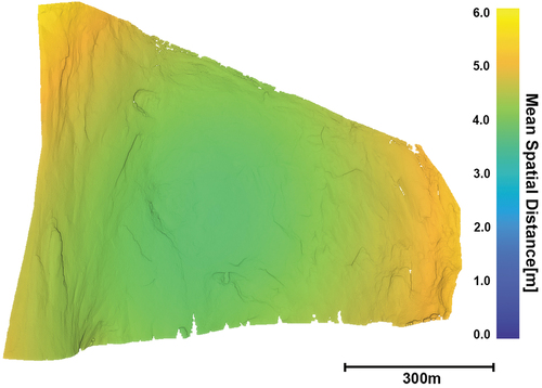
Parameter quality assessment in 3d space

We now analyse the mapping uncertainty in the 3d coordinate domain by applying the estimated sets of parameters and quantifying for each bin of the radar image the variability of the calculated locations in 3d space. This is done by transforming all points by the previously obtained 1000 estimated sets of transformation parameters, which gives for each point 1000 different positions. As a measure of the uncertainty (distribution) for each point, the mean absolute deviation to the mean position is computed. This shows the effect of the transformation for all the points, depending on their relative position to the radar sensor. As can be seen in Figure 14, the average mean deviation in the middle of the wall is approximately 4 m and increases towards the edge up to 6 m. These values correspond well to the values observed by visual scoring (median 3d distance of KcReg = 4.3 m; Figure 12) and are expectedly smallest in the centre of gravity of all feature points used to estimate the parameters. Hence, this analysis indicates that the proposed approach achieves a mapping uncertainty approximately equal to the median size (4.8 m) of the projected SLC pixel in Euclidean space. The latter is calculated as the median spatial extent of point cloud points corresponding to individual pixels along the largest PCA component.

Figure 14. Average mean deviation of 1000 estimated sets of transformation parameters estimated using the modified mapping function and the refined radar pose using the proposed workflow.

Allowable uncertainty of initial parameter values

In the previous assessment, the two datasets (TRI image and TLS point cloud) were initially aligned with errors lower than 2 m and 2 deg, based on the field observations. The refined values of the transformation parameters were estimated based on 1000 runs with randomly picked subsets of the data and randomly varied initial values (see Table 1, last row).

In this analysis, we investigate how much the initial values can differ from the true solution until the optimization does not converge towards that true solution anymore. This gives an indication of how accurately the initial transformation parameters have to be known (e.g. from field measurements). For this, the previous analysis is adapted so that the initial values are drawn from a normal distribution with increasing standard deviation (1 $\mathit{\sigma }$) from 0.5 up to 20 m for the translation parameters and from 0.2 deg to 10 deg for the rotation parameters. To assess the convergence, the mean absolute error (MAE) of the mapping is computed (analogously to the analysis visualized in Figure 14) from 1000 realizations for each of the abovementioned standard deviation pairs.

As a result, the summary of the computed MAEs is depicted in Figure 15, where each pixel represents the MAE for each translation and rotation pair. The results show that even for substantial standard deviations of the initial parameter values, the proposed algorithm converges towards the true parameter values, resulting in a small mapping error. If the initial values have a too large standard deviation, the algorithm sometimes converges to local minima, which increases the MAE and lowers the precision of the mapping.

Figure 15. Mean absolute mapping error of the estimated parameters with increasing standard deviations (1 $\mathit{\sigma }$) of the initial values for the translation (${\sigma }_{\mathit{Translation}}$) and the rotation (${\sigma }_{\mathit{Rotation}}$), with respect to mapping using the true transformation parameter.

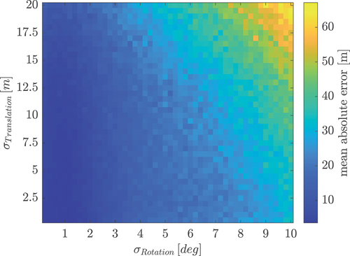
For the investigated dataset, we can observe the convergence at approximately 2 deg for the rotations and 13 m for the translations, resulting in mapping errors <5 m. These exact values are dataset dependent, and some variation is expected with changes in a measurement configuration. However, they demonstrate that accurate and costly geodetic surveys of radar pose as used in some of the reviewed works (see Section 1) can be drastically relaxed. Only an approximate instrument pose is required, e.g. realized with a low-cost GNSS receiver, compass and spirit level, and they can be successfully refined with the algorithm proposed herein to achieve metre-level precise georeferencing of the radar data. To the authors’ knowledge, this is the first algorithm that achieves this task automatically, without the need for manual feature identification.

7. Conclusion

This paper proposes an automatic approach for precise georeferencing of terrestrial radar images relative to a point cloud. The proposed approach works by identifying approximately corresponding natural features in radar and point cloud datasets (high radar amplitudes vs. nearly perpendicular angles of incidence in a point cloud) and solves for the radar pose relative (3d position and orientation) to the point cloud using the kernel correlation algorithm. Additionally, we introduced the correct mapping function representing the radar imaging process for a linear GB-SAR system where the difference between cross-range and azimuth is not negligible if the monitored area includes elevations more than a few degrees from the horizon.

We assessed the proposed workflow on a real-world dataset from the 1000-m high vertical rockface of El Capitan in Yosemite National Park, USA, and we demonstrated a mapping precision of better than 5 metres. Based on the current experiments, the success of the approach can only be expected for comparable spatial extents, which are commonly encountered in geomonitoring applications. The generalizability of the approach on monitoring the regions of larger spatial extents that require extended FoV (e.g. monitoring of open-pit mines) is still to be investigated. Moreover, the presented approach to georeferencing does not require the costly and inefficient manual feature selection and matching, which are still commonly used in the literature. Additionally, we showed that the initial alignment accuracy of the radar instrument and point cloud can be eased by 13 m for the translation and 2 deg for the rotation, significantly reducing the necessary in-field measurement efforts.

The presented assessment is so far bound to a specific dataset. Hence, although the derived values are indicative of the workflow’s performance, they are not fully generalizable. A future investigation will be necessary to assess the workflow performance in the areas with suboptimal (less reflective) surfaces, which can be encountered within landslides and vegetated areas. We aim at a more comprehensive performance assessment on different study sites paired with ground truth observations. Additionally, there are possibilities to further enhance the georeferencing approach. For example, data-driven tuning of the hyperparameters like grid size or kernel size would be beneficial for fully autonomous data processing. Finally, once a larger set of different measurement scenarios with ground truth data is available, it may be worth studying whether additional geometrical and radiometric features would support the parameter estimation. Finally, as a further development in another direction, it would be interesting to investigate if the proposed approach could be extended towards the related approaches based on the ‘Radar-Doppler geo-positioning model’, as the ones described, e.g. in Frey et al. (2012) and Xue et al. (2017) for satellite-based SAR observations. Such approaches rely on simulating entire SAR images based on DEMs and use them in an image correlation approach for geo-positioning of corresponding radar observations. Such further development would add additional complexity due to necessity of generating synthetic TRI images with sufficient fidelity and would likely require development of more complex backscattering models based on topography and system parameters. If tackling these challenges is feasible and if such additional complexity would be turned out to be beneficial for georeferencing are open questions.

Acknowledgements

“We thank Geopraevent and IDS GeoRadar for their cooperation and assistance with the collection of the TRI data used for the validation and experimental evaluation of the proposed algorithm. We acknowledge B. Matasci and M. Jaboyedoff at the University of Lausanne, Switzerland, and S. Corbett at the U.S. Geological Survey (USGS) for the collection of laser scanning data of the El Capitan rock face and Charles Miles (USGS) for providing review comments. Finally, we thank G. Stock and the ranger staff at Yosemite National Park for their assistance with field logistics during the time that the datasets were collected. Any use of trade, firm, or product names is for descriptive purposes only and does not imply endorsement by the U.S. Government

Disclosure statement

No potential conflict of interest was reported by the author(s).

Data availability statement

The data that support the findings of this study are available from the corresponding author, L. Schmid, upon reasonable request.

Correction Statement

This article has been corrected with minor changes. These changes do not impact the academic content of the article.

References

- Alba, M., G. Bernardini, P. R. Alberto Giussani, F. Roncoroni, M. Scaioni, P. Valgoi, K. Zhang, et al. 2008. “Measurement of Dam Deformations by Terrestrial Interferometric Techniques.” Int Arch Photogramm Remote Sens Spat Inf Sci 37 (B1): 133–139.
- Baldwin, J. 2009. “Yosemite’s el capitan.” Jun. http://gigapan.com/gigapans/26923.
- Burrough, P. A., and R. A. McDonnell. 1998. Principles of Geographical Information systems. Spatial Information Systems and Geostatistics. Oxford: Oxford University Press.
- Caduff, R., and D. Rieke-Zapp. 2014. “Registration and Visualisation of Deformation Maps from Terrestrial Radar Interferometry Using Photogrammetry and Structure from Motion.” Photogrammetric Record 29 (146): 167–186. https://doi.org/10.1111/phor.12058.
- Caduff, R., F. Schlunegger, A. Kos, and A. Wiesmann. 2015. “A Review of Terrestrial Radar Interferometry for Measuring Surface Change in the Geosciences.” Earth Surface Processes and Landforms 40 (2): 208–228. https://doi.org/10.1002/esp.3656.
- Cai, J., H. Jia, G. Liu, B. Zhang, Q. Liu, F. Yin, X. Wang, and R. Zhang. 2021. “An Accurate Geocoding Method for GB-SAR Images Based on Solution Space Search and Its Application in Landslide Monitoring.” Remote Sensing 13 (5): 832. https://doi.org/10.3390/rs13050832.
- Carlà, T., T. Nolesini, L. Solari, C. Rivolta, L. Dei Cas, and N. Casagli. 2019. “Rockfall Forecasting and Risk Management Along a Major Transportation Corridor in the Alps Through Ground-Based Radar Interferometry.” Landslides 16 (8): 1425–1435. https://doi.org/10.1007/s10346-019-01190-y.
- CloudCompare. 2022. “(Version 2.12.4 Kyiv) [GPL Software].” Accessed September 13, 2022. http://www.cloudcompare.org/.
- CloudCompare. 2023. “Compute Geometric Features.” https://www.cloudcompare.org/doc/wiki/index.php/Compute_geometric_features.
- Douros, I., and B. F. Buxton. 2002. “Three-Dimensional Surface Curvature Estimation Using Quadric Surface Patches.” In Scanning.
- Efron, B. 1979. “Bootstrap Methods: Another Look at the Jackknife.” The Annals of Statistics 7 (1): 1–26. https://doi.org/10.1214/aos/1176344552.
- Farina, P., L. Leoni, F. Babboni, F. Coppi, L. Mayer, and P. Ricci. 2011. “IBIS-M, an Innovative Radar for Monitoring Slopes in Open-Pit Mines.” In Proc. Int. Symp. Rock Slope Stabil. Open Pit Mining Civil Eng, Vancouver, Canada.
- Frey, O., M. Santoro, C. L. Werner, and U. Wegmuller. 2012. “DEM-based SAR pixel-area estimation for enhanced geocoding refinement and radiometric normalization.” IEEE Geoscience and Remote Sensing Letters 10 (1): 48–52. https://doi.org/10.1109/LGRS.2012.2192093.
- Hackel, T., J. D. Wegner, and K. Schindler. 2016. “Contour Detection in Unstructured 3D Point Clouds.” In 2016 IEEE Conference on Computer Vision and Pattern Recognition (CVPR), Las Vegas, NV, USA, 1610–1618.
- Kos, A., T. Strozzi, R. Stockmann, A. Wiesmann, and C. Werner. 2013. “Detection and Characterization of Rock Slope Instabilities Using a Portable Radar Interferometer (GPRI).” In Landslide Science and Practice, edited by Margottini C., P. Canuti, and K. Sassa, 325–329. Heidelberg: Springer.
- Lagarias, J. C., J. A. Reeds, M. H. Wright, and P. E. Wright. 1998. “Convergence Properties of the Nelder–Mead Simplex Method in Low Dimensions.” SIAM Journal on Optimization 9 (1): 112–147. https://doi.org/10.1137/S1052623496303470.
- Li, C. J., R. Bhalla, and H. Ling. 2014. “Investigation of the Dynamic Radar Signatures of a Vertical-Axis Wind Turbine.” IEEE Antennas and Wireless Propagation Letters 14:763–766. https://doi.org/10.1109/LAWP.2014.2377693.
- Maizuar, M., L. Zhang, S. Miramini, P. Mendis, and R. G. Thompson. 2017. “Detecting Structural Damage to Bridge Girders Using Radar Interferometry and Computational Modelling.” Structural Control & Health Monitoring 24 (10): e1985. https://doi.org/10.1002/stc.1985.
- Margreth, S., M. Funk, D. Tobler, P. Dalban, L. Meier, and J. Lauper. 2017. “Analysis of the Hazard Caused by Ice Avalanches from the Hanging Glacier on the Eiger West Face.” Cold Regions Science and Technology 144:63–72. https://doi.org/10.1016/j.coldregions.2017.05.012.
- Monserrat, O. 2012. “Deformation measurement and monitoring with GB-SAR.” PhD diss., Polytechnic University of Catalonia Barcelona, Spain.
- Muñoz-Ferreras, J.-M., Z. Peng, Y. Tang, R. Gómez-Garca, D. Liang, and L. Changzhi 2016. “A Step Forward Towards Radar Sensor Networks for Structural Health Monitoring of Wind Turbines.” In 2016 IEEE Radio and Wireless Symposium (RWS), Austin, TX, USA, 23–25. IEEE.
- Nedelcu, S., and B. Brisco. 2018. “Comparison Between Range-Doppler and Rational-Function Methods for SAR Terrain Geocoding.” Canadian Journal of Remote Sensing 44 (3): 191–201. https://doi.org/10.1080/07038992.2018.1479635.
- Neuner, H., A. Wieser, and N. Krähenbühl. 2014. “Bootstrapping: Moderne Werkzeuge für die Erstellung von Konfidenzintervallen.” In Zeitabhängige Messgrößen–Ihre Daten haben (Mehr-) Wert: Beiträge zum 129. DVW-Seminar am 26. und 27. Februar 2014 in Hannover, 151–170. Vol. 74. Wissner.
- Pieraccini, M., N. Casagli, G. Luzi, D. Tarchi, D. Mecatti, L. Noferini, and C. Atzeni. 2003. “Landslide Monitoring by Ground-Based Radar Interferometry: A Field Test in Valdarno (Italy).” International Journal of Remote Sensing 24 (6): 1385–1391. https://doi.org/10.1080/0143116021000044869.
- Pieraccini, M., and L. Miccinesi. 2019. “Ground-Based Radar Interferometry: A Bibliographic Review.” Remote Sensing 11 (9): 1029. https://doi.org/10.3390/rs11091029.
- Placidi, S., A. Meta, L. Testa, and S. Rödelsperger. 2015. “Monitoring Structures with FastGbsar.” In 2015 IEEE Radar Conference, Johannesburg, South Africa, 435–439.
- Preiswerk, L., F. Walter, S. Anandakrishnan, G. Barfucci, J. Beutel, P. G. Burkett, P. Dalban Canassy, et al. 2016. “Monitoring Unstable Parts in the Ice-Covered Weissmies Northwest Face.” In 13th Congress Interpraevent 2016: living with natural risks: 30 May to 2 June 2016, Lucerne, Switzerland. Conference proceedings, 434–443. International Research Society Interpraevent.
- Rebmeister, M., S. Auer, A. Schenk, and S. Hinz. 2022. “Geocoding of Ground-Based SAR Data for Infrastructure Objects Using the Maximum a Posteriori Estimation and Ray-Tracing.” ISPRS Journal of Photogrammetry and Remote Sensing 189:110–127. https://doi.org/10.1016/j.isprsjprs.2022.04.030.
- Reeves, B. A., G. F. Stickley, D. A. Noon, and I. D. Longstaff. 2000. “Developments in Monitoring Mine Slope Stability Using Radar Interferometry.” In IGARSS 2000. IEEE 2000 International Geoscience and Remote Sensing Symposium. Taking the Pulse of the Planet: The Role of Remote Sensing in Managing the Environment. Proceedings (Cat. No. 00CH37120), Honolulu, HI, USA, Vol. 5, 2325–2327. IEEE.
- Riesen, P., T. Strozzi, A. Bauder, A. Wiesmann, and M. Funk. 2011. “Short-Term Surface Ice Motion Variations Measured with a Ground-Based Portable Real Aperture Radar Interferometer.” Journal of Glaciology 57 (201): 53–60. https://doi.org/10.3189/002214311795306718.
- Rödelsperger, S. 2011. “Real-time processing of ground based synthetic aperture radar (GB-SAR) measurements.” PhD diss.
- Stabile, T. A., A. Perrone, M. Rosaria Gallipoli, R. Ditommaso, and F. Carlo Ponzo. 2013. “Dynamic Survey of the Musmeci Bridge by Joint Application of Ground-Based Microwave Radar Interferometry and Ambient Noise Standard Spectral Ratio Techniques.” IEEE Geoscience and Remote Sensing Letters 10 (4): 870–874. https://doi.org/10.1109/LGRS.2012.2226428.
- Tapete, D., N. Casagli, G. Luzi, R. Fanti, G. Gigli, and D. Leva. 2013. “Integrating Radar and Laser-Based Remote Sensing Techniques for Monitoring Structural Deformation of Archaeological Monuments.” Journal of Archaeological Science 40 (1): 176–189. https://doi.org/10.1016/j.jas.2012.07.024.
- Tarchi, D., N. Casagli, S. Moretti, D. Leva, and A. J. Sieber. 2003. “Monitoring Landslide Displacements by Using Ground-Based Synthetic Aperture Radar Interferometry: Application to the Ruinon Landslide in the Italian Alps.” Journal of Geophysical Research: Solid Earth 108 (B8). https://doi.org/10.1029/2002JB002204.
- Tarchi, D., H. Rudolf, G. Luzi, L. Chiarantini, P. Coppo, and A. J. Sieber. 1999. “SAR Interferometry for Structural Changes Detection: A Demonstration Test on a Dam.” In IEEE 1999 International Geoscience and Remote Sensing Symposium. IGARSS’99 (Cat. No. 99CH36293), Hamburg, Germany, Vol. 3, 1522–1524. IEEE.
- Tsin, Y., and T. Kanade. 2004. “A Correlation-Based Approach to Robust Point Set Registration.” In Computer Vision - ECCV 2004, edited by Pajdla T. and J. Matas, 558–569. Vol. 3023. Lecture Notes in Computer Science . Berlin Heidelberg: Springer.
- Werner, C., B. Baker, R. Cassotto, C. Magnard, U. Wegmüller, and M. Fahnestock. 2017. “Measurement of Fault Creep Using Multi-Aspect Terrestrial Radar Interferometry at Coyote Dam.” In 2017 IEEE International Geoscience and Remote Sensing Symposium (IGARSS), Fort Worth, TX, USA, 949–952. IEEE.
- Werner, C., T. Strozzi, A. Wiesmann, and U. Wegmuller. 2008. “A Real-Aperture Radar for Ground-Based Differential Interferometry.” In IGARSS 2008-2008 IEEE International Geoscience and Remote Sensing Symposium, Boston, MA, USA, Vol. 3, III–210. IEEE.
- Wieser, A., S. Condamin, V. Barras, L. Schmid, and J. Butt. 2020. “Staumauerüberwachung–Vergleich dreier Technologien für epochenweise Deformationsmessungen.” Ingenieurvermessung 20. Beiträge zum 19. Internationalen Ingenieurvermessungskurs München, 2020 437–449.
- Xue, D., J. Zheng, L. Wanqiu, S. Lulu, and L. Chengrao 2017. “Using DEM Data Simulation of SAR Image Based on Range-Doppler Model.” In 2017 2nd International Conference on Modelling, Simulation and Applied Mathematics (MSAM2017), Bangkok, Thailand, 13–16.