Classification of hyperspectral image by preprocessing method based relation network

ABSTRACT

Hyperspectral image classification involves assigning a land cover class to each pixel of a hyperspectral image (HSI). Recently, several classification methods based on deep learning with spatial information from HSI have been proposed. These methods typically demonstrate strong classification capabilities. However, spatial information often comprises complex data, making it challenging to extract valuable information. To address this issue, this paper proposes a novel image preprocessing method for classification based on metric learning. This method aims to reduce the complexity of spatial information to facilitate network learning. First, the method assesses the similarity between the central pixel and other pixels in each image patch using a relation network. It replaces pixels that are dissimilar to the central pixel with pixels that are similar to the central pixel to simplify the image patch. This approach reduces interference information in the image patch, allowing the network to focus more on the central pixel features that represent category information during the classification task. This greatly reduces the complexity of the required network, the difficulty of the network learning, and the number of training samples needed. Experimental results on three popular hyperspectral image datasets demonstrate that the proposed preprocessing method significantly improves classification accuracy compared to the baseline network. The study also compares our method to the state-of-the-art attention mechanism CNN, demonstrating how our method excels at hyperspectral classification in data-smoothing and feature preservation.

KEYWORDS:

• hyperspectral classification
• metric learning
• relation network
• image preprocessing

1. Introduction

Hyperspectral remote sensing is a multidimensional technology that combines imaging and spectroscopy to acquire spectral information. Hyperspectral data contain abundant information, including spatial location, structural details, and spectral characteristics (Landgrebe 2002), which greatly contribute to object detection and image classification tasks. Furthermore, hyperspectral data finds extensive applications in various fields, such as agriculture (Zhang, Zhang, and Du 2016), forestry (Borana, Yadav, and Parihar 2019), and geological exploration, holding significant potential value (Fauvel et al. 2013).However, HSI classification, as one of the primary research areas in HSI processing, poses a significant challenge. First, HSI typically consists of hundreds or even thousands of spectral bands (Duan et al. 2020), resulting in complex feature distributions in images. Moreover, labelling HSI data demands substantial human and material resources, resulting in a limited number of labelled samples. To fully exploit the features of HSIs with a limited number of training samples, researchers have proposed various traditional methods (Chen, Nasrabadi, and Tran 2013; Sharma and Buddhiraju 2018) and deep learning-based methods (Kumar et al. 2020; Yu et al. 2019). These methods aim to overcome the challenges associated with complex feature distributions and limited labelled samples, enabling improved HSI classification performance.

In traditional classification methods, manual design methods are employed to perform feature dimension reduction on the original HSI data, which is a common step before using traditional methods for HSI data classification. Principal Component Analysis (PCA) is an unsupervised feature extraction method that utilizes an orthogonal transformation to convert a set of observations with possibly correlated variables (each entity taking on various numerical values) into a set of linearly uncorrelated variables called principal components (Hotelling 1933). Zhang and Li (2016) employed PCA to compress the spectral information, achieving dimension reduction while preserving spatial information. In contrast to PCA, Linear Discriminant Analysis (LDA) is a supervised feature extraction method. LDA assumes that the data follows a Gaussian distribution and seeks an optimal transformation to maximize the ratio of intra-class scattering matrix to inter-class scattering matrix. Support Vector Machine (SVM) (Camps-Valls et al. 2006) is the prevailing classifier used in traditional methods. Melgani and Bruzzone (2002) and Demir and Erturk (2009) demonstrated favourable performance in terms of classification accuracy, computation time, and parameter stability for hyperspectral datasets. Subsequently, several SVM variants were proposed, such as LapSVM (Wang, Ma, and Liu 2013) and SC3SVM (Kuo et al. 2010), among others. However, in traditional classification methods, feature extraction relies on manual design, which may result in the loss of important information. Moreover, the classifier’s classification capability is limited, leading to generally low classification accuracy.

The development of deep learning has significantly advanced HSI classification technology, with a plethora of deep learning-based methods demonstrating impressive performance (Gomez-Chova et al. 2015). Compared to traditional classification methods, deep learning-based approaches exhibit more powerful feature representation capabilities and yield superior classification results. Chen et al. (2014) first introduced the concept of deep learning into HSI classification, validating the efficacy of stacked autoencoders (SAE) by leveraging spectral information-based classification. However, constructing SAE requires numerous parameters and ample training examples. Similarly, Chen et al. (2015) corroborated the effectiveness of restricted Boltzmann machines (RBM) and deep belief networks (DBN) in spectral information-based classification. These three methods mentioned above utilize fully connected layers, necessitating a large number of parameters and resulting in slow training speeds. To address these limitations, Hu et al. (2015) proposed an efficient convolutional neural network (CNN) to enhance the classification capability for HSI. CNN, as a potent visual model, has demonstrated remarkable performance in various visual recognition tasks and has garnered significant attention in recent years. For most hyperspectral classification networks based on CNN, the input of the network takes image patches as input, but they often overlook the complex distribution of the HSI patch and the noise present in the neighbourhood. With limited samples, these networks struggle to effectively extract features from complex image patches, thus limiting the overall classification performance.

To address this issue, Ge et al. (2022) proposed a spatial attention mechanism that calculates the Hamming distance between the central pixel and other pixels to assign weights to each pixel in the image patch, thereby simplifying the patch. Similarly, Xue, Yang, and Zhang (2021) utilized a Gaussian kernel function to calculate the weight between the centre pixel and other pixels. However, these methods solely rely on pixel distance to determine the likelihood of belonging to the same category as central pixel, neglecting the similarity in spectral characteristics. For HSI, pixels of the same category may exhibit significant variations in their spectral vectors. Consequently, the above methods may not effectively reduce the complex contribution of the patch, so they do not fundamentally solve the problem.

To overcome these challenges, this paper introduces a preprocessing method for HSI classification based on metric learning, aiming to reduce the structural complexity of image patches and alleviate the learning difficulty. Serving as a preprocessing technique for HSIs, this method can be easily integrated into networks employing image patches as input, ultimately enhancing classification accuracy.

For the verification of the performance of our methods, we notice that attention mechanism has become one of the research hotspots in deep learning. The attention mechanism allows deep learning networks to focus limited resources on more important parts and suppresses useless information such as the human visual system. This mechanism strengthens the interpretation of deep learning. Researchers have made some exploration work by integrating the attention mechanism into deep learning networks. For example, SpectralFormer (Naoto Yokoya et al. 2021), a transformer-based backbone network, is proposed for HSI classification. Fully contextual networks (FullyContNets) (Wang, Du, and Zhang 2022) use the scale attention module to adaptively acquire and aggregate features of different scales for HSI scene parsing. The major objective of the attention mechanism is to select more critical information from a large amount of information. In this study, a comparison between an attention network and our method will be included.

The main contributions of this paper can be summarized as follows: (a) Training relation network to measure the similarity between two pixels using a novel metric instead of traditional cosine distance and spectral angle distance. (b) Using similarities to divide all pixels into similar and dissimilar pairs compared to the centre pixels of its HSI patch. (c) Leveraging the results, we employ a replacement strategy to modify the original HSI spectral-spatial patch, improving the consistency of patches, making it easier for the classification network to comprehend the distribution and achieve improved classification performance. (d) Compare the classification performance of our relation network method with state-of-the-art attention mechanism with same structure of CNN for analysing the edges of our method.

2. Proposed method

2.1. Pixel replacement process

The proposed framework mainly includes three steps: The first step is to generate pixel pairs in a suitable proportion of positive pairs versus negative pairs. The second step is to construct a relation network to measure the similarity of two spectral pixels. The third step is to provide a substitution strategy of original data for classification network.

2.1.1. Sample and generate pixel-pair

Using a limited number of training samples for training an HSI classification network has become a promising approach in many studies. This approach not only reduces the need for manual labour but also requires robust features and an innovative network structure. Another way to tackle this challenge is through data augmentation techniques. Common methods such as horizontal or vertical flipping have shown good performance, but they only provide a marginal increase in data quantity. To significantly enhance the data volume, a more effective approach is to combine multiple samples. For instance, in a multi-classification problem, all samples belonging to the same class can be incorporated and labelled accordingly, resulting in an exponential increase in the number of instances for that class. However, when dealing with samples from different classes, a potential solution is to assign them to a new class $(N+1)$ while maintaining a balanced distribution of samples across all classes. It is important to regulate the number of instances in this new class to ensure overall class balance.

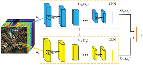
Universal distance measurement methods, such as Euclidean distance and cosine distance, are commonly used to calculate quantitative values in high-dimensional or complex data. In our approach, we train a relation network to extract features and measure the dissimilarity between them. Specifically, a pair of pixels is inputted into a CNN with the same structure, consisting of convolutional layers, pooling layers, and fully connected layers. The convolutional layer is responsible for extracting local information, and its parameters are shared across the network. The pooling layer can be implemented using various techniques, such as max pooling or average pooling. The fully connected layer connects the features from all previous layers and produces a classification result. It is important to note that the two input data points are fed into two identical neural networks, which share the same feature extraction parameters. The final feature representation is then passed to the fully connected layer, and the output is a value indicating the similarity between the two pixels.

Considering the usage of the relation network, we provide a detailed explanation of the training sample selection process. Our strategy involves combining two pixels into a single unit, and the relation network is trained to measure the similarity between these pixel pairs. It is widely accepted that samples within the same class exhibit lower distances compared to samples from different classes. This implies that if two samples belong to the same class, they should have a higher similarity. To reflect this, we assign a label of 1 to indicate high similarity for pixel pairs within the same class. Conversely, we group together pixel pairs from different classes and assign them a label of 0. The balance between positive and negative samples is crucial and needs to be carefully considered.

For instance, if an original class (class 1) contains four training pixels, combining these pixels in pairs results in six different combinations just like Figure 1. Although the increase seems modest from 4 to 6, as the number of training pixels grows, the quantity significantly increases. After grouping all pixels from each training class, we gather them together and shuffle them to obtain a large number of pixel pairs labelled as 1 (positive samples).

Figure 1. Example of pair formation.

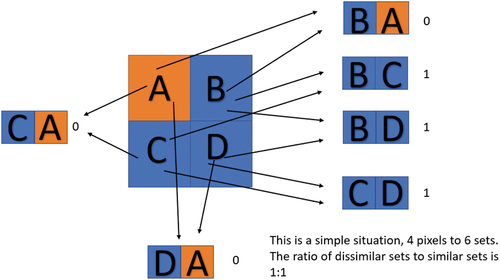
When dealing with negative pixel pairs, one pixel (pixel A) comes from a particular training class, while the other pixel comes from classes other than the one to which pixel A belongs. Combining pixel A with all pixels from other classes could lead to an excessive number of negative pixel pairs compared to positive samples, resulting in sample imbalance. This imbalance can introduce training issues, such as incorrect optimization of the classification plane. To address sample imbalance, several solutions can be employed, such as increasing the number of training samples with a small number or generating new samples based on the original training data. Another approach involves reducing the number of classes with a large amount of samples through subsampling. In our experiments, we utilized this subsampling method to mitigate sample imbalance.

To address the data imbalance problem, we group one pixel with other classes by sampling a portion of combinations from different classes based on a specific experimental probability. This approach allows us to obtain a reduced number of negative training samples and mitigate the issue of data imbalance. By sampling according to a probability distribution, we ensure monotonicity, meaning that if the training samples for a particular class are enlarged, that class will preserve more training data and have a significant influence on the final results. This probabilistic sampling strategy helps maintain a balanced representation of classes and ensures that each class has a fair contribution to the training process.

2.1.2. Train relation network

Our relation network consists of convolutional layers, pooling layers, and fully connected layers. The convolutional and pooling layers are responsible for extracting features from the input data, leading to high-level semantic representations. Its specific structure is shown in Table 1. As we go deeper into the network, the receptive field increases, allowing for the description of more complex objects. However, an increase in the number of layers and the size of convolution filters can potentially cause overfitting. To address this issue, parameter regularization and dropout techniques can be employed. Parameter regularization adds constraints to the solution space, encouraging the model to obtain simpler parameters and shrinkage values. Dropout, on the other hand, randomly deactivates neurons during forward propagation, reducing the risk of overfitting. For each pixel pair $(x_i,x_j)$, we construct a feature extraction network that maps them to a target subspace $(f(x_i),f(x_j))$, where their similarity is compared. If the two pixels belong to the same class, we aim to guide them to have similar values. Conversely, if the pixels come from different classes, we aim to guide them to have different values. The feature extraction network should have the same structure for each pixel, and their outputs are then input into the relation measure network. In our approach, we employ a fully connected layer as the relation measure method. The two feature vectors are flattened into one-dimensional vectors and concatenated along this dimension. The final output is a number ranging from 0 to 1.

Table 1. Structural parameters for feature extraction in relation network.

Layer	Input Size	Convolution	Pooling	Activation Function	Dropout
1	1$\times$200$\times$1	1$\times$9	NO	ReLu	NO
2	1$\times$192$\times$16	1$\times$3	1$\times$3	ReLu	NO
3	1$\times$63$\times$40	1$\times$3	NO	ReLu	NO
4	1$\times$61$\times$40	1$\times$3	1$\times$2	ReLu	NO
5	1$\times$29$\times$80	1$\times$3	NO	ReLu	NO
6	1$\times$27$\times$80	1$\times$3	1$\times$2	ReLu	NO
7	1$\times$12$\times$80	1$\times$12	NO	ReLu	NO
8	1$\times$1$\times$80	1$\times$1	NO	ReLu	NO
9	80	–	NO	ReLu	0.5

There are two ways to train the relation network. One approach is to make the feature extraction processes independent of each other. The two pixels of a pixel pair are fed into this feature extraction portion, ensuring weight sharing. Alternatively, a network can be designed to accept two pixels as input instead of one. This requires a two-branch feature extraction network with the same structure, ensuring equal contributions to the final result.

Figure 2 illustrates the structure of the relation network. The input data for the network consist of pairs of samples $({\mathbf{x}}_i,{\mathbf{x}}_j),(i,j)\in {\mathbb{R}}^{H\times H}$, where $H$ is the spectral dimension. The feature extraction module $G_w(\mathbf{x})$, which shares weights, extracts spectral features of the pixels in the pairs $({\mathbf{x}}_i,{\mathbf{x}}_j)$. It guides the relation network to learn the mapping relationship between their differences in the feature space and the labels of the sample pairs. The feature extraction module aims to learn spectral features of hyperspectral pixels, mapping the input data into a feature space represented by more informative advanced features.

Figure 2. Flowchart of relation network.

2.1.3. Replace portion pixels

First, we need to consider which type of data is more amenable to feature extraction and classification. When the test data exhibit a similar distribution to the training data, achieving good results on the training data usually leads to good performance on the test data as well. In the case of hyperspectral images (HSI), the energy of the image is primarily concentrated in the low-frequency and intermediate-frequency spectra, while the relevant information is often embedded in the high-frequency spectrum. Smoothing filters in the spatial domain typically calculate the average pixel value of a pixel and its neighbouring pixels. However, the size of the neighbourhood directly affects the final outcome. Increasing the filter size improves the filtering effect, but excessively large filter sizes may result in the loss of marginal information. We propose a hypothesis that simplifying and smoothing the training data can lead to easier feature extraction and classification processes, ultimately yielding better results.

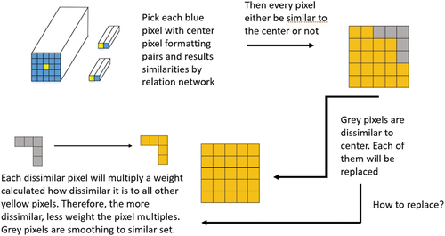
To achieve this simplification and smoothing, we employ specific strategies for each HSI cube. Instead of replacing a regular neighbour of a pixel with the same data, such as through average filtering, we focus on adjusting the overall smoothness of the cube. This approach reduces the need for extensive experimentation with different filter windows. We determine which pixels need to be modified using our trained relation network. Specifically, for each raw data cube, we combine each pixel with the centre pixel to form a pixel pair. We then feed this pair into the trained relation network, which assigns a similarity grade representing a probability. Based on whether the two pixels belong to the same class, we determine the next steps for modifying the data. Above process is shown in below Figure 3.

Figure 3. Flowchart of replace portion pixels.

For the HSI pixel patch $X_i\in R^{K\times K\times H}$, a pixel pair $(x_c,x_j)$ is constructed by combining the central pixel $x_c$ and its neighbouring pixels $x_j$. The similarity of the two elements in the combination is estimated according to the relation network, and $sim(x_c,x_j)$ is obtained. According to this information, all the pixels in the patch are divided into two sets: similar set S and dissimilar set D. The division rules are as follows:

(1) $\begin{array}{c}S=\{x_i|sim(x_c,x_j)\ge 0.5\}\\ D=\{x_i|sim(x_c,x_j)<0.5\}\end{array}$(1)

The similarity between the centre pixel, $x_c$, and the surrounding neighbourhood, $x_j$, is represented by $sim(x_c,x_j)$. Pixels $x_j$ with a similarity score greater than or equal to 0.5 are classified as belonging to the similar set, S, while those with a score below 0.5 are classified as belonging to the dissimilar set, D. The pixels in the similar set exhibit spectral properties similar to the central pixel and are more likely to belong to the same class.

To address the heterogeneity within the pixel patch, we select filling samples from the similar set, S, and use them to replace the heterogeneous regions in the pixel patch, $X_i$, resulting in a replaced pixel patch denoted as ${X_i}^{\prime }$. This filling process aims to generate a virtual pixel patch that is more similar to the central pixel while preserving the spatial continuity of the original patch. The replaced HSI pixel patch, ${X_i}^{\prime }$, enhances the similarity to the centre pixel and improves boundary classification.

For the pixels in the dissimilar set that need to be replaced, the method obtains corresponding replacement pixels from the similar set using linear weighting. The linear weighting scheme is as follows:

(2) ${x_d}^{\prime }=\sum _{s=1}^{S_L}{\alpha }_{d,s}\times x_d$(2)

$S_L$ represents the total number of similar sets, and ${x_d}^{\prime }$ denotes the replacement pixel calculated using the replacement strategy for pixel $x_d$. Pixel $x_d$ belongs to the dissimilar set D, while pixel $x_s$ belongs to the similar set S. Together, they form a pixel pair $(x_d,x_s)$. The similarity $sim(x_d,x_s)$ of this pixel pair is predicted by the trained relation network models.

The linear weight ${\alpha }_d$,s is calculated as the ratio of the similarity between the pixel to be replaced, $x_d$, and the pixel $x_s$ belonging to S, to the sum of the similarities between the pixel to be replaced, $x_d$, and all the pixels in the similar sets. Mathematically, it can be expressed as:

(3) ${\alpha }_{d,s}=\frac{sim(x_d,x_s)}{\sum _{s=1}^{S_L}sim(x_d,x_s)}$(3)

It can be observed from formula 4 that when the similarity between the pixel to be replaced, $x_d$, and the pixel $x_s$ in the similar set S is high, the weight assigned to the pixel $x_s$ in the virtual replacement pixel, ${x_d}^{\prime }$, is larger. This linear weighting approach enables the construction of virtual replacement pixels in an adaptive manner. It not only increases the similarity between the remaining pixels of the HSI pixel patch and the central pixel but also ensures the spatial consistency of local areas. Such adaptiveness and spatial consistency are beneficial to the feature extraction process of the classification network.

2.2. Classification network

Image feature extraction and classification are vital research directions in the field of computer vision. Convolutional Neural Networks (CNNs) offer an end-to-end learning model, which involves two stages in the training process. The first stage is forward propagation, where the HSI data is fed into the designed network to generate a prediction result. The second stage involves optimizing the model by combining the backpropagation algorithm with the gradient descent algorithm, based on the difference between the prediction and the true label.

In our work, we adopted a custom-designed structure (Zhang, Li, and Du 2018) based on 2D CNNs. This structure integrates local details and high-level structural information through the cross-layer aggregation of previous and deep layers. In a typical CNN model, convolutional layers with high spatial resolutions excel at capturing detailed information such as corners, edges, and colour information. On the other hand, convolutional layers with low spatial resolutions excel at capturing structural information with advanced semantics. Our design draws inspiration from Densenet and Resnet, naturally incorporating the characteristics of low, medium, and high levels of features. The richness of features increases as we deepen the network. Specifically, in our structure, the input HSI data directly propagate back to the last feature layer through a single convolutional layer, enabling the fusion of shallow information with deep semantic details. Additionally, another information stream flows into a convolutional layer and a batch normalization layer, acquiring medium-level features. It then undergoes the same operation as the low-level feature and merges with the last feature layer. Finally, in the last convolutional layer, the input is the medium-level feature, and the output combines with the other two features. To evaluate the effectiveness of the network model, we built six regions with flexible shapes in the form of diverse rectangles, followed by six blocks of CNN models as feature extractors. Each feature exhibits a similar structure to the other features. In our experiments, we selected a single global model to showcase the individual influence of the network model.

The second model is based on 3D CNN and utilizes multiple convolutional layers and pooling layers to extract deep features from HSIs. These features play a crucial role in image classification and object detection (Chen et al. 2016). By incorporating an additional dimensionality in the spectral channel, 3D CNN can effectively capture spectral-spatial information, considering both spectral and spatial characteristics simultaneously. In the structure of the 3D CNN for HSI classification, there are three layers, each consisting of a convolutional layer followed by a pooling layer. For instance, a $4\times 4\times 32$ kernel or a $3\times 3\times 32$ kernel can be applied for 3D convolution, and a $2\times 2$ kernel can be used for subsampling.

The third model we employ is a hybrid spectral convolutional neural network (HybridSN) (Roy et al. 2020) specifically designed for HSI classification. HybridSN combines spectral-spatial 3D CNN with spatial 2D CNN. The 3D CNN component enables the joint representation of spatial and spectral features by stacking spectral bands and applying 3D filters across all three dimensions. This approach overcomes the computational complexity associated with traditional 3D CNN architectures. In the HybridSN structure, each feature map in the current layer is connected to the adjacent channel of the previous layer, facilitating information flow between spectral bands. Unlike 2D CNN, which only applies convolutions over spatial dimensions, 3D CNN handles both spatial and spectral dimensions. By sliding filters along height, width, and channel dimensions, it captures spectral-spatial representations from HSI data. Although the calculation is more intricate, 3D CNN can effectively extract both spectral and spatial features. The classification framework of HybridSN consists of three 3D convolutions, one 2D convolution, and three fully connected layers. The three 3D convolutions preserve the spectral information, and after the flatten layer, a 2D convolution is applied to enhance spatial discrimination across different spectral bands.

We utilize these three widely recognized HSI classification frameworks as baseline models to validate the effectiveness and versatility of our proposed preprocessing method. Experimental results demonstrate the efficacy of our approach.

3. Experimental results and discussions

In this section, we introduce three universal HSI datasets, specify the model configuring process, and evaluate the proposed methods using classification metrics, such as overall accuracy (OA), average accuracy (AA), and kappa coefficient (kappa).

3.1. Experimental dataset

We use the IN (Indian Pines), UP (Pavia University), and KSC (Kennedy Space Center) datasets for assessing the preprocessing method.

The IN dataset, acquired by Airborne Visible/Infrared Imaging Spectrometer (AVIRIS) in 1992 from Northwest Indian, contains 16 vegetation classes and has $145\ast 145$ pixels with a spatial resolution of $20m$. Twenty bands destroyed by water absorption effect have been discarded, and the remaining 200 bands are used for evaluation, ranging from $400nm$ to $2500nm$.

The UP dataset, gathered by Reflective Optics System Imaging Spectrometer in Northern Italy in 2001, contains nine urban land-cover types and has $610\ast 340$ pixels with a spatial resolution of $1.3m$. The noisy bands have been discarded, and the remaining 103 bands are employed for evaluation, ranging from $430nm$ to $860nm$.

The KSC dataset, collected by AVIRIS in Florida in 1996, contains 13 upland and wetland classes and has $512\ast 614$ pixels with a spatial resolution of $18m$. The bands with low signal-to-noise ratio have been removed, and the remaining 176 bands are used for assessment, ranging from $400nm$ to $2500nm$.

3.2. Experimental setup

This preprocessing method is suitable for models trained and tested using image patches of size $k\times k\times n$ centred on the pixel to be classified, where k is the width and height of the patch, and n is the number of channels.

For the IN, UP, and KSC datasets, the input data sizes of the classification models are $11\times 11\times 200$, $11\times 11\times 103$, and $11\times 11\times 176$ respectively, and the raw input data was normalized between [0,1]. The IN, UP, and KSC datasets was set $10\mathrm{\%}$, $2\mathrm{\%}$, and $10\mathrm{\%}$ of the samples for training, respectively. Tables 2–4 list the specific divisions of the three datasets.

Table 2. Training and testing numbers in the Indian dataset.

Class	Training	Train	Test
1	Alfalfa	4	42
2	Corn-N	142	1286
3	Corn-M	83	747
4	Corn	23	214
5	Grass-P	48	435
6	Grass-T	73	657
7	Grass-P-M	4	24
8	Hay-W	47	431
9	Oats	4	16
10	Soybean-N	97	876
11	Soybean-M	245	2210
12	Soybean-C	59	534
13	Wheat	20	185
14	Woods	126	1139
15	Buildings-G-T	38	348
16	Stone-S-T	9	84
TOTAL		1020	9929

Table 3. Training and testing numbers in the UP dataset.

Class	Training	Train	Test
1	Asphalt	132	6499
2	Meadows	372	18277
3	Gravel	40	2059
4	Trees	60	3004
5	Sheets	26	1319
6	Bare Soil	100	4929
7	Bitumen	26	1304
8	Bricks	72	3610
9	Shadows	18	929
TOTAL		846	41930

Table 4. Training and testing numbers in the KSC dataset.

Class	Training	Train	Test
1	Scrub	76	685
2	Willow swamp	24	219
3	CP hammock	25	231
4	Slash pine	25	227
5	Oak/Broadleaf	16	145
6	Hardwood	22	207
7	Swamp	10	95
8	Graminoid marsh	43	388
9	Spartina marsh	52	458
10	Cattail marsh	40	364
11	Salt marsh	41	378
12	Mud flats	50	453
13	Water	92	935
TOTAL		515	4096

All experiments are performed on an HP desktop computer equipped with an Intel Xeon(R) Silver 4114 CPU, two GTX 2080 Ti graphics cards, and 128 GB memory. All experimental results are obtained by randomly dividing the training set and test set. The average is obtained by calculating the results of five runs. For relation network, we used the Adam optimizer with a learning rate of 0.001. The batch size was 256, and the number of training epochs was 200. The Adam optimizer was also used for training on classification tasks. The learning rate was set to 0.001, and the batch size was 64. The number of training epochs was 200.

For hyperspectral classification tasks, a limited number of training samples may lead to overfitting of the model. To solve the above problem, we adopted a simple and effective data expansion method to increase training samples without introducing additional generation labels. For each training sample, the coordinate axis was set up at the centre of the hyperspectral pixel block, and was turned horizontally and vertically to obtain the expanded training samples. After data enhancement, the number of training samples was quadrupled, effectively alleviating the problem of network overfitting.

3.3. Analysis of preprocessing effect

There is a high correlation between spectral bands in hyperspectral images, which can be measured using the Pearson coefficient and spectral angle. To assess this correlation, we consider a hyperspectral pixel block as the basic unit. We calculate the sum of Pearson distances between the central pixel and the other pixels in the block, denoted as $D_{PCC}$. Additionally, we compute the sum of spectral angular distances between the central pixel and the other pixels in the block, recorded as $D_{SAM}$. Furthermore, the variance of the spectral vectors within a hyperspectral pixel block reflects the data fluctuation. Hence, we calculate the sum of variances of the spectral vectors as an indicator of the data fluctuation within the hyperspectral pixel block. Table 5 presents the changes in Pearson coefficient, spectral angle, and mean variance values of all pixels before and after preprocessing on the three datasets. Prior to preprocessing, the input data is normalized to mitigate the influence of noise from singular data. The table reveals that the Pearson coefficient and spectral angular distance of hyperspectral image blocks have increased after the data preprocessing step, indicating an improvement in the similarity of hyperspectral image blocks. Moreover, the variance values have decreased, suggesting that the image blocks have become smoother. Consequently, the hyperspectral preprocessing method based on metric learning effectively enhances the correlation within HSI blocks and smoothens the original hyperspectral data.

Table 5. Data comparison before and after preprocessing.

	IN		UP		KSC
Index	before	after	before	after	before	after
$D_{PCC}$	119.36	120.37	102.34	106.19	113.71	115.68
$D_{SAM}$	120.18	120.71	118.81	119.41	118.26	119.17
variance	0.3084	0.1176	0.5882	0.4353	0.9321	0.3448

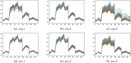
Figures 4, 5 and 6 are comparisons of three datasets before and after preprocessing. In these figures, (a), (b), and (c) are the spectrograms of three different original hyperspectral image blocks, and (d), (e), and (f) are the spectrograms of three hyperspectral image blocks after preprocessing, respectively. It can be seen that the spectral distribution of hyperspectral image blocks corresponding to figure (a) and figure (c) is complex, and the spectral distribution tends to be uniform after preprocessing. For the hyperspectral image block with uniform original distribution corresponding to figure (b), its original spectral distribution is preserved.

Figure 4. Comparison of IN dataset before and after preprocessing.

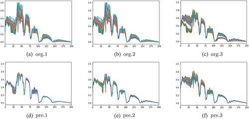
Figure 5. Comparison of UP dataset before and after preprocessing.

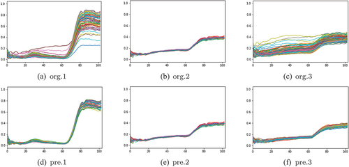
Figure 6. Comparison of KSC dataset before and after preprocessing.

To further evaluate the effectiveness of the proposed preprocessing method, a comparison is conducted based on two aspects: data smoothing and diversity preservation of hyperspectral image blocks. The IN dataset is selected for this comparative experiment.

Mean filtering is a common data smoothing method, which replaces the central pixel with the average value of neighbouring pixels. However, mean filtering treats all pixels equally and does not consider the importance of different pixels or the distribution of the original pixel block. As a result, mean filtering may not preserve the diversity and detailed information of the samples effectively.

Attention mechanisms focus on emphasizing meaningful features which can be used in the following data preprocessing comparison, and also the comparison of classification results will be addressed in the next section. Rather than mean filtering or our methods, attention mechanisms enhance or diminish the features of pixels to smooth the data rather than replacing them directly.

Figure 7 provides a visual comparison of different preprocessing methods, where the prefix ‘M’ indicates the result of mean filtering, ‘A’ indicates the result of attention mechanism, and the prefix ‘R’ indicates the result of our proposed preprocessing method. By comparing Figures 7(a), 7(b), and Figure 7(c), it is evident that the diversity of the original sample block may be lost when the spectral distribution is relatively uniform. In our method, the similarity between the central pixel and other pixels in the neighbourhood is predicted, and the decision to replace a pixel is made accordingly, thus ensuring the preservation of sample diversity. Figure 7(d) shows that the attention mechanism preserves more details than our method, particularly in the 25–50 bands.

Figure 7. Comparison of different preprocessing methods on IN dataset.

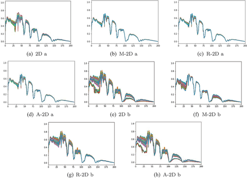
For the original hyperspectral pixel block shown in Figure 7(e) with a complex spectral distribution, Figures 7(f) & 7(g) demonstrate that both preprocessing methods can retain the main part of the pixel block and effectively smooth the data, particularly in the 0–50 bands and 100–150 bands. In Figure 7(h) attention mechanism keeps more details in 0–50 bands and 100–150 bands with less smooth result. Our preprocessing method performs local replacement based on the similarity between neighbouring pixels and the central pixel, aiming to preserve the original spectral distribution of the hyperspectral pixel blocks as much as possible while smoothing the data.

Overall, the visual comparison demonstrates that our proposed preprocessing method achieves both data smoothing and diversity preservation in hyperspectral image blocks.

3.4. Classification result and analysis

To validate the effectiveness of the proposed preprocessing method, a comparative analysis of the replacement is conducted on three classification models: 2D CNN (Zhang, Li, and Du 2018), 3D CNN (Chen et al. 2016), and HySN (Roy et al. 2020). In the classification results, the prefix ‘R’ indicates that the input data is preprocessed. For reaching the best performance of our method, a data augmentation method is employed to increase the training dataset without the need for introducing additional generated labels with R-HySN model which is theoretically better than R-2D CNN and R-3D CNN label as ‘AR-HySN’. For each training sample, we establish a coordinate axis at the centre of the hyperspectral pixel block and perform horizontal and vertical flips separately, resulting in augmented training samples. After data augmentation, the number of training samples becomes four times the original, effectively alleviating the problem of network overfitting.

Tables 6–8 present the overall accuracy (OA), average accuracy (AA), and Kappa coefficient for HSI classification, as well as the classification accuracies for all categories. The results obtained using the replacement preprocessing method demonstrate higher classification performance compared to the baseline method. Furthermore, the classification maps are visually represented in Figures 8–10.

Figure 8. Plot of classification results for the IN dataset.

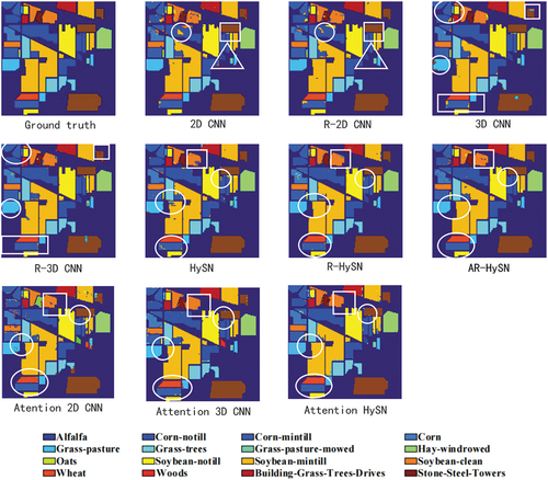
Figure 9. Plot of classification results for the UP dataset.

Figure 10. Plot of classification results for the KSC dataset.

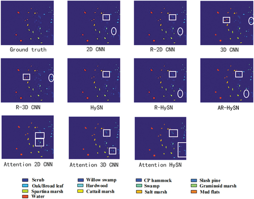
Table 6. Classification results of different methods for the IN dataset.

Class	2D CNN	R-2D CNN	A-2D CNN	3D CNN	R-3D CNN	A-3D CNN	HySN	R-HySN	AR-HySN	A-HySN
1	82.5$\pm$8.9	93.4$\pm$6.4	97.5$\pm$6.0	92.7$\pm$9.6	93.6$\pm$6.1	100$\pm$0.0	94.4$\pm$4.5	95.2$\pm$3.5	95.3$\pm$2.3	94.7$\pm$4.0
2	92.1$\pm$2.3	92.9$\pm$2.3	95.4$\pm$0.8	95.4$\pm$2.6	96.8$\pm$2.0	97.7$\pm$4.3	93.5$\pm$3.4	95.8$\pm$1.8	98.6$\pm$1.6	97.4$\pm$5.1
3	93.6$\pm$1.2	94.0$\pm$4.8	87.3$\pm$9.9	96.2$\pm$1.8	97.2$\pm$2.0	92.6$\pm$2.7	94.3$\pm$0.9	93.9$\pm$2.3	97.7$\pm$1.3	99.0$\pm$2.7
4	75.2$\pm$5.1	78.0$\pm$8.3	90.6$\pm$1.0	92.5$\pm$4.5	96.7$\pm$3.0	87.3$\pm$2.3	82.4$\pm$4.0	91.7$\pm$2.4	91.5$\pm$1.8	95.3$\pm$5.2
5	93.3$\pm$4.5	94.7$\pm$3.3	85.2$\pm$5.3	87.9$\pm$3.3	92.2$\pm$3.8	92.8$\pm$5.7	95.7$\pm$2.0	96.5$\pm$3.9	96.6$\pm$2.6	93.6$\pm$5.7
6	98.9$\pm$2.0	99.2$\pm$1.7	93.2$\pm$9.2	95.2$\pm$2.2	99.3$\pm$0.6	94.9$\pm$6.9	99.4$\pm$0.1	99.5$\pm$0.5	98.8$\pm$1.1	93.3$\pm$6.1
7	80.0$\pm$6.8	85.5$\pm$9.8	100$\pm$0.0	86.7$\pm$8.2	92.0$\pm$9.8	92.0$\pm$0.0	81.9$\pm$5.1	87.7$\pm$6.5	87.5$\pm$4.1	92.3$\pm$1.8
8	99.6$\pm$1.4	99.8$\pm$0.2	100$\pm$0.0	99.8$\pm$0.2	99.9$\pm$0.2	100$\pm$0.0	100$\pm$0.0	100$\pm$0.0	100$\pm$0.0	99.0$\pm$3.4
9	85.6$\pm$8.7	87.5$\pm$9.1	76.4$\pm$7.0	77.2$\pm$8.0	76.7$\pm$9.6	74.7$\pm$0.5	87.0$\pm$9.3	88.0$\pm$9.6	87.3$\pm$7.6	85.0$\pm$0.9
10	93.7$\pm$2.3	97.8$\pm$3.8	94.7$\pm$3.6	91.2$\pm$1.7	95.6$\pm$2.0	98.1$\pm$6.9	95.4$\pm$1.2	96.2$\pm$1.0	95.9$\pm$1.4	98.9$\pm$2.1
11	97.1$\pm$2.1	97.4$\pm$2.0	97.1$\pm$0.2	97.6$\pm$0.9	96.3$\pm$1.5	99.0$\pm$9.4	98.2$\pm$0.9	99.0$\pm$0.6	98.7$\pm$0.9	97.8$\pm$7.0
12	87.4$\pm$6.2	95.1$\pm$8.0	95.1$\pm$2.1	93.1$\pm$3.1	93.3$\pm$3.1	89.1$\pm$1.8	91.8$\pm$1.2	93.6$\pm$0.8	94.2$\pm$2.7	96.5$\pm$2.3
13	94.2$\pm$6.6	98.4$\pm$4.3	91.3$\pm$0.4	96.6$\pm$3.6	95.8$\pm$3.7	99.4$\pm$5.6	99.2$\pm$0.6	98.9$\pm$0.3	99.2$\pm$0.1	100$\pm$0.0
14	98.2$\pm$1.2	99.2$\pm$1.5	97.7$\pm$1.5	98.8$\pm$0.9	99.5$\pm$0.4	99.5$\pm$6.0	99.3$\pm$0.7	99.2$\pm$0.5	99.8$\pm$0.2	99.1$\pm$8.7
15	94.1$\pm$1.7	93.7$\pm$5.6	93.0$\pm$8.3	90.0$\pm$7.0	98.6$\pm$1.1	98.5$\pm$5.9	95.0$\pm$2.3	95.6$\pm$1.4	95.5$\pm$0.9	98.7$\pm$7.2
16	84.6$\pm$1.7	84.5$\pm$8.1	91.5$\pm$6.6	86.5$\pm$5.3	87.4$\pm$10.0	96.3$\pm$8.5	97.6$\pm$1.9	93.7$\pm$4.0	94.0$\pm$1.6	87.5$\pm$0.2
OA	94.5$\pm$0.8	96.0$\pm$0.4	94.6$\pm$2.8	95.3$\pm$0.5	96.7$\pm$0.4	96.8$\pm$4.2	96.2$\pm$0.2	97.1$\pm$0.2	97.5$\pm$0.1	97.4$\pm$4.3
AA	90.6$\pm$1.4	93.2$\pm$1.2	92.9$\pm$1.4	92.0$\pm$1.2	94.5$\pm$0.8	93.9$\pm$1.0	94.1$\pm$1.6	95.3$\pm$0.5	95.6$\pm$0.2	95.5$\pm$0.0
Kappa	93.7$\pm$1.7	95.3$\pm$1.1	93.8$\pm$7.0	94.6$\pm$0.4	96.3$\pm$0.4	96.3$\pm$9.5	95.9$\pm$0.9	96.5$\pm$0.4	97.1$\pm$0.3	97.0$\pm$8.7

Table 7. Classification results of different methods for the UP dataset.

Class	2D CNN	R-2D CNN	A-2D CNN	3D CNN	R-3D CNN	A-3D CNN	HySN	R-HySN	AR-HySN	A-HySN
1	94.2$\pm$1.8	96.3$\pm$1.5	93.4$\pm$0.4	96.5$\pm$0.8	97.9$\pm$0.4	98.3$\pm$8.2	97.7$\pm$1.5	98.0$\pm$0.3	98.3$\pm$0.4	96.4$\pm$7.1
2	98.5$\pm$0.3	97.8$\pm$0.3	99.0$\pm$9.8	98.4$\pm$0.4	98.1$\pm$0.8	95.1$\pm$3.4	97.6$\pm$1.7	99.0$\pm$0.3	99.2$\pm$0.7	99.0$\pm$2.0
3	75.4$\pm$2.9	84.9$\pm$6.1	90.0$\pm$7.4	73.1$\pm$9.4	90.2$\pm$3.6	90.7$\pm$2.7	89.2$\pm$1.6	94.3$\pm$4.5	92.4$\pm$1.1	92.5$\pm$9.4
4	92.1$\pm$0.6	97.8$\pm$0.5	96.3$\pm$1.2	97.1$\pm$1.4	95.9$\pm$2.0	97.2$\pm$7.0	94.7$\pm$1.4	95.4$\pm$2.7	95.7$\pm$1.3	99.0$\pm$5.1
5	99.8$\pm$0.2	99.7$\pm$0.2	99.7$\pm$6.8	99.8$\pm$0.2	99.9$\pm$0.1	99.8$\pm$6.4	99.9$\pm$0.1	100$\pm$0.0	100$\pm$0.0	100$\pm$0.0
6	90.0$\pm$1.1	92.4$\pm$2.5	90.4$\pm$9.8	93.9$\pm$2.2	93.9$\pm$3.0	92.0$\pm$0.7	95.4$\pm$1.1	97.6$\pm$3.0	97.4$\pm$0.8	98.8$\pm$0.2
7	84.5$\pm$4.6	91.6$\pm$6.6	84.4$\pm$1.1	85.1$\pm$4.8	96.1$\pm$2.8	97.5$\pm$3.7	97.7$\pm$1.6	92.7$\pm$2.3	96.2$\pm$1.0	95.4$\pm$5.6
8	87.9$\pm$2.7	96.1$\pm$2.3	83.9$\pm$8.5	90.2$\pm$1.3	91.1$\pm$3.8	96.5$\pm$9.2	89.3$\pm$1.1	90.7$\pm$1.6	94.0$\pm$1.5	95.0$\pm$2.9
9	97.6$\pm$2.2	96.2$\pm$2.2	94.8$\pm$5.2	94.4$\pm$0.1	97.5$\pm$2.7	96.5$\pm$8.4	96.4$\pm$1.4	93.8$\pm$0.8	97.6$\pm$0.9	80.6$\pm$0.4
OA	94.4$\pm$0.7	96.0$\pm$0.5	94.7$\pm$3.2	95.0$\pm$0.5	96.4$\pm$0.6	95.5$\pm$8.7	96.1$\pm$0.5	97.2$\pm$0.2	97.7$\pm$0.2	97.3$\pm$9.9
AA	91.6$\pm$1.1	94.7$\pm$0.8	92.4$\pm$8.9	92.1$\pm$0.8	95.6$\pm$0.7	90.0$\pm$0.6	95.3$\pm$0.5	95.7$\pm$0.4	96.7$\pm$0.3	95.3$\pm$1.2
Kappa	92.8$\pm$0.8	95.7$\pm$0.6	92.9$\pm$9.4	93.5$\pm$0.6	95.3$\pm$0.7	94.1$\pm$7.4	94.8$\pm$0.7	96.3$\pm$0.3	97.0$\pm$0.2	96.5$\pm$4.8

Table 8. Classification results of different methods for the KSC dataset.

Class	2D CNN	R-2D CNN	A-2D CNN	3D CNN	R-3D CNN	A-3D CNN	HySN	R-HySN	AR-HySN	A-HySN
1	99.8$\pm$0.2	99.5$\pm$0.8	99.0$\pm$7.2	99.8$\pm$0.1	99.9$\pm$0.1	97.6$\pm$5.2	99.9$\pm$0.1	99.9$\pm$0.1	99.8$\pm$0.2	98.9$\pm$6.7
2	92.8$\pm$5.1	97.4$\pm$1.1	91.4$\pm$6.2	97.0$\pm$1.1	97.1$\pm$0.4	96.3$\pm$6.5	97.0$\pm$1.0	97.7$\pm$0.7	97.7$\pm$0.3	93.5$\pm$0.1
3	93.7$\pm$7.2	94.4$\pm$6.1	99.8$\pm$0.2	97.6$\pm$7.1	97.4$\pm$1.5	96.3$\pm$6.2	95.0$\pm$6.2	95.4$\pm$0.9	96.1$\pm$5.3	94.4$\pm$0.5
4	75.9$\pm$9.7	77.1$\pm$5.3	86.3$\pm$9.9	75.9$\pm$8.2	87.8$\pm$8.1	83.5$\pm$7.9	82.5$\pm$6.1	84.1$\pm$5.5	88.5$\pm$8.4	95.0$\pm$0.9
5	75.2$\pm$8.1	82.3$\pm$4.4	88.7$\pm$9.7	81.5$\pm$5.6	80.7$\pm$6.2	93.5$\pm$1.5	81.9$\pm$3.8	83.7$\pm$4.6	85.1$\pm$2.9	91.0$\pm$3.2
6	89.7$\pm$9.5	92.5$\pm$3.6	93.0$\pm$4.5	88.6$\pm$4.0	90.5$\pm$8.6	87.6$\pm$0.8	92.0$\pm$3.4	92.7$\pm$6.3	94.8$\pm$2.7	99.1$\pm$0.8
7	89.1$\pm$5.3	93.7$\pm$6.9	84.8$\pm$8.6	90.9$\pm$5.6	89.7$\pm$3.4	100$\pm$0.0	94.7$\pm$5.6	97.9$\pm$3.6	97.2$\pm$4.9	89.2$\pm$9.7
8	94.4$\pm$2.8	97.3$\pm$1.6	96.9$\pm$4.2	97.1$\pm$1.4	97.4$\pm$2.3	94.9$\pm$5.5	98.1$\pm$2.5	98.3$\pm$2.1	97.3$\pm$1.8	93.8$\pm$9.2
9	99.5$\pm$0.5	99.0$\pm$0.4	97.5$\pm$9.7	98.9$\pm$0.6	99.6$\pm$0.4	98.4$\pm$4.7	98.9$\pm$0.9	99.6$\pm$1.2	99.6$\pm$0.3	100$\pm$0.0
10	98.9$\pm$1.9	99.5$\pm$1.0	90.0$\pm$7.9	99.3$\pm$1.5	99.6$\pm$0.8	97.5$\pm$5.2	99.5$\pm$1.1	98.8$\pm$2.1	100$\pm$0.0	97.5$\pm$5.7
11	99.8$\pm$0.2	99.6$\pm$0.6	98.9$\pm$8.4	99.7$\pm$0.3	99.6$\pm$0.3	99.5$\pm$3.1	99.9$\pm$0.1	99.8$\pm$0.2	99.6$\pm$0.3	99.5$\pm$3.1
12	98.7$\pm$1.8	98.5$\pm$1.2	96.7$\pm$1.3	98.8$\pm$1.5	98.4$\pm$1.4	99.6$\pm$0.4	98.8$\pm$1.8	99.0$\pm$0.9	99.6$\pm$0.3	98.8$\pm$0.6
13	99.6$\pm$0.7	99.8$\pm$0.3	99.6$\pm$8.2	99.8$\pm$0.5	99.9$\pm$0.3	100$\pm$0.0	99.8$\pm$0.3	99.8$\pm$0.3	100$\pm$0.0	99.7$\pm$8.1
OA	95.9$\pm$0.6	96.8$\pm$0.3	95.9$\pm$7.0	96.6$\pm$0.5	97.4$\pm$0.2	96.8$\pm$5.3	97.3$\pm$0.8	97.6$\pm$0.2	98.0$\pm$0.2	97.5$\pm$8.2
AA	92.9$\pm$1.0	94.7$\pm$0.5	94.4$\pm$3.9	94.0$\pm$0.5	95.2$\pm$0.3	95.3$\pm$4.4	95.2$\pm$1.1	95.9$\pm$0.4	96.6$\pm$0.2	96.2$\pm$3.5
Kappa	95.5$\pm$0.5	96.7$\pm$0.3	95.5$\pm$1.3	96.2$\pm$0.5	96.9$\pm$0.1	96.4$\pm$9.6	96.7$\pm$0.9	97.4$\pm$0.2	97.8$\pm$0.3	97.3$\pm$0.7

Table 6 shows the classification results of the IN dataset. For the IN dataset, the overall accuracy (OA) shows improvement when our preprocessing method is applied in most experiments, particularly for models with a lower baseline, such as 2D CNN and 3D CNN. Upon analysing the classification results of 2D CNN and 3D CNN, it becomes evident that 3D CNN outperforms 2D CNN in terms of classification performance. This can be attributed to the fact that 3D CNN utilizes 3D convolution and excels at extracting joint features from both spatial and spectral dimensions. By utilizing the preprocessed hyperspectral input data, both 2D CNN and 3D CNN exhibit noticeable enhancements in OA. The primary reason behind this improvement is that the preprocessed hyperspectral pixel blocks exhibit smoother characteristics, reducing the adverse effects caused by noise during the feature extraction process. As a result, the boundary classification is enhanced, leading to improved classification accuracy. Furthermore, the classification accuracy of HySN is relatively high, and even after applying our preprocessing method, the OA still shows a $0.9\mathrm{\%}$ improvement. This observation verifies the effectiveness of the preprocessing method in enhancing hyperspectral classification results. For the comparison between our method and attention mechanism, our method has better accuracy.

Figure 8 displays the classification results of each method on the IN dataset, with Figure 8 2D CNN and R-2D CNN showcasing the results of 2D CNN before and after preprocessing, respectively. It is evident that the classification errors of Corn-notill and grass pasture are significantly reduced as circled in Figure 8 2D CNN and 8 3D CNN, leading to an improved classification effect. This improvement can be attributed to the preprocessing step, where heterogeneous areas within the pixel block surrounding the boundary pixels are replaced with homogeneous areas. Not only boundary pixels but also inner part of pixels are replaced with homogeneous pixels increasing the consistency of classification aligned with the ground truth. This improvement enhances the consistency of image blocks, thereby correctly classifying certain points that were previously misclassified due to poor consistency.

In Figure 8 3D CNN and R-3D CNN, the improvement of preprocessing with 3D CNN is demonstrating. The boundary classification effect is also enhanced to varying degrees, and the presence of classification noise is noticeably reduced. The Stone-Steel-Towers, Grass-pasture, and corn-notill are better classified with the enhancement of preprocessing as highlighted in Figure 8. This can be attributed to the smoother nature of the preprocessed hyperspectral pixel blocks, which enables more comprehensive extraction of classification features. Consequently, the impact of classification noise is mitigated. Therefore, for the IN dataset, the proposed preprocessing method proves effective in improving boundary classification accuracy and reducing classification noise through the replacement of original hyperspectral pixel blocks.

In Figure 8 HySN, R-HySN, and AR-HySN, the improvement of preprocessing and enhancement of data with HySN CNN is demonstrating. The Soybean-mintill, Soybean-clean, and corn-notill are better classified with the enhancement of preprocessing as highlighted in Figure 8. The input data enhancement with data preprocessing performs the best in reducing classification noise.

Compared to the attention mechanism, our method deals better in various ways. For 2D CNN, we have better classification accuracy in grass-pasture as circled in Figure 8. Corn-notill with blue circled on 2D CNN plot and Stone-Steel-Towers part we all outperform attention network substantially. In terms of 3D CNN, our method excels at grass-pasture and left up corner corn-mintill part. For the best HySN model, our classification is better in left down circled area including wheat and corn-mintill and the yellow soybean-notill part.

For the UP dataset, Table 7 demonstrates that the classification metrics for the same base model have improved to varying degrees after applying the preprocessing method. The three base models utilize preprocessed input data, resulting in an increase in OA by $1.6\mathrm{\%}$, $1.4\mathrm{\%}$, and $1.1\mathrm{\%}$, respectively. The primary reason behind this improvement is that the preprocessing step facilitates a smoother spectral distribution of hyperspectral pixel blocks. As a result, effective and stable classification features can be extracted, ultimately enhancing the overall classification accuracy. Furthermore, it is worth noting that this method effectively reduces the standard deviation in the classification results while simultaneously improving classification accuracy. This indicates the robustness and stability of the proposed preprocessing method. Attention CNN performs slightly better than our method in 2D CNN. However, in 3D CNN and AR-HySN model, our method outperforms it even when its accuracy is very impressive.

Figure 9 presents the classification results of each method on the UP dataset. Specifically, Figure 9 2D CNN, R-2D CNN depicts the visual classification images of 2D CNN before and after preprocessing, respectively, as highlighted in Figure 9. In Figure 9 2D CNN, noticeable concentrated noise is observed in the boundary and inner part of Bare Soil and Gravel area. In Figure 9 R-2D CNN, the number of noise points in this area is significantly reduced. The primary reason for this improvement is that the preprocessing of hyperspectral pixel blocks mitigates the negative influence of heterogeneous areas within the block on the classification results. Consequently, this preprocessing step facilitates the extraction of stable classification features, thereby reducing classification noise. When comparing the classification results of 2D CNN and 3D CNN under the same input data, it is evident that 2D CNN combines features at different levels but does not fully utilize the joint features of spatial and spectral information. As a result, its classification performance is inferior to that of 3D CNN. In Figure 9 R-HySN, and AR-HySN, also in boundary and inner part of the area of Gravel and Bare Soil are classified better through data preprocessing than no preprocessing HySN and input data enhancement as highlighted. Therefore, for the UP dataset, this preprocessing method proves effective in reducing classification noise by replacing the original hyperspectral pixel block. For comparison with attention mechanism, in terms of 2D CNN model, the classifications of Gravel Bare Soil are very impressive. Our method has little edges in Self-Blocking Bricks and Trees area. For 3D CNN, our model provides equally good accuracy in Gravel area and with better accuracy in Meadows area. For AR-HySN model, we have edges in Asphalt and Gravel area, and attention mechanism provides a very accurate classification result as well.

Table 8 reveals that the utilization of preprocessed input data leads to varying degrees of improvement in the classification accuracy of different basic models on the KSC dataset. The overall accuracies (OAs) of the three basic models show increments of $0.9\mathrm{\%}$, $0.8\mathrm{\%}$, and $0.3\mathrm{\%}$, respectively. This improvement can be attributed to the smoothing effect on the spectral distribution of hyperspectral pixel blocks achieved through preprocessing. By reducing the complexity of the feature extraction process, the preprocessing method enhances the classification accuracy. For the comparison with attention mechanism, our method outperforms it with more accurate classification result in all models. Figure 10 illustrates the classification results of each method applied to the KSC dataset. This dataset exhibits a relatively scattered sample distribution, resulting in favourable boundary classification and overall classification effects. Figure 10 2D CNN and R-2D CNN present the classification outcomes of 2D CNN before and after preprocessing as shown in Figure 10, respectively. It is noticeable that the classification errors in the SlashPine areas near the upper right and lower right corners are significantly reduced, leading to an improved boundary classification effect. This improvement can be attributed to the increased regional consistency of hyperspectral image blocks during the preprocessing phase, which facilitates the extraction of salient features from boundary pixels and enhances the boundary classification effect. Similar improvements in the boundary classification effect can be observed in Figure 10 3D CNN and R-3D CNN highlighted above showing that Mud flats and Hardwood area are sharply classified with data preprocessing. Figure 10 HySN, R-HySN, and AR-HySN demonstrated a more prominent classification through data preprocessing and input data enhancement. These comparisons are highlighted in Figure 10. The comparison of the classification results of the same model before and after preprocessing reveals that the post-preprocessing outcomes exhibit more precise and accurate edge divisions. Consequently, for the KSC dataset, the proposed preprocessing method, involving the replacement of the original hyperspectral pixel block, effectively enhances the boundary classification effect. For compassion with attention, our method provides a more accurate classification in Hardwood area. For 3D CNN model, in the plot of attention 3D CNN, the squared Hardwood area also demonstrates that our method has little edges against attention. For HySN, apparent in two squares area (Attention HySN plot), attention mechanism gives a worse classification result than our method.

4. Conclusion

To mitigate the challenges associated with the complexity of original hyperspectral images (HSI) during training, this paper proposes a preprocessing method for HSI classification based on metric learning. The method consists of several steps. First, a relation network is designed to measure the similarity between pixels. This network enables the calculation of similarity scores among pixels within the HSI. Subsequently, based on predefined replacement rules, heterogeneous regions within non-uniform pixel patches are replaced with more homogeneous areas. This replacement process aims to enhance regional consistency within the pixel patches. Finally, the processed HSI pixel patches are fed into a classification network to extract features and accomplish the classification task. Through the pre-processing method proposed in this paper, interference information in the image patch is reduced, allowing the network to focus more on the central pixel features, which are indicative of category information during the classification task. The proposed method demonstrates improved regional consistency and enhanced boundary discrimination ability on three well-known HSI datasets. It effectively improves the boundary classification performance by reducing noise and enhancing the overall quality of the pixel patches. Compared to well-known state-of-the-art attention mechanism, our method nearly outperforms it in all scenarios, demonstrating the strong ability of our method. Importantly, the method exhibits generality and can be potentially applied to other classification models.

Additional information

Funding

This work was supported in part by the National Science Foundation of China under Grant 61877066, in part by the Aero-Science Fund under Grant 20175181013 and in part by the Science and technology plan project of Xi’an under Grant 21RGZN0010. (Corrsponding author: Xiaohua Zhang)

References

- Borana, S. L., S. R. Yadav, and S. Parihar, 2019. “Hyperspectral Data Analysis for Arid Vegetation Species: Smart Sustainable Growth.” 2019 International Conference on Computing, Communication, and Intelligent Systems (ICCCIS) 495500. Greater Noida, India: IEEE.
- Camps-Valls, G., L. Gomez-Chova, J. Munoz-Mari, J. Vila-Frances, and J. Calpe-Maravilla. 2006. “Composite Kernels for Hyperspectral Image Classification.” IEEE Geoscience and Remote Sensing Letters 3 (1): 93–97. https://doi.org/10.1109/LGRS.2005.857031.
- Chen, Y., H. Jiang, C. Li, X. Jia, and P. Ghamisi. 2016. “Deep Feature Extraction and Classification of Hyperspectral Images Based on Convolutional Neural Networks.” IEEE Transactions on Geoscience and Remote Sensing 54 (10): 6232–6251. https://elib.dlr.de/106352/2/CNN.pdf.
- Chen, Y., Z. Lin, X. Zhao, G. Wang, and Y. Gu. 2014. “Deep Learning-Based Classification of Hyperspectral Data.” IEEE Journal of Selected Topics in Applied Earth Observations and Remote Sensing 7 (6): 2094–2107. https://doi.org/10.1109/JSTARS.2014.2329330.
- Chen, Y., N. M. Nasrabadi, and T. D. Tran. 2013. “Hyperspectral Image Classification via Kernel Sparse Representation.” IEEE Transactions on Geoscience and Remote Sensing 51 (1): 217–231. https://doi.org/10.1109/TGRS.2012.2201730.
- Chen, Y., X. Zhao, and X. Jia. 2015. “Spectral–Spatial Classification of Hyperspectral Data Based on Deep Belief Network.” IEEE Journal of Selected Topics in Applied Earth Observations and Remote Sensing 8 (6): 2381–2392. https://ieeexplore.ieee.org/document/7018910/.
- Demir, B., and S. Erturk. 2009. “Clustering-Based Extraction of Border Training Patterns for Accurate Svm Classification of Hyperspectral Images.” IEEE Geoscience and Remote Sensing Letters 6 (4): 840–844. https://doi.org/10.1109/LGRS.2009.2026656.
- Duan, P., J. Lai, J. Kang, X. Kang, P. Ghamisi, and S. Li. 2020. “Texture-Aware Total Variation-Based Removal of Sun Glint in Hyperspectral Images.” The ISPRS Journal of Photogrammetry and Remote Sensing 166:359–372. https://doi.org/10.1016/j.isprsjprs.2020.06.009.
- Fauvel, M., Y. Tarabalka, J. A. Benediktsson, J. Chanussot, and J. C. Tilton. 2013. “Advances in Spectral-Spatial Classification of Hyperspectral Images.” Proceedings of the IEEE 101 (3): 652–675. https://doi.org/10.1109/JPROC.2012.2197589.
- Ge, Z., G. Cao, Y. Zhang, X. Li, H. Shi, and P. Fu. 2022. “Adaptive Hash Attention and Lower Triangular Network for Hyperspectral Image Classification.” IEEE Transactions on Geoscience Remote Sensing 60:1–19. https://doi.org/10.1109/TGRS.2021.3075546.
- Gomez-Chova, L., D. Tuia, G. Moser, and G. Camps-Valls. 2015. “Multimodal Classification of Remote Sensing Images: A Review and Future Directions.” Proceedings of the IEEE 103 (9): 1560–1584. https://doi.org/10.1109/JPROC.2015.2449668.
- Hotelling, H. 1933. “Analysis of a Complex of Statistical Variables into Principal Components.” Journal of Educational Psychology 24 (7): 498–520. https://doi.org/10.1037/h0070888.
- Hu, W., Y. Huang, L. Wei, F. Zhang, and H. Li. 2015. “Deep Convolutional Neural Networks for Hyperspectral Image Classification.” Journal of Sensors 2015:e258619. https://doi.org/10.1155/2015/258619.
- Kumar, B., O. Dikshit, A. Gupta, and M. K. Singh. 2020. “Feature Extraction for Hyperspectral Image Classification: A Review.” International Journal of Remote Sensing 41 (16): 6248–6287. https://doi.org/10.1080/01431161.2020.1736732.
- Kuo, B. C., C. S. Huang, C. C. Hung, Y. L. Liu, and I. L. Chen. 2010. Spatial Information Based Support Vector Machine for Hyperspectral Image Classification.
- Landgrebe, D. 2002. “Hyperspectral Image Data Analysis.” IEEE Signal Processing Magazine 19 (1): 17–28. https://doi.org/10.1109/79.974718.
- Melgani, F., and L. Bruzzone. 2002. Support Vector Machines for Classification of Hyperspectral Remote-Sensing Images.
- Roy, S. K., G. Krishna, S. R. Dubey, and B. B. Chaudhuri. 2020. “HybridSN: Exploring 3-D–2-D CNN Feature Hierarchy for Hyperspectral Image Classification.” IEEE Geoscience and Remote Sensing Letters 17 (2): 277–281. https://doi.org/10.1109/LGRS.2019.2918719.
- Sharma, S., and K. M. Buddhiraju. 2018. “Spatial–Spectral Ant Colony Optimization for Hyperspectral Image Classification.” International Journal of Remote Sensing 39 (9): 2702–2717. https://doi.org/10.1080/01431161.2018.1430403.
- Wang, D., B. Du, and L. Zhang. 2022. “Fully Contextual Network for Hyperspectral Scene Parsing.” IEEE Transactions on Geoscience and Remote Sensing 60:1–16. https://doi.org/10.1109/tgrs.2021.3050491.
- Wang, X., L. Ma, and F. Liu. 2013. Laplacian Support Vector Machine for Hyperspectral Image Classification by Using Manifold Learning Algorithms. IEEE International Geoscience and Remote Sensing Symposium, 1027–1030. Melbourne, VIC, Australia, 2013. https://doi.org/10.1109/IGARSS.2013.6721338
- Xue, Z., S. Yang, and L. Zhang. 2021. “Weighted Sparse Graph Regularization for Spectral–Spatial Classification of Hyperspectral Images.” IEEE Geoscience and Remote Sensing Letters 18 (9): 1630–1634. https://doi.org/10.1109/LGRS.2020.3005168.
- Yokoya, N., Z. Han, J. Yao, L. Gao, B. Zhang, A. Plaza, and J. Chanussot. 2021. “Spectralformer: Rethinking Hyperspectral Image Classification with Transformers.” IEEE Transactions on Geoscience and Remote Sensing. 60:1–15. https://doi.org/10.1109/tgrs.2021.3130716.
- Yu, C., M. Zhao, M. Song, Y. Wang, F. Li, R. Han, and C. I. Chang. 2019. “Hyperspectral Image Classification Method Based on CNN Architecture Embedding with Hashing Semantic Feature.” IEEE Journal of Selected Topics in Applied Earth Observations and Remote Sensing 12 (6): 1866–1881. https://doi.org/10.1109/JSTARS.2019.2911987.
- Zhang, S., and S. Li. 2016. Spectral-Spatial Classification of Hyperspectral Images via Multiscale Superpixels Based Sparse Representation.
- Zhang, M., W. Li, and Q. Du. 2018. “Diverse Region-Based CNN for Hyperspectral Image Classification.” IEEE Transactions on Image Processing 27 (6): 2623–2634. https://doi.org/10.1109/TIP.2018.2809606.
- Zhang, L., L. Zhang, and B. Du. 2016. “Deep Learning for Remote Sensing Data: A Technical Tutorial on the State of the Art.” IEEE Geoscience and Remote Sensing Magazine 4 (2): 22–40. https://doi.org/10.1109/MGRS.2016.2540798.