Uniform upscaling techniques for eddy covariance FLUXes (UFLUX)

ABSTRACT

Data-driven techniques that scale up eddy covariance (EC) fluxes from tower footprints with satellite observations and machine learning algorithms significantly advance our understanding of global carbon, water, and energy cycles. However, few upscaling approaches take a consistent approach to upscaling both carbon and energy fluxes. A lack of uniformity in the upscaling approach could lead to inconsistencies in global interannual variability of fluxes and between types of carbon and energy fluxes. Hence, this study aims to identify obstacles in flux upscaling and propose a uniform upscaling framework UFLUX for gross primary productivity (GPP), ecosystem respiration (Reco), net ecosystem exchange (NEE), sensible heat (H), and latent energy (LE). The key findings are as follows: 1) The upscaling performance exhibits a limited improvement from the use of more advanced machine learning approaches (e.g. <0.3 in R² improvements while using deep neural networks). 2) The spatial density of EC towers is the primary factor determining the effectiveness of upscaling, explaining >50% of the upscaling uncertainty. 3) The UFLUX framework considered the interconnection between fluxes and achieved a competitive validation precision (daily R² = 0.7 on average of five flux types) when compared with products that upscaled a subset of the fluxes. UFLUX effectively preserved the ecosystem light-use efficiency (0.83 of linear regression slope and the same after), Bowen ratio (0.8), and particularly, the water-use efficiency (0.81), when compared to the only other product (i.e. FLUXCOM) to upscale both carbon and water.

KEYWORDS:

• Remote sensing
• eddy covariance
• machine learning
• carbon cycles

1. Introduction

The EC networks have contributed greatly to our understanding of global carbon, water, and energy cycles (Baldocchi 2020). EC provides direct and continuous measurements of ecosystem-atmosphere mass and energy fluxes and has been widely used for studying ecosystem responses to environmental forcings (Reichstein et al. 2014), for validating Earth-observing satellite-derived products (Baldocchi et al. 2001), and the development, calibration and evaluation of land surface models (LSMs) (Fisher and Koven 2020). Satellite and LSMs products are not devoid of errors (Slevin 2016; Wang et al. 2017) and these errors have presented difficulties in generating reliable climate projections (H. Wang et al. 2017). Hence, accurate global flux estimates upscaled from EC networks are necessary to independently validate and bolster our climate mitigation endeavours (Jung et al. 2017).

The EC upscaling studies have achieved important breakthroughs in global ecosystem carbon uptake estimation (Beer et al. 2010), but several challenges remain. The motivation to develop a consistent and uniform EC flux upscaling was underlined by the significant disparities observed in global estimates of carbon fluxes, particularly in their GPP interannual variability (Dong et al. 2022). The divergent trends displayed by these GPP products pose significant challenges in understanding global carbon budgets and addressing the climate change crisis (Dong et al. 2022). Given the similarity of driving data, it is likely that the differences are due to the technical implementation of upscaling algorithms.

The precise influence of these technical factors on the substantial variance observed in the interannual variability of global fluxes (Dong et al. 2022) remains undetermined. Employing basic averages of outcomes obtained through the utilization of diverse driver datasets, algorithms, and so on may result in a flux time series at the global scale that exhibits little sensitivity to interannual fluctuations. Moreover, it is important to recognize that the carbon cycling processes are intricately intertwined with those of water and energy (e.g. light-use and water-use efficiencies), given that photosynthesis is significantly influenced by atmospheric and soil moisture deficits (Fu et al. 2022). Upscaling approaches that focus on single fluxes are unlikely to preserve known trends between fluxes.

Most EC upscaling studies focused on GPP (Joiner and Yoshida 2020; Ueyama et al. 2013). Whilst EC typically measures H, LE and NEE, it can be further partitioned into GPP and Reco (Aubinet, Vesala, and Papale 2012). Using a uniform upscaling routine – e.g. the same machine-learning algorithms, satellite vegetation proxies, and environmental drivers – improves the comparability between upscaled fluxes, and this is particularly important for understanding key climate–ecosystem interactions, e.g. ecosystem light-use efficiency and plant water stress (Ai et al. 2018; Jung et al. 2019).

Comparison between existing upscaling routines is difficult when each uses different machine learning algorithms, satellite proxies and environmental driver datasets (Joiner and Yoshida 2020; Jung et al. 2020; Zeng et al. 2020). The discrepancies between upscaled fluxes in the literature might pertain to the inconsistent machine learning algorithms and drivers (Dong et al. 2022). For example, satellite-derived solar-induced fluorescence (SIF) was extensively reported to be superior to vegetation indices in upscaling as it correlates with photosynthesis closely (Guanter et al. 2021; Liu et al. 2020; Sun et al. 2018). Recently, the near-infrared reflectance (NIRv) also showed advantages in upscaling (Badgley et al. 2019). Similarly, widely used machine-learning algorithms range from support vector machines (SVR) (Ichii et al. 2017; Ueyama et al. 2013; Yang et al. 2007), neural networks (NN) (Joiner and Yoshida 2020; Papale et al. 2015), to random forests (RF) (Tramontana et al. 2015; Zeng et al. 2020), but their effectiveness in upscaling remains undetermined. A key consideration is the extent to which the choice of predictors and machine learning algorithm will result in different spatiotemporal trends. For example, Zeng et al. (2020) reported an upward global GPP trend from 2000 to 2020, but global GPP time series in Jung et al. (2020) and Joiner and Yoshida (2020) were predominantly stationary.

It is also noteworthy that the placement of EC global towers lacks an overarching sampling design (Sulkava et al. 2011), and as a result, the spatial density of EC towers varies significantly by geographic region (Hill, Chocholek, and Clement 2017). Nearly 85% of EC towers are located within northern temperate ecosystems, with <10% in tropical ecosystems, this skewed distribution of tower locations presents a challenge to global upscaling efforts that have not been fully quantified (Schimel et al. 2015). It remains unclear to what extent the number and distribution of EC towers affect spatial and temporal trends in the upscaling products.

To account for the known links between water and energy fluxes, we undertook an investigation into the viability of upscaling carbon, water, and energy fluxes in a uniform and inter-comparable manner. We seek to address two unanswered questions: 1) Can EC fluxes be successfully upscaled in a consistent manner? 2) What factors affect the effectiveness of flux upscaling? To address these questions, we introduce the UFLUX framework (https://sites.google.com/view/uflux), which leverages the same machine learning algorithm, satellite vegetation proxy, and environmental drivers to scale up GPP, Reco, NEE, H, and LE fluxes. The accuracy of UFLUX estimates was assessed on a global scale using EC towers from the FLUXNET2015 database (Pastorello et al. 2020). Additionally, we investigate the impact of machine learning algorithms, satellite vegetation proxy, environmental drivers, and the spatial density of EC towers on the performance of UFLUX. We also examined the performance of UFLUX in preserving the light-use efficiency, water-use efficiency, and Bowen ratio against other upscaling products.

2. Materials and methods

2.1. UFLUX overview

The flux upscaling routine (Figure 1) makes use of a non-linear relation ($\mathit{f}$) between fluxes ($\mathit{F}$) and predictors which is established based on the machine learning algorithm (Joiner and Yoshida 2020; Jung et al. 2020):

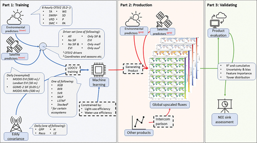
Figure 1. Study overview. The UFLUX framework includes three major parts. Part 1: tower-level upscaling model training. This part also considers factors affecting the upscaling performance by feeding with different parameter combinations. Part 2: producing upscaled GPP, Reco, NEE, H, and LE fluxes using the trained models. Upscaled estimates of NEE are produced from upscaled Reco and GPP (i.e. NEE = Reco – GPP), however we also validate this against directly upscaled NEE. Part 3: validating the upscaled models and products at both tower and global scales. Global NEE variability is also assessed using the upscaled products.

(1) $\mathit{F}=\mathit{f}\left(\mathit{RS},\mathit{Env},\mathit{Aux}.\right)$(1)

Typically, the predictors in upscaling studies are satellite remote sensing ($\mathit{RS}$) vegetation proxy products and environmental driver data $\left(\mathit{Env}\right)$ (Joiner and Yoshida 2021; Jung et al. 2020; Zeng et al. 2020). In addition, auxiliary parameters ($\mathit{Aux}.$) like geolocation and vegetation classification are commonly also taken into consideration (Joiner and Yoshida 2020; Jung et al. 2020; Zeng et al. 2020). The carbon and water fluxes were interconnected by the water-use efficiency (Hatfield and Dold 2019) – i.e. applying the interquartile ranges of light-use and water-use efficiencies derived from EC towers across ecosystem types into the machine learning models as constraints.

Machine learning algorithms are commonly used for flux upscaling (Reichstein et al. 2019) because they can well fit non-linear relations, e.g. light-use efficiency (Monteith 1972) (supplementary Section A.1. GPP upscaling theory), respiration-temperature responses (Lloyd and Taylor 1994), and the evapotranspiration rates (Penman 1948) (supplementary Section A.2. Reco, H, and LE upscaling theories). The machine learning algorithms were constrained by light-use and water-use efficiencies, resulting in a framework that is not purely data-driven but rather aligns more closely with ecological sensibility. The relationships fitted during the ‘training part’ are extrapolated to the globe in the ‘production part’ on daily 0.25° resolutions (Figure 1). In the final ‘validating part’, estimates are corroborated using the leave-one-out cross-validation (Marchetti 2021) approach (Figure 1).

2.2. Data

2.2.1. EC flux data

Daily EC data are selected from the 206 open-access FLUXNET2015 towers (Pastorello et al. 2020). We use NEE (NEE_VUT_REF), GPP (GPP_NT_VUT_REF), Reco (RECO_NT_VUT_REF) (Table S1) with data filtering criteria in line with Tramontana et al. (2016) and Joiner and Yoshida (2020). We use the daily values when 1) less than 33% of half-hourly data are gap-filled, 2) the NEE uncertainty is smaller than 3 g C m⁻² d⁻¹, and 3) the difference between daytime- and night-time partitioned GPP is smaller than 3 g C m⁻² d⁻¹. We also use H (H_F_MDS) and LE (LE_F_MDS) from the FLUXNET2015 database with data filter criteria referring to Jung et al. (2019) – we use the daily values with less than 33% of half-hourly data are gap-filled.

2.2.2. Predictor data

Predictor data include satellite vegetation proxies and climate reanalysis, which provides environmental drivers.

Here, we examine three widely used satellite vegetation proxies (supplementary Section B. Full data description): solar-induced chlorophyll fluorescence (SIF), near-infrared reflectance (NIRv), and enhanced vegetation index (EVI) are used. The SIF data (2007–2014) are from the 8-day downscaled (0.05^◦) GOME-2 (Global Ozone Monitoring Experiment-2) product (v2.0) were linearly interpolated to the daily scale (Duveiller et al. 2020). Both NIRv and EVI are taken from the daily 500-m nadir bidirectional reflectance distribution function (BRDF)-adjusted reflectance from moderate resolution imaging spectroradiometer (MODIS) (MCD43A4 V006) product (Huete et al. 1997; Schaaf and Wang 2015).

In accordance with the literature, the environmental drivers (supplementary Section B. Full data description) are obtained from a climate reanalysis database (Joiner and Yoshida 2020; Jung et al. 2020). In total eight environmental drivers are used from the Climate Forecast System Version 2 (CFSV2) of National Centers for Environmental Prediction (NECP) (Saha et al. 2014): temperature (2 m above ground, TA), downward shortwave radiation (at surface, SWIN), specific humidity (2 m above ground) for calculating vapour pressure deficit (VPD), soil moisture content (5 cm integral below surface, SWC), U-/V- wind components (10 m above ground) converted to wind speed (WS) and wind direction (WD), precipitation rate (at surface, P) and pressure (PA). All environmental drivers were resampled from 6-hourly to daily sum (P) or daily mean (TA, SWIN, VPD, SWC, U/V, WS, WD, and PA).

Considering the time coverage of different datasets – i.e. GOME-2 SIF data started in 2007, while the FLUXNET2015 database ended in 2014 – the time for training is from 2007 to 2014. To assess the predictive capacity of UFLUX in forecasting future fluxes, the global flux estimation was generated for a time frame extending from 2007 to 2018, surpassing 2014. In the context of time lag effects, we incorporated time lag considerations by integrating time stamps into the machine learning models.

2.3. UFLUX implementation and assessment

2.3.1. Model training and global estimation

In the training part, a complete model training (Figure 2) refers to a case described in Table 1. In line with the literature, the upscaling is implemented separately within each plant functional type from the International Geosphere Biosphere Programme (IGBP) (Joiner and Yoshida 2020; Jung et al. 2020; Zeng et al. 2020) using the leave-one-out cross validation (LOOCV) (Marchetti 2021). Specifically, the model is trained and tested per ecosystem type, e.g. only data with the same plant function type are used for training and testing the model. For a PFT group (PFT_i) containing m sites, for example, one site (site_j) is treated as the test set, and the rest of m-1 sites construct the training set. This process is repeated for each tower, so the algorithm is trained and tested 206 times in total (supplementary Section A.3. Data splitting rationale). In this way, we train the model in 17 cases (Table 1), and each case includes the 206 complete model training runs. Models trained in cases 0 to 4 are used for upscaling carbon, water, and energy fluxes. Please note that the upscaling setup (e.g. from algorithm) of cases 0 to 4 is the default uniform setup of UFLUX.

Figure 2. Schematic diagram of one complete upscaling model training. The red dashed arrows indicate the data flow into the machine-learning (ML) upscaling model. The orange blocks or oval are input data to models, green blocks are model output data, and blue blocks refer to components the models. The block on the bottom-left reveals the machine-learning model workflow. The block on the right shows the model scenarios: 1) spatial estimation (estimating the whole GPP time series at one EC tower by training the model using data at other towers with the same plant functional type); 2) temporal estimation (estimating future GPP from data in the past).

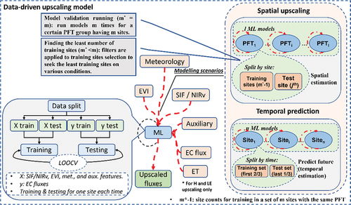
Table 1. All the testing cases in the study to comprehensively assess the influences from technical aspects on the upscaling performance. ‘High uncertainty’ in case 8 and 9 indicates EC towers where the testing upscaling performance is poor (R² < 0.3) in case 0. The different training setup between the base case and other cases is highlighted in orange.

	Flux	Algorithm	EVI	SIF/NIRv	Feature set	Training towers	Test towers
	Base case
Case 0	GPP	XGB	MODIS	SIF	All	All	All
	Testing for other fluxes
Case 1	Reco	XGB	MODIS	SIF	All	All	All
Case 2	NEE	XGB	MODIS	SIF	All	All	All
Case 3	H	XGB	MODIS	SIF	All	All	All
Case 4	LE	XGB	MODIS	SIF	All	All	All
	Testing machine learning algorithms
Case 5	GPP	RFR	MODIS	SIF	All	All	All
Case 6	GPP	MLP	MODIS	SIF	All	All	All
Case 7	GPP	SVR	MODIS	SIF	All	All	All
Case 8	GPP	LSTM	MODIS	SIF	All	All	High uncertainty
Case 9	GPP	Stacked	MODIS	SIF	All	All	High uncertainty
	Testing feature combinations
Case 10	GPP	XGB	MODIS	SIF	No SIF	All	All
Case 11	GPP	XGB	MODIS	SIF	No SIF & EVI	All	All
Case 12	GPP	XGB	MODIS	SIF	Only SIF & EVI	All	All
Case 13	GPP	XGB	MODIS	SIF	Only met.	All	All
Case 14	GPP	XGB	MODIS	SIF	Only aux.	All	All
	Testing NIRv
Case 15	GPP	XGB	MODIS	NIRv	All	All	All
	Testing the training space
Case 16	GPP	XGB	MODIS	SIF	All	Rand.^1	All

¹Rand.: randomly selected training towers with number ranging from one to all available towers.

In the production part, the trained upscaling models are applied to calculate fluxes across the globe from 2007 to 2018 on daily 0.25° resolutions. Unlike other flux types, NEE has two distinct pathways for upscaling. The first approach involves separately upscaling GPP and Reco on a global scale and then calculating NEE (denoted as ‘NEE_ind’). On the other hand, the second approach directly upscales NEE to the globe using EC measurements (denoted as ‘NEE_dir’). In this study, both pathways are considered for a thorough assessment of the UFLUX framework (supplementary Section A. Upscaling theories).

2.3.2. Assessment measures

We examine the UFLUX estimates by comparing them to EC fluxes based on the coefficient of determination (R²), linear regression slope, root mean squared error (RMSE), and mean bias error (MBE), and the uncertainty was measured using the interquartile range (IQR) of the MBE, following the methodology in our previous studies (Zhu et al. 2022; Zhu, McCalmont, et al. 2023). In addition to the technical testing, we also analyse the contribution of each predictor to the upscaling performance via the commonly used permutation feature importance (Altmann et al. 2010). It repetitively shuffles the column of each feature to corrupt the data and computes a reference score on the model fitted with the corrupted version of data. The score sum of all features equals one, and the importance of each feature can be evaluated thereby. Fluxes derived from UFLUX were compared with other EC upscaling products particularly to examine their ability to preserve certain key ecological parameters, e.g. the light-use efficiency, water-use efficiency, and Bowen ratio (Chapin, Matson, and Vitousek 2011).

2.4. Identify the factors restricting the upscaling effectiveness

2.4.1. Impacts of machine learning algorithms and predictors

To investigate the impacts of machine learning algorithms on the upscaling performance, we examine six machine learning algorithms (case 0 and case 5–9, Table 1) focusing on GPP: 1) Support vector regression (SVR) (Awad and Khanna 2015). 2) Random forest regression (RFR) (Breiman 2001). 3) Multi-layer perceptron neural networks (MLP) (Rumelhart, Hinton, and Williams 1986). 4) EXtreme Gradient Boosting (Xgboost, XGB) (Chen and Guestrin 2016). 5) Long short-term memory (LSTM) (Hochreiter and Schmidhuber 1997). 6) Stack of RFR, MLP, and XGB with a final regressor (Wolpert 1992). Hyperparameters of the machine learning algorithms were tuned automatically by exhaustively considering all parameter combinations via the grid search technique (Pedregosa et al. 2011). LSTM is a mainstream deep learning technique by effectively processing very long time series (Hochreiter and Schmidhuber 1997). Both LSTM and the stacked algorithm have the potential for improvements (Wolpert 1992), thereby they are only tested in areas where the upscaling accuracy tends to be less satisfactory, e.g. the tropics, and where the dominant plant functional type is evergreen broadleaf forest (Jung et al. 2020). The aim is to determine if the relatively poor upscaling performance in these areas can be addressed with an advanced and complicated algorithm architecture.

We also inspect how will the upscaling performance be affected by the combination of predictors (which are commonly referred to as features in machine learning studies) in case 0 versus case 10–14 (Table 1). By inter-comparing case 0 against case 15, we expect to investigate the possible difference using solar-induced fluorescence (SIF) and near-infrared reflectance (NIRv).

2.4.2. Impacts of EC spatial sampling

The spatial sampling of EC towers (i.e. the spatial density of the measurements) could introduce uncertainty in flux upscaling. We analyse the impacts of EC spatial sampling via a ‘similarity’ test – i.e. the ‘similarity’ between training and test sets in case 16 (Table 1). The fluxes, particularly carbon fluxes, are driven by or closely associated with environmental variables, specifically climate conditions and the vegetative greenness measured by satellite proxies. The ‘similarity’ was calculated by the coefficient of determination of these environmental variables between the target geolocations and those sampled with EC towers. In case 16, for a test EC tower, there are $\mathit{n}$ training towers with the same plant functional type. These $\mathit{n}$ towers construct a training sample space. In the $i^{\mathit{th}}$of $\mathit{n}$ tests, one randomly selects $\mathit{i}$ ($\mathit{i}\in \left[0,\mathit{n}\right]$) towers from the sample space to create a subspace for training and testing the machine learning model. The upscaling performance and the highest ‘similarity’ are recorded for the following analysis. In addition, we calculate the ‘similarity’ between geolocations of satellite pixels and corresponding EC towers, enabling us to apply this analysis globally.

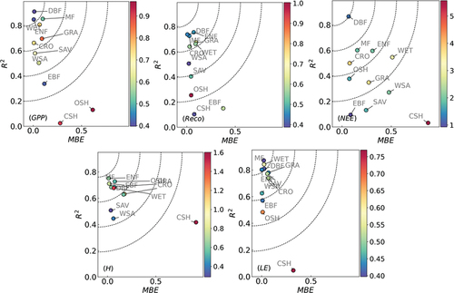
Figure 3. Upscaling performance for GPP, Reco, NEE, H, and LE at EC level. The x axis is normalised mean the bias error (MBE), the y axis is the R², and the colourmap indicates the normalised root mean squared error (RMSE). The normalised MBE and RMSE are corresponding values divided by the mean fluxes (e.g. normalised GPP MBE = GPP MBE/GPP), considering the different flux magnitude across Plant Functional Types (PFTs). The dots represent the averaged MBE and R² of PFTs: Mixed Forests (MF), Evergreen Needleleaf Forests (ENF), Grasslands (GRA), Woody Savannas (WSA), Savannas (SAV), Evergreen Broadleaf Forests (EBF), permanent Wetlands (WET), Deciduous Broadleaf Forests (DBF), Open Shrublands (OSH), Croplands (CRO), and Closed Shrublands (CSH). The dot colours of the four subplots separately represent PFT-averaged levels of GPP, Reco, H, and LE fluxes derived from EC. The contours represent how well the upscaling performance is considering both the R² and MBE. The dot curves are for better visual effects in distinguishing the upscaling performance between plant function types.

3. Results

3.1. UFLUX validations

In this section, we will present the tower-level UFLUX upscaling performance for GPP, Reco, H, and LE fluxes as well as their global distribution. Furthermore, directly and indirectly upscaled NEE will be compared. Seasonal variability of all the five fluxes is also demonstrated.

The R² and MBE distribution of all ecosystem classes concentrated on the upper left region of Figure 4, i.e. higher R² but smaller MBE absolute values. For PFTs with low R², the MBE tends to be small too – e.g. GPP of evergreen broadleaf forests (EBF). The median R² and MBE were 0.72 and 0.02 g C m⁻² d⁻¹ for GPP, were 0.61 and 0.14 g C m⁻² d⁻¹ for Reco, were 0.68 and −1.49 W m⁻² for H and were 0.76 and 0.2 W m⁻² for LE (Table 2). The R² value on average of the four fluxes was 0.7. Closed shrublands had the lowest performance among plant functional types for GPP, H, and LE, whilst evergreen broadleaf forests had the lowest performance for Reco (Figure 4). The upscaling performance seemed uncorrelated with flux strength, for example, closed shrublands (CSH) had medium GPP strength compared with other plant functional types.

Figure 4. UFLUX upscaling performance in terms of R² and MBE at the cross-validation eddy covariance towers. The MBE unit for GPP and Reco is g C m⁻² d⁻¹ and for H and LE is W m⁻².

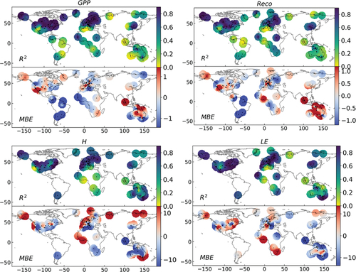
Table 2. Statistical metrics of the UFLUX upscaling performance at FLUXNET2015 towers using SIF as the satellite vegetation proxy, the unit for RMSE and MBE are g C m⁻² d⁻¹ for GPP and Reco and W m⁻² for H and LE. See table S2 for the results of using MODIS NIRv as the satellite vegetation proxy.

	R^2	Slope	RMSE	MBE
GPP
Min	0	−0.25	0.48	−5.16
Q1	0.43	0.43	1.26	−0.66
Median	0.72	0.72	1.77	0.02
Mean	0.63	0.7	2.07	0.01
Q3	0.87	0.91	2.52	0.61
Max	0.97	1.87	6.75	4.92
Reco
Min	0	−0.12	0.25	−7.68
Q1	0.35	0.4	0.88	−0.58
Median	0.64	0.66	1.34	0.14
Mean	0.57	0.7	1.69	0.14
Q3	0.8	0.93	1.98	0.66
Max	0.96	2.96	8.58	7.55
H
Min	0.01	−0.14	7.19	−38.46
Q1	0.54	0.44	14.19	−8.8
Median	0.68	0.64	18.68	−1.49
Mean	0.61	0.62	21.57	−1.19
Q3	0.78	0.8	24.13	5.97
Max	0.91	1.43	60.34	48.74
LE
Min	0.03	−0.25	5.49	−83.52
Q1	0.57	0.56	11.85	−6.67
Median	0.76	0.71	16.2	0.2
Mean	0.67	0.71	19.61	−1
Q3	0.86	0.89	23.47	6.56
Max	0.98	2.17	100.89	33.28

The Northern Hemisphere, where 82% of the EC towers are located (Schimel et al. 2015), had the highest R² and the smallest MBE absolute valuesin particular, Europe and North America where EC towers were densely located. Africa and South America have fewer EC towers, lower R² and larger MBE absolute values than the Northern Hemisphere (Figure 4).

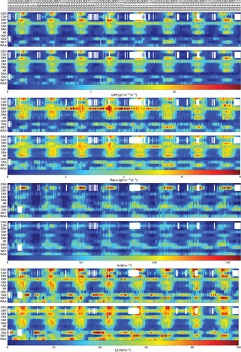
Overall, the UFLUX estimates displayed patterns that aligned with EC measurements, albeit with less intensity (Figure 5). This difference in flux intensity was particularly observed in evergreen broad forest (EBF) for Reco and closed shrublands (CSH) for H. For example, large Reco fluxes between 2008 and 2011 in EBF were barely seen in UFLUX estimates (Figure 5).

Figure 5. Fingerprints for measured and estimated fluxes averaged by PFTs for GPP, Reco, H, and LE, respectively. Their x-axes represent the time dimension, their y-axes represent PFTs, and the colour indicates the flux strength. For each flux of GPP, Reco, H, and LE, the upper fingerprint plot shows the measured fluxes, and the bottom fingerprint shows the estimated fluxes.

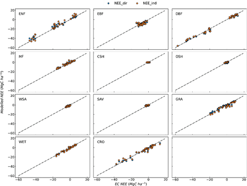
The scatters of EC NEE against UFLUX NEE are distributed close to the one-to-one line across ecosystem types (Figure 6). The direct and indirect estimates of NEE showed a high degree of similarity in their distribution, with an R² value close to 0.8. On the global scale, the annual difference between EC NEE and UFLUX NEE estimates was smaller 3 Mg C ha⁻¹. Please refer to Figure S1 and S2 for the interannual variability of UFLUX carbon fluxes including NEE and UFLUX NEE multi-year cumulative variations, respectively.

Figure 6. Scatters of EC NEE against UFLUX NEE estimates for both direct estimates (Nee_dir, blue dots) and indirect estimates (Nee_ind, orange dots).

3.2. Seasonal variability of global estimates

For carbon fluxes, according to Figure 7, GPP and Reco contain expected seasonal and regional patterns. Higher annual GPP and Reco were seen in South America, Central Africa, and Southeast Asia and no obvious seasonal variations were observed in these regions. Northeast America and Eurasia were found with much stronger seasonality: higher values in the summer, while lower values in the winter. Regarding NEE, India, West Asia and Northeast America were the main carbon sources (i.e. positive NEE), while Central Africa, West America, Europe, and Southeast Asia were the main carbon sinks. South America and Central Africa were the main carbon sinks annually. Whilst North America and Eurasia turned from carbon sinks to sources in September and vice versa in May.

Figure 7. Multi-year averaged monthly upscaled GPP, Reco, NEE, H, and LE fluxes.

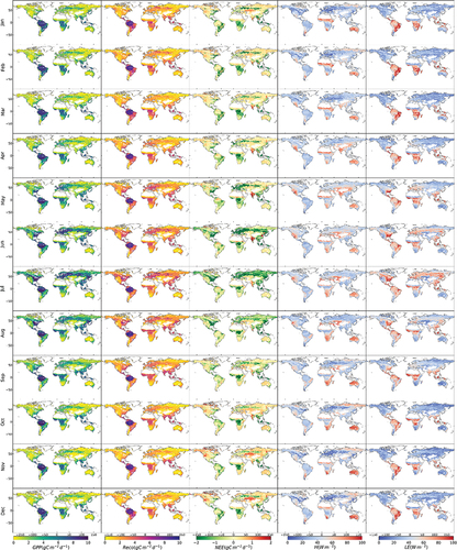
In terms of energy and water fluxes, Northwest America, South Africa, Middle East and Australia were seen with higher H. Whilst Northeast America, South America, Central Africa, and Southeast Asia were seen with higher LE. Like carbon fluxes, both H and LE were observed with expected patterns – i.e. higher values in the summer and were observed with lower values in the winter (Figure 7). Please see Figure S3 for the annual maps of UFLUX GPP, Reco, NEE, H, LE from 2001 to 2021.

3.3. Impacts of algorithms and predictors on the flux upscaling

Considering the effects of machine-learning algorithms, R² of XGB and RFR were consistently higher than SVR, and MLP across ecosystems and the interquartile range (IQR) of both R² and MBE were smaller for XGB and RFR than for SVR and MLP (Figure 8 and Table 3). The model running time of validating at FLUXNET2015 towers for XGB, RFR, SVR, and MLP were 15, 36,415 and 17 min. The performance of using XGB (median R²: 0.72 and MBE IQR: 1.27 g C m⁻² d⁻¹) was close to using RFR (median R²: 0.63 and MBE IQR: 1.4 g C m⁻² d⁻¹) for flux upscaling at a daily scale (Figure 8 and Table 3). In contrast, SVR (R²: 0.3 and MBE IQR: 2.72 g C m⁻² d⁻¹) and MLP (R²: 0.5 and MBE IQR: 4.2 g C m⁻² d⁻¹) showed relatively poor performance.

Figure 8. Inter-comparison of the data-drive GPP upscaling performance using xgboost (XGB), Random Forest Regression (RFR), support vector Regression (SVR), and multiple Layer perceptron (MLP) across 11 plant functional types.

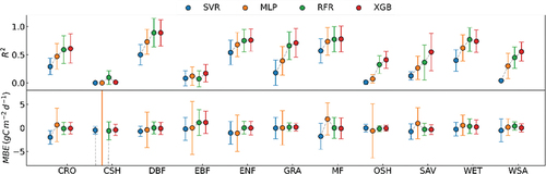
Table 3. The median values of statistical metrics of the upscaling performance using random forest regression, support vector regression and multiple Layer perceptron at FLUXNET2015 towers; the unit for RMSE and MBE is g C m⁻² d⁻¹. See table S3 for the full table.

	R^2	Slope	RMSE	MBE
RFR	0.63	0.67	2.05	0.08
SVR	0.3	0.16	3.11	−0.81
MLP	0.5	0.5	3.37	−0.06

In addition, in regions (e.g. tropics) where the UFLUX accuracy was low (median R²: 0.1), the R² of using LSTM (median R²: 0.13) and stacked machine learning (median R²: 0.09) were also very low (Table 4).

Table 4. The median values of statistical metrics of the upscaling performance using deep learning techniques at towers with poor performance using xgboost, the unit for RMSE and MBE are g C m⁻² d⁻¹ for GPP and Reco and W m⁻² for H and LE. See table S4 for the full table.

	R^2	Slope	RMSE	MBE
XGB	0.10	0.21	2.91	0.58
LSTM	0.13	0.19	2.52	0.40
Stacking	0.09	0.14	3.07	0.43

The feature importance – i.e. the score measures how useful the input features are at predicting fluxes – showed that SIF was the most important feature for GPP and LE upscaling (Figure 9(a)). Please see Figure S4 for feature importance results across plant functional types. The importance of SIF (59%) far exceeded EVI (10%), meteorology, and other auxiliary features. For Reco, VPD (19%), EVI (19%), and SIF (15%) contributed more than 50% of importance. It is noteworthy, that the contribution of air temperature (12%) was relatively less important for Reco upscaling. Solar radiation contributed 42% of importance in H upscaling, and the contribution of SIF and EVI was separately less than 6%. For LE upscaling, SIF was the most important features, with an importance of 45%.

Figure 9. (a) Importance of features of the data-driven machine learning model, values of only feature importance > 5% are shown in the figure. The sum of feature importance values equals 100%. For example, for GPP: satellite SIF (59.3%) and EVI (9.5%), meteorology solar radiation (rg, 5.7%), air temperature (Tair, 8.1%), and vapour pressure deficit (VPD, 3.0%), and other auxiliary ones, including day difference (DD, the days to the time-series beginning, 3.7%), day of year (DoY, 5.3%), Koppen climate classes (KOP., 4.8%), and – (not-effective, like longitude and latitude, 0.6%). (b) Upscaling model R² and MBE in six different feature combination scenarios: ‘all feat’. (i.e. all features, the benchmark scenario), ‘no SIF’ (i.e. dropping SIF from the features), ‘no SIF & EVI’ (i.e. dropping both SIF and EVI), ‘only SIF & EVI’ (i.e. dropping all other features except SIF and EVI), ‘only met’. (i.e. dropping all features except solar radiation (rg), air temperature (Tair), and vapour pressure deficit (VPD)), and ‘only aux’. (i.e. dropping SIF, EVI, Rg, Tair, and VPD).

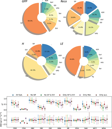
Regarding the effects of feature combinations, R² and MBE in upscaling of using six different feature combinations showed seemingly contradictory findings compared with the feature importance analysis. Small changes were seen in R² and MBE for most ecosystem classes when SIF or SIF & EVI were dropped from the features (Figure 9(b)). Interestingly, scenarios using only SIF and EVI as features achieved R² and MBE very close to scenario using all features in croplands and grasslands. In open shrublands and woody savannahs, R² of scenarios using SIF and EVI was much higher than scenario using all features. Scenarios using meteorology only achieved R² and MBE similar to scenario using all features in evergreen broadleaf forests, evergreen needleleaf forests, and wetlands. In deciduous broadleaf forests and mix forests, scenario using auxiliary features only achieved R² and MBE close to scenario using all features (Figure 9(b)).

The upscaling performance of using solar-induced fluorescence (SIF) and near-infrared reflectance (NIRv) was every close. In general, the R² of using SIF was marginally higher than that of using NIRv – e.g. – the median R² for GPP upscaling of using SIF (0.72) was 4% higher than using NIRv (0.69) (Table 5).

Table 5. The median values of statistical metrics of the upscaling performance using NIRv at FLUXNET2015 towers; the unit for RMSE and MBE are g C m⁻² d⁻¹ for GPP and Reco and W m⁻² for H and LE. See table S5 for the full table.

	R^2	Slope	RMSE	MBE
GPP	0.69	0.68	1.89	0.09
Reco	0.61	0.64	1.30	0.16
H	0.58	0.55	23.42	−0.97
LE	0.66	0.62	20.56	1.30

3.4. Impacts of EC spatial sampling on the flux upscaling

Overall, R² increased with more training towers while MBE decreased (Figure 10(a)).

Figure 10. Impacts on the upscaling performance from the EC towers per se. (a) Relationship between the training site number and the upscaling model performance in terms of R² and MBE. Colours represent the ‘similarity’ classes: low (less than 50% of the variance in the test site GPP can be explained by the training sites), medium (50% − 75% of the variance in the test site GPP can be explained by the training sites), and large (more than 75% of the variance in the test site GPP can be explained by the training sites). Note for this sub-figure, the upscaling mode for each site, that has k training sites, iteratively ran k! times. (b) The number of medium similarity towers for locations across the globe. White & khaki regions are in urgent need of more EC towers as the number of medium similarity towers smaller than three.

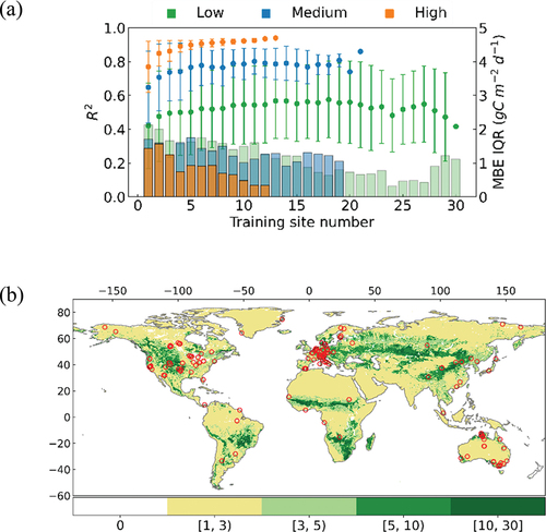
Regarding the relationship between similarity analysis and UFLUX upscaling performance, the highest level of similarity, i.e. the highest R² in satellite vegetation proxy time series between the test EC tower and a training tower, showed a strong positive linear correlation (slope = 0.92, intercept = 0.07, correlation coefficient = 0.82, and p-value = 0) with the R² of flux upscaling. The standard deviation of the similarity also showed a positive linear correlation with the up-scaling R² (slope = 2.90, intercept = 0.17, correlation coefficient = 0.67 and p-value = 0).

Regarding the training tower number and similarity level, for test towers with high- and/or medium-level similarity training towers, the R² IQR became narrower, while the number of training sites increased. The upscaling R² is kept around 0.85 or higher when the model was trained with at least one high similarity or five medium similarity sites. In contrast, even when the model was trained with more than 20 low-level similarity towers, the upscaling R² was still lower than 0.6. In the current FLUXNET2015 database, European and North American sites were seen with almost all the high and medium similarity sites, while sites in other regions were only seen with low similarity sites (Figure 10(b)). This distribution pattern was similar to the distribution of upscaling model performance – higher R² also clustered in Europe and North America. Please see Figure S5 for more information about the relationship between upscaling performance and the ‘similarity’ metric across biomes and EC towers.

3.5. Assessment on reproducing key ecological parameters

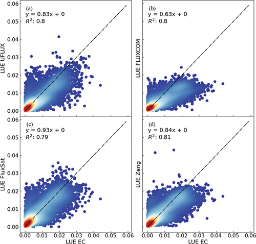
The UFLUX was compared alongside existing openly accessible EC upscaling products – i.e. FLUXCOM (Jung et al. 2020), FluxSat (Joiner and Yoshida 2021), and (Zeng et al. 2020) – in preserving the light-use efficiency. Considering the impacts of various spatial resolution across products, all the products were resampled into the same spatial resolution (0.5^◦) and then interpolated into the geolocations of EC towers. All the four products showed an R² of around 0.8 when compared with EC light-use efficiency. In terms of the linear regression slope, the FluxSat was 12% higher than UFLUX and Zeng of which the slope was around 0.83. In the meantime, the FLUXCOM was 24% smaller in slope (Figure 11).

Figure 11. Comparison of light-use efficiency (LUE) derived from eddy covariance (EC) towers and flux upscaling products, interpolated at the corresponding tower locations. Dot density in red regions signifies high values, contrasting with blue regions indicating lower values. Dashed lines represent the one-to-one relationship.

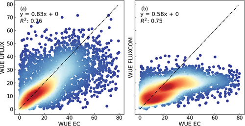
The efficacy of UFLUX was assessed in terms of preserving water-use efficiency in comparison to FLUXCOM (Jung et al. 2019), as FluxSat (Joiner and Yoshida 2021) solely provides GPP and (Zeng et al. 2020) exclusively supplies carbon-related fluxes (GPP, Reco, and NEE). UFLUX and FLUXCOM achieved equivalent R² of 0.75 when compared with EC water-use efficiency (Figure 12). The UFLUX had a higher linear regression slope of 0.83, and the slope for FLUXCOM was 0.58. A relatively small slope was particularly observed where the water-use efficiency was larger than 20 g C (Kg H₂O)⁻¹.

Figure 12. Comparison of water-use efficiency (WUE) derived from eddy covariance (EC) towers and flux upscaling products, interpolated at the corresponding tower locations. Dot density in red regions signifies high values, contrasting with blue regions indicating lower values. Dashed lines represent the one-to-one relationship. The water-use efficiency unit is g C (kg H₂O)⁻¹.

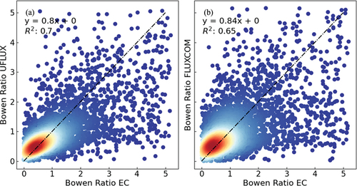
To further evaluate the ability of upscaled fluxes in representing the type of heat transfer, the UFLUX was compared with FLUXCOM in reproducing the Bowen ratio (Jung et al. 2019). In general, the results of UFLUX and FLUXCOM were comparable. The R² for UFLUX exceeded that of FLUXCOM by a marginal 0.05, whereas the linear regression slope for FLUXCOM surpassed that of UFLUX by 0.04 (Figure 13).

Figure 13. Comparison of Bowen ratio (H/LE) derived from eddy covariance (EC) towers and flux upscaling products, interpolated at the corresponding tower locations. Dot density in red regions signifies high values, contrasting with blue regions indicating lower values. Dashed lines represent the one-to-one relationship.

4. Discussion

4.1. The advantages and drawbacks of ULFUX

The UFLUX was suggested to hold great promise for providing uniform upscaling routines. Some previous studies that have examined the upscaling of carbon and water fluxes, often separately (Jung et al. 2019, 2020). However, this study represents a pioneering effort to upscale them together by interconnecting fluxes with key ecological parameters light-use and water-use fluxes. This holds significance, for example, the UFLUX preserved the ecosystem water-use efficiency and thereby can provide guidance on nature-based solutions (Zhu, Olde, et al. 2023). The UFLUX framework offers a means to disentangle whether the uncertainties stem from upscaling methodologies or the inherent characteristics of EC systems.

The UFLUX can capture approximately 70% of the variability of carbon, water, and energy fluxes (i.e. averaged R² = 0.7, Table 2), while the uncertainty in terms of interquartile range (IQR) was relatively small (1.5 g C m⁻² d⁻¹ for GPP and Reco, 15 W m⁻² for H and LE). The term ‘variability’ is derived from the study by Joiner and Yoshida (2020) and it pertains to the mean R² calculated across GPP, Reco, H, and LE fluxes – with NEE inferred as the difference between Reco and GPP. The UFLUX framework also exhibited great potential in predicting future fluxes (R² = 0.73, Table S6). Given its strong capability in capturing the non-linear relationship between fluxes and the environment, the UFLUX was expected to be beneficial for quantifying ecosystem light- and water-use efficiency, global carbon and water budgets, and further for climate goals (Smith et al. 2021). Directly and indirectly upscaled NEEs were both consistent with EC measurements, and the difference in the sum of nearly 10 years was smaller than 10 Mg C ha⁻¹ across ecosystems (Figure 6(a)). The spatial distribution of the upscaled NEE was in a great agreement with the literature (Jiang et al. 2022; Keenan and Williams 2018; Zeng et al. 2020).

It is particularly crucial to exercise caution when examining the interannual variability of the net ecosystem carbon exchange derived from any global estimates. To provide an illustration, the NEE trend described in Zeng et al. (2020) was not apparent in our observations of UFLUX NEE (Figure S1). Please also see the comparison of UFLUX against EC and other upscaling products in Figure S6. This discrepancy does not imply that UFLUX was superior or vice versa, but rather highlights the inherent constraints of data-driven approaches. The method UFLUX used to interconnect carbon and water fluxes exhibited improvements, particularly in tropical latent energy (Figure S6e) and water-use efficiency (Figure 12). However, these improvements are far from being enough, the UFLUX still underestimated the tower-level light-use and water-use efficiencies, as well as the Bowen ratio (Figures 11, 12, and Figure 13). The UFLUX still struggled to capture the interannual variability of fluxes in tropics (Figure S6). The ability to accurately capture the flux interannual variability depends on the efficacy of machine learning algorithms, the proficiency of satellite vegetation proxies in monitoring ecosystem (carbon) dynamics, and the representativeness of EC towers in sampling global terrestrial ecosystems (Aubinet, Vesala, and Papale 2012). For example, major carbon source sinks (e.g. South America and India in Figure 6(b)) have very limited number of EC towers (Pastorello et al. 2020; Schimel et al. 2015) and this added extra uncertainty in flux estimation. In this case, it would be very important to know the limiting factors and potential improvements for the upscaling performance, while standardizing the upscaling routine in a consistent and comparable manner.

The quantification of uncertainty presents a challenge when dealing with black-box models, such as machine-learning UFLUX, particularly in light of the heterogeneous spatial scales inherent in the flux footprints derived from tower-based observations, which serve as the basis for training these machine learning models. A potential strategy for addressing this challenge in non-MODIS-based data products may involve the exploration of geographically weighted regression (GWR). Our future research will be focused on the upscaling or estimation of spatiotemporal variations in uncertainty within the UFLUX framework (Joiner and Yoshida 2020).

4.2. Dominant factor(s) determining the upscaling performance

4.2.1. The limited impacts from algorithms and environmental drivers

The Xgboost algorithm is highly recommended for flux upscaling due to its superior performance compared to other machine learning algorithms commonly used for flux upscaling (Ichii et al. 2017; Joiner and Yoshida 2020). It achieved the highest R² values and the lowest level of uncertainty. Furthermore, it had a shorter running time and does not require extensive computational resources like graphics processing units (GPUs), which are typically used in deep learning techniques (Reichstein et al. 2019). This means that promoting the use of Xgboost would not incur significant financial costs, making it a more affordable option for countries with limited resources for flux quantification (Hill, Chocholek, and Clement 2017). Moreover, the reduced reliance on computational resources also minimizes the potential for additional carbon emissions, which have been observed in many deep learning applications (Strubell, Ganesh, and McCallum 2020). It is worth noting that the introduction of deep learning and stacked machine learning techniques did not yield substantial improvements in flux upscaling in regions like the tropics (Figure S7) where the upscaling performance was unsatisfactory and uncertainties in global carbon cycles were significant (Jung et al. 2020). This suggests that prioritizing technical advancements may not be the most crucial factor in accurately quantifying global fluxes.

The debate surrounding the effects of satellite vegetation proxies on upscaling performance continues. In agreement with the literature, it has been found that SIF provided the most significant information for flux upscaling (Guanter et al. 2012; Zhang et al. 2016). However, removing SIF or other satellite vegetation proxies has minimal impact on the upscaling performance (Figure 9(b)). Satellite vegetation proxies indicate the intensity of photosynthesis and/or the greenness of ecosystems, which are closely related to fluxes, particularly GPP intensity (Verrelst et al. 2015). Fluxes are influenced to a large extent by environmental factors such as solar radiation, air temperature, and vapour pressure deficit (Zhu et al. 2022). In addition, we explored the inclusion of carbon fluxes as a feature for model training to predict energy fluxes, and vice versa. However, our experimentation did not yield any substantial enhancements, as evidenced by a small change in R², which remained below 0.1. Considering the remarkable capabilities of machine learning algorithms in capturing non-linear relationships, it is possible that the role of satellite products as flux proxies could be replaced by combinations of environmental drivers. However, further investigation is necessary to determine the extent to which satellite vegetation proxies can be replaced by the combinations of environmental drivers. This is due to the intricate nature of the relationship between fluxes and environmental drivers. In many ecosystems, fluxes are predominantly influenced by solar radiation, air temperature, and vapour pressure, while in other ecosystems, factors such as water table depth exhibit a strong correlation with flux intensity (Zhu, McCalmont, et al. 2023). In such cases, the utilization of satellite vegetation proxies can offer substantial value.

4.2.2. The importance of sufficient EC sampling

The findings of this study indicate that the spatial sampling of EC towers plays a crucial role in the performance of flux upscaling. A model trained with data from a diverse range of towers that sampled various ecosystems tended to exhibit better upscaling performance (Figure 3 and Table S7). For instance, the upscaling performance was particularly strong for deciduous broadleaf forests and evergreen needleleaf forests, which had 21 and 31 towers, respectively, with long-term data records out of a total of 206 FLUXNET2015 towers (Pastorello et al. 2020). On the other hand, the upscaling performance was poorer for evergreen broadleaf forests (13 towers) and shrublands (9 towers), with data records covering a limited period of time (Pastorello et al. 2020). For example, five out of six South American towers had time series lengths shorter than four years, and four of those towers had time series shorter than two years (Figure S8) (Pastorello et al. 2020). It is worth noting that the diversity in the representation of EC towers is also significant. Despite 70 out of 206 FLUXNET towers being located in Europe, nearly 50% of the towers were deployed in forests, while grasslands and croplands, which constitute 39% of Europe’s land cover, had less than 9% and 16% of towers, respectively (https://www.eea.europa.eu/themes/agriculture/intro). The extant towers were prone to be present in regions with relatively higher vegetation coverage (Figure S8). Additionally, the specific characteristics of ecosystems pose challenges in flux upscaling. For instance, the GPP time series for evergreen broadleaf forests tend to be relatively stable (Jung et al. 2020), making it more difficult to accurately estimate fluxes compared to ecosystems with strong seasonal variations. Nevertheless, ensuring an evenly distributed network of EC towers would greatly benefit flux upscaling efforts (Sulkava et al. 2011).

When discussing the impacts of EC sampling on the flux upscaling performance, it is noteworthy that the choice of a method for partitioning data into training and test sets holds significant importance. Here, we employed the leave-one-out cross-validation (LOOCV) technique, akin to the approach employed in Joiner and Yoshida (2020). In this way, each tower played a role in the training and validation process. However, it is crucial to note that during individual validation steps (e.g. one of the 206 validations conducted for GPP), the specific tower under consideration remained entirely ‘untouched’. The rationale behind selecting this approach lies in the fact that, if we were to adopt the conventional data shuffle-split validation method (Pedregosa et al. 2011), data originating from the same tower could be utilized both for training and validation purposes. This contradicts our objective of spatially upscaling EC fluxes. The leave-one-out cross-validation method ensures a comprehensive validation process that guards against potential biases arising from selecting only subsets of towers for either training or validation purposes. This approach thus enhances the integrity and robustness of our validation procedures.

In the context of temporal analysis, we employed this methodology to assess the efficacy of upscaling techniques in predicting future fluxes. This entailed training the model using historical data to make future predictions. It is noteworthy that we refrained from employing a random selection approach for approximately two-thirds of the data, as such a method might inadvertently involve training models with data from ‘yesterday’ and ‘tomorrow’ to predict values for ‘today’. Under such conditions, the performance of linear regression would remain relatively stable. Therefore, we conducted an evaluation of machine learning algorithms in their capacity to forecast extended time series.

In contrast, we employed the conventional random data selection (Ichii et al. 2017; Pedregosa et al. 2011; Tramontana et al. 2016) for both spatial and temporal upscaling. For instance, the coefficient of determination (R²) for both aspects approached 0.75 for GPP, showing a slight improvement compared to the data splitting approach we currently employ, but it is suggested to choose a data selection/split method that suits the aim of study.

5. Summary and recommendations

This study standardizes the routine of upscaling EC fluxes, while also determining the key factors that affect the performance of upscaling. The UFLUX upscaling framework recommends the use of the Xgboost algorithm due to its relatively high accuracy (R² = 0.7 on a daily basis) and small uncertainties (1.5 g C m⁻² d⁻¹ for GPP and Reco, 15 W m⁻² for H and LE). Additionally, the UFLUX framework exhibited agreement in estimating NEE through direct and indirect upscaling pathways. Despite the advancements in machine learning algorithms, they did not significantly improve the upscaling performance. Among the predictors, SIF contributed the most information (ca. 50% of the contribution) to the upscaling model. Combining vegetation indices and environmental drivers can achieve similar results. The spatial sampling of EC towers plays a crucial role in flux upscaling, requiring at least three towers to achieve an upscaling R² of 0.75. The satellite vegetation proxies at these three towers should closely match the proxies at the target location, with an R² ranging between 0.5 and 0.75. If one tower can explain more than 75% of the variability in satellite vegetation proxies, it is sufficient to train the model and estimate the flux with this tower for the target location with an R² of 0.8. However, if less than 50% of the variability can be explained, no matter how many towers are used, it will not be enough. This study emphasizes the importance of a spatiotemporally even distribution of EC towers for reliable estimation of global fluxes.

Acknowledgements

The authors thank the FLUXNET research group for providing the CC-BY-4.0 (Tier one) open-access EC data (https://fluxnet.org/login/?redirect_to=/data/download-data/) and other research groups for providing open-access satellite and meteorology data. They also thank scikit-learn (https://scikit-learn.org/s table/install.html) team Xgboost (https://xgboost.readthedocs.io/en/stable/) for the packages that help with the implementation and validation for gap-filling approaches. SZ would like to acknowledge a Shell funded PhD studentship, and TQ’s contribution was supported by the NERC National Centre for Earth Observation (NE/X006328/1).

Disclosure statement

No potential conflict of interest was reported by the author(s).

Supplemental data

Supplemental data for this article can be accessed online at https://doi.org/10.1080/01431161.2024.2312266.

Additional information

Funding

This work was supported by the NERC National Centre for Earth Observation NE/X006328/1.

References

- Ai, J., G. Jia, H. E. Epstein, H. Wang, A. Zhang, and Y. Hu. 2018. “MODIS-Based Estimates of Global Terrestrial Ecosystem Respiration.” Journal of Geophysical Research: Biogeosciences 123 (2): 326–352. https://doi.org/10.1002/2017JG004107.
- Altmann, A., L. Toloşi, O. Sander, and T. Lengauer. 2010. “Permutation importance: a corrected feature importance measure.” Bioinformatics 26 (10): 1340–1347. https://doi.org/10.1093/bioinformatics/btq134.
- Aubinet, M., T. Vesala, and D. Papale. 2012. Eddy Covariance: A Practical Guide to Measurement and Data Analysis. Salmon Tower Building New York City USA: Springer Science & Business Media.
- Awad, M., and R. Khanna. 2015. “Support Vector Regression.” In Efficient Learning Machines, 67–80. Salmon Tower Building New York City USA: Springer.
- Badgley, G., L. D. L. Anderegg, J. A. Berry, and C. B. Field. 2019. “Terrestrial Gross Primary Production: Using NIRV to Scale from Site to Globe.” Global Change Biology 25 (11): 3731–3740. https://doi.org/10.1111/gcb.14729.
- Baldocchi, D. D. 2020. “How Eddy Covariance Flux Measurements Have Contributed to Our Understanding of Global Change Biology.” Global Change Biology 26 (1): 242–260. https://doi.org/10.1111/gcb.14807.
- Baldocchi, D., E. Falge, L. Gu, R. Olson, D. Hollinger, S. Running, P. Anthoni, et al. 2001. “FLUXNET: A New Tool to Study the Temporal and Spatial Variability of Ecosystem–Scale Carbon Dioxide, Water Vapor, and Energy Flux Densities.” Bulletin of the American Meteorological Society 82 (11): 2415–2434. https://doi.org/10.1175/1520-0477(2001)082<2415:FANTTS>2.3.CO;2.
- Beer, C., M. Reichstein, E. Tomelleri, P. Ciais, M. Jung, N. Carvalhais, C. Rödenbeck, et al. 2010. “Terrestrial Gross Carbon Dioxide Uptake: Global Distribution and Covariation with Climate.” Science 329 (5993): 834–838. https://doi.org/10.1126/science.1184984.
- Breiman, L. 2001. “Random Forests.” Machine Learning 45 (1): 5–32. https://doi.org/10.1023/A:1010933404324.
- Chapin, F. S., III, P. A. Matson, and P. Vitousek. 2011. Principles of Terrestrial Ecosystem Ecology. Salmon Tower Building New York City USA: Springer Science & Business Media.
- Chen, T., and C. Guestrin 2016. Xgboost: A Scalable Tree Boosting System. In: Proceedings of the 22nd acm sigkdd international conference on knowledge discovery and data mining, San Francisco California USA. pp 785–794.
- Dong, J., L. Li, Y. Li, and Q. Yu. 2022. “Inter-Comparisons of Mean, Trend and Interannual Variability of Global Terrestrial Gross Primary Production Retrieved from Remote Sensing Approach.” Science of the Total Environment 822:153343. https://doi.org/10.1016/j.scitotenv.2022.153343.
- Duveiller, G., F. Filipponi, S. Walther, P. Köhler, C. Frankenberg, L. Guanter, A. Cescatti, et al. 2020. “A Spatially Downscaled Sun-Induced Fluorescence Global Product for Enhanced Monitoring of Vegetation Productivity.” Earth System Science Data 12 (2): 1101–1116. https://doi.org/10.5194/essd-12-1101-2020.
- Fisher, R. A., and C. D. Koven. 2020. “Perspectives on the Future of Land Surface Models and the Challenges of Representing Complex Terrestrial Systems.” Journal of Advances in Modeling Earth Systems 12 (4): e2018MS001453. https://doi.org/10.1029/2018MS001453.
- Fu, Z., P. Ciais, I. C. Prentice, P. Gentine, D. Makowski, A. Bastos, X. Luo, et al. 2022. “Atmospheric Dryness Reduces Photosynthesis Along a Large Range of Soil Water Deficits.” Nature Communications 13 (1): 1–10. https://doi.org/10.1038/s41467-022-28652-7.
- Guanter, L., C. Bacour, A. Schneider, I. Aben, T. A. van Kempen, F. Maignan, C. Retscher, et al. 2021. “The TROPOSIF Global Sun-Induced Fluorescence Dataset from the Sentinel-5P TROPOMI Mission.” Earth System Science Data 13 (11): 5423–5440. https://doi.org/10.5194/essd-13-5423-2021.
- Guanter, L., C. Frankenberg, A. Dudhia, P. E. Lewis, J. Gómez-Dans, A. Kuze, H. Suto, et al. 2012. “Retrieval and Global Assessment of Terrestrial Chlorophyll Fluorescence from GOSAT Space Measurements.” Remote Sensing of Environment 121:236–251. https://doi.org/10.1016/j.rse.2012.02.006.
- Hatfield, J. L., and C. Dold. 2019. “Water-Use Efficiency: Advances and Challenges in a Changing Climate.” Frontiers in Plant Science 10:103. https://doi.org/10.3389/fpls.2019.00103.
- Hill, T., M. Chocholek, and R. Clement. 2017. “The Case for Increasing the Statistical Power of Eddy Covariance Ecosystem Studies: Why, Where and How?” Global Change Biology 23 (6): 2154–2165. https://doi.org/10.1111/gcb.13547.
- Hochreiter, S., and J. Schmidhuber. 1997. “Long Short-Term Memory.” Neural Computation 9 (8): 1735–1780. https://doi.org/10.1162/neco.1997.9.8.1735.
- Huete, A., H. Liu, K. Batchily, and W. Van Leeuwen. 1997. “A Comparison of Vegetation Indices Over a Global Set of TM Images for EOS-MODIS.” Remote Sensing of Environment 59 (3): 440–451. https://doi.org/10.1016/S0034-4257(96)00112-5.
- Ichii, K., M. Ueyama, M. Kondo, N. Saigusa, J. Kim, M. C. Alberto, J. Ardö, et al. 2017. “New Data-Driven Estimation of Terrestrial CO2 Fluxes in Asia Using a Standardized Database of Eddy Covariance Measurements, Remote Sensing Data, and Support Vector Regression.” Journal of Geophysical Research: Biogeosciences 122 (4): 767–795. https://doi.org/10.1002/2016JG003640.
- Jiang, F., W. Ju, W. He, M. Wu, H. Wang, J. Wang, M. Jia, et al. 2022. “A 10-Year Global Monthly Averaged Terrestrial Net Ecosystem Exchange Dataset Inferred from the ACOS GOSAT V9 XCO 2 Retrievals (GCAS2021).” Earth System Science Data 14 (7): 3013–3037. https://doi.org/10.5194/essd-14-3013-2022.
- Joiner, J., and Y. Yoshida. 2020. “Satellite-Based Reflectances Capture Large Fraction of Variability in Global Gross Primary Production (GPP) at Weekly Time Scales.” Agricultural and Forest Meteorology 291:108092. https://doi.org/10.1016/j.agrformet.2020.108092.
- Joiner, J., and Y. Yoshida. 2021. Global MODIS and FLUXNET-Derived Daily Gross Primary Production, V2. Oak Ridge, Tennessee, USA: ORNL DAAC.
- Jung, M., S. Koirala, U. Weber, K. Ichii, F. Gans, G. Camps-Valls, D. Papale, et al. 2019. “The FLUXCOM Ensemble of Global Land-Atmosphere Energy Fluxes.” Scientific Data 6 (1): 74. https://doi.org/10.1038/s41597-019-0076-8.
- Jung, M., M. Reichstein, C. R. Schwalm, C. Huntingford, S. Sitch, A. Ahlström, A. Arneth, et al. 2017. “Compensatory Water Effects Link Yearly Global Land CO 2 Sink Changes to Temperature.” Nature 541 (7638): 516–520. https://doi.org/10.1038/nature20780.
- Jung, M., C. Schwalm, M. Migliavacca, S. Walther, G. Camps-Valls, S. Koirala, P. Anthoni, et al. 2020. “Scaling Carbon Fluxes from Eddy Covariance Sites to Globe: Synthesis and Evaluation of the FLUXCOM Approach.” Biogeosciences 17 (5): 1343–1365. https://doi.org/10.5194/bg-17-1343-2020.
- Keenan, T., and C. Williams. 2018. “The Terrestrial Carbon Sink.” Annual Review of Environment and Resources 43 (1): 219–243. https://doi.org/10.1146/annurev-environ-102017-030204.
- Liu, X., L. Liu, J. Hu, J. Guo, and S. Du. 2020. “Improving the Potential of Red SIF for Estimating GPP by Downscaling from the Canopy Level to the Photosystem Level.” Agricultural and Forest Meteorology 281:107846. https://doi.org/10.1016/j.agrformet.2019.107846.
- Lloyd, J., and J. Taylor. 1994. “On the Temperature Dependence of Soil Respiration.” Functional Ecology 8 (3): 315–323. https://doi.org/10.2307/2389824.
- Marchetti, F. 2021. “The Extension of Rippa’s Algorithm Beyond LOOCV.” Applied Mathematics Letters 120:107262. https://doi.org/10.1016/j.aml.2021.107262.
- Monteith, J. L. 1972. “Solar Radiation and Productivity in Tropical Ecosystems.” The Journal of Applied Ecology 9 (3): 747–766. https://doi.org/10.2307/2401901.
- Papale, D., T. A. Black, N. Carvalhais, A. Cescatti, J. Chen, M. Jung, G. Kiely, et al. 2015. “Effect of Spatial Sampling from European Flux Towers for Estimating Carbon and Water Fluxes with Artificial Neural Networks.” Journal of Geophysical Research: Biogeosciences 120 (10): 1941–1957. https://doi.org/10.1002/2015JG002997.
- Pastorello, G., C. Trotta, E. Canfora, H. Chu, D. Christianson, Y.-W. Cheah, C. Poindexter, et al. 2020. “The FLUXNET2015 Dataset and the ONEFlux Processing Pipeline for Eddy Covariance Data.” Scientific Data 7 (1): 1–27. https://doi.org/10.1038/s41597-020-0534-3.
- Pedregosa, F., G. Varoquaux, A. Gramfort, M. Blondel, P. Prettenhofer, R. Weiss, V. Dubourg, et al. 2011. “Scikit-Learn: Machine Learning in Python.” The Journal of Machine Learning Research 12: 2825–2830. https://www.jmlr.org/papers/volume12/pedregosa11a/pedregosa11a.pdf.
- Penman, H. L. 1948. “Natural Evaporation from Open Water, Bare Soil and Grass.” Proceedings of the Royal Society of London. Series A. Mathematical and Physical Sciences 193:120–145.
- Reichstein, M., M. Bahn, M. D. Mahecha, J. Kattge, and D. D. Baldocchi, 2014. “Linking Plant and Ecosystem Functional Biogeography.” Proceedings of the National Academy of Sciences 111:13697–13702
- Reichstein, M., G. Camps-Valls, B. Stevens, M. Jung, J. Denzler, N. Carvalhais, and F. Prabhat. 2019. “Deep Learning and Process Understanding for Data-Driven Earth System Science.” Nature 566 (7743): 195–204. https://doi.org/10.1038/s41586-019-0912-1.
- Rumelhart, D. E., G. E. Hinton, and R. J. Williams. 1986. “Learning Representations by Back-Propagating Errors.” Nature 323 (6088): 533–536. https://doi.org/10.1038/323533a0.
- Saha, S., S. Moorthi, X. Wu, J. Wang, S. Nadiga, P. Tripp, D. Behringer, et al. 2014. “The NCEP Climate Forecast System Version 2.” Journal of Climate 27 (6): 2185–2208. https://doi.org/10.1175/JCLI-D-12-00823.1.
- Schaaf, C., and Z. Wang. 2015. “MCD43A3: MODIS. Terra and Aqua BRDF/Albedo.” Daily L3 Global 500.
- Schimel, D., R. Pavlick, J. B. Fisher, G. P. Asner, S. Saatchi, P. Townsend, C. Miller, et al. 2015. “Observing Terrestrial Ecosystems and the Carbon Cycle from Space.” Global Change Biology 21 (5): 1762–1776. https://doi.org/10.1111/gcb.12822.
- Slevin, D. 2016. “Investigating Sources of Uncertainty Associated with the JULES Land Surface Model.” The University of Edinburgh [Ph.D. thesis]. https://era.ed.ac.uk/handle/1842/20953?show=full.
- Smith, P., L. Beaumont, C. J. Bernacchi, M. Byrne, W. Cheung, R. T. Conant, F. Cotrufo, et al. 2021. “Essential Outcomes for COP26.” Global Change Biology 28 (1): 1–3. https://doi.org/10.1111/gcb.15926.
- Strubell, E., A. Ganesh, and A. McCallum. 2020. “Energy and Policy Considerations for Modern Deep Learning Research.” Proceedings of the AAAI Conference on Artificial Intelligence 34 (09): 13693–13696. https://doi.org/10.1609/aaai.v34i09.7123.
- Sulkava, M., S. Luyssaert, S. Zaehle, and D. Papale. 2011. “Assessing and Improving the Representativeness of Monitoring Networks: The European Flux Tower Network Example.” Journal of Geophysical Research: Biogeosciences 116. https://doi.org/10.1029/2010JG001562.
- Sun, Y., C. Frankenberg, M. Jung, J. Joiner, L. Guanter, P. Köhler, T. Magney, et al. 2018. “Overview of Solar-Induced Chlorophyll Fluorescence (SIF) from the Orbiting Carbon Observatory-2: Retrieval, Cross-Mission Comparison, and Global Monitoring for GPP.” Remote Sensing of Environment 209:808–823. https://doi.org/10.1016/j.rse.2018.02.016.
- Tramontana, G., K. Ichii, G. Camps-Valls, E. Tomelleri, and D. Papale. 2015. “Uncertainty Analysis of Gross Primary Production Upscaling Using Random Forests, Remote Sensing and Eddy Covariance Data.” Remote Sensing of Environment 168:360–373. https://doi.org/10.1016/j.rse.2015.07.015.
- Tramontana, G., M. Jung, C. R. Schwalm, K. Ichii, G. Camps-Valls, B. Ráduly, M. Reichstein, et al. 2016. “Predicting Carbon Dioxide and Energy Fluxes Across Global FLUXNET Sites with Regression Algorithms.” Biogeosciences 13 (14): 4291–4313. https://doi.org/10.5194/bg-13-4291-2016.
- Ueyama, M., K. Ichii, H. Iwata, E. S. Euskirchen, D. Zona, A. V. Rocha, Y. Harazono, et al. 2013. “Upscaling Terrestrial Carbon Dioxide Fluxes in Alaska with Satellite Remote Sensing and Support Vector Regression.” Journal of Geophysical Research: Biogeosciences 118 (3): 1266–1281. https://doi.org/10.1002/jgrg.20095.
- Verrelst, J., J. P. Rivera, C. van der Tol, F. Magnani, G. Mohammed, and J. Moreno. 2015. “Global Sensitivity Analysis of the SCOPE Model: What Drives Simulated Canopy-Leaving Sun-Induced Fluorescence?” Remote Sensing of Environment 166:8–21. https://doi.org/10.1016/j.rse.2015.06.002.
- Wang, H., I. C. Prentice, T. F. Keenan, T. W. Davis, I. J. Wright, W. K. Cornwell, B. J. Evans, et al. 2017. “Towards a Universal Model for Carbon Dioxide Uptake by Plants.” Nature Plants 3 (9): 734–741. https://doi.org/10.1038/s41477-017-0006-8.
- Wang, L., H. Zhu, A. Lin, L. Zou, W. Qin, and Q. Du. 2017. “Evaluation of the Latest MODIS GPP Products Across Multiple Biomes Using Global Eddy Covariance Flux Data.” Remote Sensing 9 (5): 418. https://doi.org/10.3390/rs9050418.
- Wolpert, D. H. 1992. “Stacked Generalization.” Neural Networks 5 (2): 241–259. https://doi.org/10.1016/S0893-6080(05)80023-1.
- Yang, F., K. Ichii, M. A. White, H. Hashimoto, A. R. Michaelis, P. Votava, A.-X. Zhu, et al. 2007. “Developing a Continental-Scale Measure of Gross Primary Production by Combining MODIS and AmeriFlux Data Through Support Vector Machine Approach.” Remote Sensing of Environment 110 (1): 109–122. https://doi.org/10.1016/j.rse.2007.02.016.
- Zeng, J., T. Matsunaga, Z.-H. Tan, N. Saigusa, T. Shirai, Y. Tang, S. Peng, et al. 2020. “Global Terrestrial Carbon Fluxes of 1999–2019 Estimated by Upscaling Eddy Covariance Data with a Random Forest.” Scientific Data 7 (1): 1–11. https://doi.org/10.1038/s41597-020-00653-5.
- Zhang, Y., X. Xiao, C. Jin, J. Dong, S. Zhou, P. Wagle, J. Joiner, et al. 2016. “Consistency Between Sun-Induced Chlorophyll Fluorescence and Gross Primary Production of Vegetation in North America.” Remote Sensing of Environment 183:154–169. https://doi.org/10.1016/j.rse.2016.05.015.
- Zhu, S., R. Clement, J. McCalmont, C. A. Davies, and T. Hill. 2022. “Stable Gap-Filling for Longer Eddy Covariance Data Gaps: A Globally Validated Machine-Learning Approach for Carbon Dioxide, Water, and Energy Fluxes.” Agricultural and Forest Meteorology 314:108777. https://doi.org/10.1016/j.agrformet.2021.108777.
- Zhu, S., J. McCalmont, L. M. Cardenas, A. M. Cunliffe, L. Olde, C. Signori-Müller, M. E. Litvak, et al. 2023. “Gap-Filling Carbon Dioxide, Water, Energy, and Methane Fluxes in Challenging Ecosystems: Comparing Between Methods, Drivers, and Gap-Lengths.” Agricultural and Forest Meteorology 332:109365. https://doi.org/10.1016/j.agrformet.2023.109365.
- Zhu, S., L. Olde, K. Lewis, T. Quaife, L. Cardenas, N. Loick, J. Xu, et al. 2023. “Eddy Covariance Fluxes Over Managed Ecosystems Extrapolated to Field Scales at Fine Spatial Resolutions.” Agricultural and Forest Meteorology 342:109675. https://doi.org/10.1016/j.agrformet.2023.109675.