Approaches and Techniques for Modelling CO₂ Emissions from Road Transport

Abstract

Transport accounts for around a quarter of CO₂ emissions globally. Transport modelling provides a useful means to explore the dynamics, scale and magnitude of transport-related emissions. This paper explores the modelling tools available for analysing the emissions of CO₂ from transport. Covering a range of techniques from transport microsimulation to global techno-economic models, this review provides insights into the various advantages and shortcomings of these tools. The paper also examines the value of having a broad range of perspectives for analysing emissions from transport. The paper concludes by suggesting that the broad range of models creates a rich environment for exploring a spectrum of policy questions around the emissions from transport, and the potential for combining modelling approaches further enhances the understanding that can be attained.

Keywords:

• CO₂ emissions
• transport models
• sustainability
• road transport

Introduction

The emission of greenhouse gases (GHGs) and the consequential climate change impacts is one of the greatest challenges facing the global community (Stern, 2007). Of the GHGs causing climate change, CO₂ is the most significant and the transport sector accounts for around 25% of CO₂ emissions, although this varies by scale and location, with energy supply, business and the residential sector making up the rest (DECC, 2013; International Energy Agency, 2009). In order to combat rising CO₂ emissions, it is essential to have a clear understanding of the generation of emissions within the transport system. The transport system is defined in this work as the infrastructure facilitating the movement of people and goods. This can include the physical infrastructure, ICT and vehicles. The policy and regulatory environment is also included in the review of modelling approaches as an important aspect of the transport system. This paper focuses on emissions from road transport, predominantly passenger transport rather than freight specifically, although freight may be implicitly included within some of the modelling techniques reviewed.

Modelling transport is a key element of transport research, exploring a multitude of factors and situations at a range of scales to provide insights and understanding of the challenges that face the infrastructure and the stakeholders who manage the infrastructure (Hensher & Button, 2008). Motivations behind modelling are as numerous as the challenges, and include such factors as improving inefficiencies in networks and examining the potential traffic impacts of changes to infrastructure (Brömmelstroet & Bertolini, 2011; Gudmundsson, 2011), exploring socio-economic effects of transport (Wismans, Van Berkum, & Bliemer, 2011), understanding supply and demand for transport (Proost & Van Dender, 2011), as well as modelling air quality and emissions (Brand, Tran, & Anable, 2012; Samaras et al., 2012). The scale of transport modelling is also wide-ranging, from the micro-level modelling of a single intersection, or local road network, to the global transport system.

Transport modelling provides tools that inform the user about the system in question and should aid in planning and policy decisions (De Dios Ortúzar & Willumsen, 2011). In order to facilitate a transition to a sustainable transport system, the choices that are made now must take into account the necessary emission reductions to prevent dangerous climate change and meet emission reduction targets (Intergovernmental Panel on Climate Change, 2007). There are a range of challenges arising from the transport sector, not least environmental damage, and examination of these issues through the use of transport models can aid decision-makers in dealing with these challenges (De Dios Ortúzar & Willumsen, 2011).

There are many examples of how and where emissions from transport have been accounted for through modelling approaches. At the local scale, traffic network models can provide planners with information about the emission impacts of infrastructure decisions by predicting traffic flows and travel decision-making (Gudmundsson, 2011). There are also behavioural models (Stern & Richardson, 2005) that can provide additional insights into travel behaviour (Hensher, Rose, Leong, Tirachini, & Li, 2013) and the potential emission impacts of changes to infrastructure, such as the uptake of electric vehicles (EVs) (Shafiei, Thorkelsson, et al., 2012). At a global level, large-scale energy systems models (e.g. Kim, Edmonds, Lurz, Smith, & Wise, 2012) can provide information about the transport sector internationally. These can support understanding of the action that is required at the transnational level to mitigation emissions of CO₂ in order to prevent dangerous climate change and thereby inform policy at the international and national levels.

This paper will provide a review of the modelling approaches available for accounting for emissions of CO₂ from road transport, across different scales. Whilst previous work has reviewed transport modelling approaches, the quantification of emissions from transport in models has not been explicitly emphasised and this paper aims to address this gap. The paper will begin by providing an overview of the modelling approaches that are considered in this work and the reasons for their inclusion. The models will then be analysed and critiqued, with example packages and capabilities presented. A synthesis will be presented that draws together the understanding of the different approaches and techniques that have been presented in the preceding sections and offer proposals on the relative merits of these models. This is followed by some final conclusions.

Model Classification for Review

The following types of models are reviewed in this research:

• Traffic network models: microsimulation;

• Behavioural models;

• Agent-based modelling;

• System dynamics modelling;

• Techno-economic; and

• Integrated assessment models (IAMs).

This classification of models has been used to provide a broad perspective of the ways that the transport system can be modelled. The models have been classified as such because of the different techniques that are used within the approach or the spatial and temporal context of the model. There are a spectrum of geographical and temporal scales represented, from the local to the global and the near-term future to a forecasting horizon of 2100. Figure 1 shows the scales covered by the modelling approaches included in this paper. The models may have differing underlying epistemologies, yet they all have an ability to represent elements of the transport system. They are also able to examine similar policy questions, particularly the question of the scale of emissions from transport, despite their differing perspectives and geographical scope. The various modelling tools they contain may be used in different ways by a variety of practitioners in order to explore a range of transport-related challenges. It is therefore interesting to consider the relative advantages and shortcomings of the different types of model and the necessity for multiple approaches in modelling the transport sector.

Figure 1. Spatial and temporal scales for the models reviewed.

This review will examine these issues by seeking to answer the following questions:

1. Which techniques and tools are used to model transport systems?

2. How do these capture emissions from transport? and,

3. What are the advantages and disadvantages of the different approaches?

Systematic Review of Transport Modelling Approaches

Synthesis of Modelling Capabilities by Model Type

The models that have been included in the systematic review in Table 1 represent a spectrum of modelling approaches spanning the spatial and temporal scales that are shown in Figure 1. The example packages were selected as they are representative of the techniques used in modelling the transport system and demonstrate different approaches to quantifying emissions from road transport. The following section synthesises the findings from the table and draws insights into the advantages and disadvantages of the various approaches. The traffic network, behavioural and agent-based modelling approaches have been grouped together, as these represent the micro-scale approaches which deal with disaggregate and capture individuals' or vehicles' movements, choices and behaviours. These are followed by the system dynamic modelling approaches and the macro-scale techno-economic and IAMs. Examples of combining modelling approaches are also provided.

Table 1. Review of approaches for modelling emissions from road transport

Modelling approach	Example packages/studies	Elements of transport system captured	Underlying concepts	Emissions calculation
1. Traffic network models — microsimulation	• DRACULA (Dynamic Route Assignment Combining User Learning and microsimulAtion)	Captures movement of vehicles within a predefined traffic network	Microsimulation modelling is built on the principles of the four-stage trip model (De Dios Ortúzar & Willumsen, 2011). The four-stage model is as follows:	DRACULA: assumes that fuel consumption factors are constant for vehicles that are idling or decelerating and calculates fuel consumption for accelerating vehicles using Equation (1). This is then converted into CO2 under the assumption that fuel burnt is converted to CO2. This does not take into account alternatively fuelled vehicles
	• VISSIM	Aggregate data across the network for emissions, delays, travel time, etc.	1. Trip generation	VISSIM: requires an add-on to module ‘EnViVer Pro’ which imports vehicle data to calculate CO2 emissions in the study area and outputs a table and graph of this (PTV Group, 2015)
			2. Trip distribution
			3. Mode split
			4. Traffic assignment
			Built on the principles of car following and lane changing rules which determine how the vehicles interact by maintaining gaps between vehicles through algorithms for minimum gap acceptance (Gipps, 1981; Young & Weng, 2005)
2. Behavioural models	• Stern and Richardson (2005) process-oriented framework, see Figure 2	Captures greater detail about individual decision-making travel choices	Activity-based models explore the activities that necessitate mobility to understand levels of transport and generate a clearer picture about decision-making. Travel is seen a result of activities and behaviour	Quantifying levels of transport demand that can then result in calculation of emissions of CO2
3. Agent-based modelling	• MATSIM (Multi-Agent Transportation Simulator Toolbox)	Captures the dynamics of behaviour in the transport system, as for behavioural models above, captures more detail than just the trips that are made, but understands behaviour and motivation	Models behaviour through a series of heterogeneous agents	Coupled with an emissions model can deliver unique insights into travel behaviour and road transport emissions
				MATSIM itself does not calculate emissions from road transport. However, Hatzopoulou, Hao, and Miller (2011) combined outputs from MATSIM with MOBILE6.2 to calculate emissions
4. System dynamics	• ASTRA — Assessment of Road Transport Strategies (Rothengatter et al., 2000)	Can capture interactions and feedbacks within complex systems such as transport	System dynamic models are built on CLD and stock and flow relationships	ASTRA: Environment Sub-module calculates gaseous transport emissions. Figure 3 shows the structure of this calculation within the sub-module; it includes factors for cold start, hot emission factors, etc.
	• MARS — Metropolitan Activity Relocation Simulator (Research Centre for Transport Planning and Traffic Engineering, 2009)			MARS: Three separate equations calculate emissions from road transport, the first calculates emissions from specific cars using speed output from MARS, another, total CO2 for private cars using distance and number of trips from MARS outputs and one which calculates CO2 emissions from public transport
5. Techno-economic models	• Roadmap (International Council for Clean Transportation, 2012)	Capture large-scale dynamics of the transport system through the socio-economic changes that occur, using a top-down modelling approach	Draws on socio-economic characteristics and forecast changes to estimate transport demand and technological forecasts are used to develop emission factors that allow projections of future emissions to be established	Roadmap: Tank-to-wheel CO2 emissions are estimated based on energy consumption, calculated from vehicle km travelled (VKT), which is established using socio-economic indicators, and vehicle efficiency using the following equation:
	• World Energy Projection System Plus (WEPS+) (US Energy Information Administration [EIA], 2011)		Roadmap: runs over five-year time steps from 2000 to 2015
				Figure 4 also shows how the emission calculations are structured in roadmap
6. IAMs	• Global Change Assessment Model (GCAM) (Kim et al., 2012)	Large-scale modelling of economy and environment with a sub-module for transport, capturing technological change and environmental impact driven by socio-economic factors	Runs in time steps of 15 years from 2005 to 2095 and achieves regional equilibrium in the regional markets in each time step (Kyle & Kim, 2011)	Demand for transport is calculated in GCAM using Equation (1). Equation (2) calculates the costs of passenger transport modes and Equation (3) uses this to calculate mode share. These can then be coupled with emission factors to provide regional and global projections of emissions from transport

Traffic Network, Behavioural and Agent-Based Models

Traffic network models cover a range of scales, from macro to micro. This review has focused on microsimulation as it represents a key subset of these models. Transport demand is generated within microsimulation modelling as follows. An origin–destination (O–D) matrix is used with the models to represent individual trips within the network and in the traffic assignment part of the four-stage model (McNally, 2008). The network that underlies traffic models is constructed from real-world traffic networks using a series of ‘nodes’, ‘links’ and ‘zones’ (Willumsen, 2008). Nodes represent junctions and intersections whilst links are roads that connect nodes. The zones are areas between which (or within which) trips are made and from which the O–D matrix is constructed. For example, a trip will be from origin (O) — zone x, to destination (D) — zone y (Atkins-ITS, 2013). Further details on the behavioural rules that govern microsimulation of traffic can be found in the detailed manuals for the models (Liu, 2007; Verkehr, 2011). Table 1 summarises the general method for emissions calculation within microsimulation packages, whilst Equation (1) shows the calculation of fuel consumption in DRACULA, which is then used to calculate CO₂ emissions (Liu, 2005).

Calculation of fuel consumption in DRACULA:(1)

where f is the fuel consumption factor, v, the speed of the vehicle, a, the acceleration of the vehicle, and c₀ and c₁ are constants defined in Ferreira (1982).

For VISSIM, an additional add-on package, ‘EnViVer’ is required for the calculation of emissions (PTV Group, 2015). This package draws on the emission calculations developed in the VERSIT + model which uses the following equation to calculate traffic emissions for pollutant j (TE_j, g/hour):(2)

Where presents the predicted mean emission factor (g/km) for pollutant j, vehicle class k and speed-time profile l, TV_k,m presents the traffic volume with respect to vehicle class k (vehicles/hour) for a particular section of road m, where speed-time profile l would apply and L_m presents the length of road section m (km) (Smit, Smokers, Schoen, & Hensema, 2006, p. 17). This is used to calculate the emissions across a network simulation in VISSIM, accounting for different vehicle classes and the speed-time profile for each vehicle.

By understanding the levels of demand for mobility within the traffic system and according to the scenario under scrutiny, the level of emissions can be established and the impacts of policy changes analysed (Dowling, Holland, & Huang, 2002). There are a range of additional behavioural rules within microsimulation that are not identified in column 4 of Table 1 (‘Underlying concepts’) and details of these can be found in the individual model manuals (Liu, 2007; Verkehr, 2011). Overall, microsimulation provides a series of useful techniques for modelling emissions from road transport, as it allows small changes in the network to be analysed in terms of their impacts on transport and the resulting emissions.

One of the goals of behavioural research in transport is to understand how travellers use the transport infrastructure in order to better predict needs and enhance decision-making, thus providing a more holistic view of activities (Davidson et al., 2007; Stern & Richardson, 2005). Behavioural models draw heavily on the disciplines of social psychology and behavioural economics for the underlying principles and frameworks (Schaap & van de Riet, 2012). Stern and Richardson (2005) present a ‘process-oriented framework’ for understanding travel behaviour, as shown in Figure 2. This shows how additional factors beyond the need to travel from an origin to a destination can be considered in understanding travel behaviour, including factors such as the motivation for travel, scheduling and any constraints on travel.

Figure 2. Process-oriented framework of the behaviour of road users.

Source: Adapted from Stern and Richardson (2005)

Activity-based models focus on the underlying motivations behind travel decisions, allowing travel patterns to be more clearly understood and to quantify the demands on the mobility system (Axhausen & Gärling, 1992; McNally & Rindt, 2008). By quantifying the amount of travel within a network through an activity-based approach, emission factors can be applied to estimate the emissions of CO₂ from road transport.

Agent-based models have been used in activity-based approaches, but there are also elements of agent-based modelling principles incorporated within some microsimulation models. Agent-based modelling characterises a series of agents within a practice space, the modelled world in which the agents interact, in order to understand behavioural dynamics (Köhler et al., 2009). Agents have behaviours and interact with other agents and their environment, which can alter their behaviour and this provides insights into the dynamics of the system being modelled (Macal & North, 2010). These approaches have been used in the social and biological sciences to understand behaviour (Grimm et al., 2006) and there are examples of their use in transport, including Köhler et al. (2009), Quadstone Paramics (2013) and Shafiei, Stefansson, Asgeirsson, Davidsdottir, and Raberto (2012). There are also examples of the inclusion of agent-based modelling principles in traffic microsimulation models. PARAMICS is a traffic network model that characterises pedestrian activities and pedestrian traffic interactions, thereby incorporating an agent-based modelling approach (Quadstone Paramics, 2013). In addition, qualitative methods and virtual reality approaches outlined by Dougherty, Fox, Cullip, and Boero (2000) are areas that have the potential to increase the degree of agency within traffic network simulation. An additional advantage of using agent-based modelling to explore systems such as those found in the transport sector is that a series of ‘heterogeneous agents’ can be modelled. These allow detailed insights into the interactions in the system and a ‘bottom-up’ approach to be taken (Garcia, 2005; Shafiei, Stefansson, et al., 2012).

MATSIM captures the dynamics of the transport system with a behavioural-oriented approach, characterising this through agents within a traffic network. The MATSIM programme itself does not calculate road transport emissions, but a study by Hatzopoulou et al. (2011) coupled MATSIM with the MOBILE6.2 model to estimate the emissions generated by the travel behaviour being modelled. MOBILE6.2 uses fuel economy outputs to calculate emissions of CO₂, but these are not varied for speed and engine type, as the calculations for other pollutants in MOBILE6.2 are; however a wide range of vehicle types are accounted for within the model and the addition of the CO₂ calculation was new for version 6.2 (US EPA, 2003).

A different use of agent-based modelling is seen in a study by Shafiei, Thorkelsson, et al. (2012) where an agent-based modelling approach is applied to explore uptake of EVs. They used a Multinomial Logit model to characterise car purchase decisions and analyse the willingness of agents to consider an EV over a conventional Internal Combustion Engine. The model also allowed a study of the extent to which exposure to information affects willingness to consider the alternatives. The data requirements of this approach lie in the parameters for characterisation of the agents. The model outputs information about the market share of EVs over the scenario period. Shafiei, Thorkelsson, et al. (2012) demonstrate the application of agent-based modelling approaches to the transport sector and their ability to capture behavioural dynamics in the market. Whilst this modelling approach does not output direct emission calculations from road transport, it provides a useful insight into the fuel mix of the future vehicle fleet. This is useful in understanding future emissions from road transport and the extent to which emission reduction targets might be met by uptake of alternatively fuelled vehicles.

System Dynamics

Fishwick (2007) describes a dynamic model as one which captures the way a system changes in time and this type of approach has been used across a range of disciplines in the physical and social sciences. System dynamic models are based around causal loop diagrams (CLD) that simulate and analyse relationships and mathematical modelling of stocks and flows (Sternman, 2000). They incorporate both qualitative and quantitative techniques and analysis, making them highly versatile tools (Pfaffenbichler, Emberger, & Shepherd, 2010). Shafiei, Stefansson, et al. (2012) describe system dynamics modelling of complex systems as a “top-down approach that looks at the process of market developments as a whole and facilitates understanding the interactions of many stakeholders … ” (Shafiei, Stefansson, et al., 2012, p. 45).

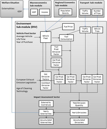
CLD are the main technique used within system dynamics modelling to explore the qualitative relationships between different aspects of the system. They work by identifying entities, which are the aspects of the system that can affect other aspects and can be affected by others, and they must represent an unspecified quantity. There are also exogenous factors within system dynamics that are predefined constants interacting with the identified entities. These entities are then connected by directional causal links, which form the loops that are reinforcing or balancing, representing positive or negative feedbacks within the system, see Pfaffenbichler (2011) for more details. System dynamics has been applied in transport because the feedback and linkages these models are able to capture are useful for identifying interactions within the transport system. Shepherd (2014) provides a review of the ways that system dynamics modelling has been used to capture the transport system. Figure 3 shows the environment sub-module in ASTRA which is responsible for the calculation of CO₂ emissions. The vehicle fleet in the model is driven by socio-economic factors and this is coupled with the transport sub-module to calculate fuel consumption which is used to calculate the in use emissions. Upstream-embodied emissions in the fuel production and vehicle production are also accounted for in calculating the total emissions from the activity in the model (Rothengatter et al., 2000).

Figure 3. ASTRA environment sub-module.

Source: Adapted from Rothengatter et al. (2000)

The calculation of CO ₂ emissions in MARS is undertaken using Equation (3) (Pfaffenbichler, 2003).(3) where is the specific carbon dioxide emissions of the mode car for a trip from i to j in year t (g/Vh km), the average speed for a car trip from i to j in year t depending on the applied policy instrument vector output of MARS (km/h), and the parameters, source MEET project (Samaras & Ntziachristos, 1998).

This demonstrates how the outputs from the trip model in MARS are used to calculate emissions of CO₂ by applying an emission factor, based on average speed, to the vehicle km outputs (Pfaffenbichler, 2003). The emission factors are drawn from the MEET project (Samaras & Ntziachristos, 1998). These are then aggregated up through the MARS model to produce total emissions generated by specific modes of transport within the system being modelled.

MARS and ASTRA are selected as examples of system dynamic modelling in transport because they show how the techniques can be applied at the city and regional scales, respectively. These modelling approaches are highly effective at capturing complex dynamics at a larger geographical and temporal scale than the behavioural models, which incorporate different factors into the calculation of CO₂ emissions from road transport. It is clear from the selection of these two models as examples of system dynamic approaches that they are versatile tools. For example, the calculations made in ASTRA account for upstream emissions embodied in the vehicle and fuel production, where the MARS model does not. This will lead to variations in the outputs for emissions from road transport; in some cases, the inclusion of upstream emissions may be seen as more accurate in accounting for total emissions from transport; however, there may be policy questions that just address the tank-to-wheel emissions, and the inclusion of upstream emissions may distort results in these cases. The selection of the most appropriate tool must be considered with the specific policy or research questions being examined.

Techno-economic Models

Techno-economic models include a range of tools that look at the relationships between technology, the economy and the wider impacts of this and can also be combined with socio-economic data (Anable, Brand, Tran, & Eyre, 2012). E3 models are a subset of this category and capture the interactions between energy, economy and the environment. These models tend to be macro-scale models, sometimes looking at transport only as a sub-sector of wider economic activity (Schafer, 2012). They have the ability to deliver insights into sector-level emissions and generally provide aggregate outputs. As with many macro-scale models, the details captured in traffic models or behavioural approaches are often overlooked, but there are examples of attempts to integrate some of this detail into these approaches.

Figure 4 shows the process for calculating emissions in the ICCT Roadmap model, a techno-economic model of the transport system. It uses socio-economic indicators coupled with vehicle and fuel technology projections to estimate the emissions from road transport into the future, through the process shown in Figure 4.

Figure 4. Simplified emission calculation in Roadmap.

Source: Adapted from International Council for Clean Transportation (2012)

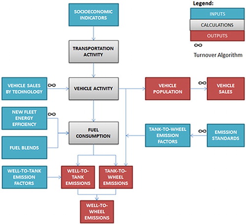
Figure 5. Outputs from Roadmap for global WTW transport CO _2e emissions to 2050.

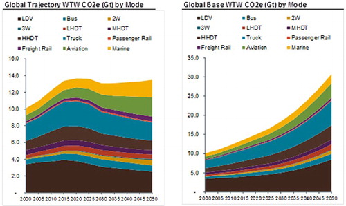
Figure 5 shows an example of the outputs from the Roadmap model. On the right-hand side of the figure is a base-case scenario for global well to wheel (WTW) CO_2e emissions to 2030. The left-had side has been subjected to a policy trajectory by adjusting the parameters shows in Figure 4. Outputs can also be delivered for specific modes or regions. This demonstrates the value that this kind of model can have in understanding macro patterns of emissions, future projections and modal share, as well as providing insights into regional responsibilities, which can be used at the international policy-making level.

IMACLIM-R is a hybrid dynamic equilibrium model that explores emissions from the transport sector for 2001–2100 (Waisman, Guivarch, & Lecocq, 2013). The model characterises transport emissions as based on four factors:

• Technological

  1. Intensity of fuels

  2. Energy intensity of mobility

• Behavioural

  1. Modal structure

  2. Volume of mobility

The model captures non-energy and non-price drivers of transport dynamics as a bridge between top-down and bottom-up modelling approaches. The model includes specific features for rebound effects, induced traffic, modal breakdowns and impacts of land-use decisions (Waisman et al., 2013).

An example of E3 modelling of transport is given within the US Energy Information Administration's (EIA) (2011) WEPS+. Within WEPS+, the Transportation Sector Model (ITRAN) captures the transport sector. The model is a large-scale model that provides aggregate sector emission projections. These outputs are based on socio-economic activity, GDP and population figures in a macroeconomic model, and fuel prices from the refinery/electricity models. Outputs from the model include service demand in passenger miles by sub-mode, fuel and region, and service intensity in passenger miles per Btu by sub-mode, fuel and region (US EIA, 2011).

These models are providing aggregate emission projections for the transport system which are at a large spatial scale. Unlike the micro-scale approaches, individuals or vehicle dynamics are not apparent, but the insights can be useful for national and international policy- and decision-making. In particular, demonstrating the magnitude and geographical distribution of emissions can proportion responsibility for those emissions and the need for delivery of emission reduction measures.

Integrated Assessment Models

IAMs can be used to model the interactions between the economy and the environment across the entire system in order to understand long-term changes and processes at the macro scale. They are able to capture the transport sector as a component of economic activity and some models allow the running of sectoral modules independently. They are similar in scale and scope to techno-economic models, however they are designed to further explore the environmental changes associated with the economy.

The GCAM is an open licensed IAM (Kim et al., 2012). It is a partial equilibrium model which allows the separate areas of the economy to be modelled independently. It is a large-scale model that produces aggregate emission projections, but the transport module can deliver insights into future technological pathways and mode shares for the global regions (Kim et al., 2012). Equations (4)–(6) show how emissions from transport are calculated in GCAM (Kyle & Kim, 2011):

Demand for passenger transport in region r and time period t, D_rt, is calculated using the following:(4)

where σ is the base year (2005) calibration parameter, Y, the GDP per capita, P, the total service price aggregated across all modes, N, population, α, the income elasticity, and β, the price elasticity.

Total cost of any passenger mode (P_i) in region r and time period t is calculated using the following:(5)

where FP is the fuel price, I, the vehicle fuel intensity, NFP, the vehicle non-fuel price, LF, the load factor, W, the wage rate and S, the vehicle speed.

Market share of a given mode S_i is calculated as follows:(6)

where SW is the share weight, P_i, the cost of transport service from above, λ, the cost distribution parameter and n, the number of modes.

These equations demonstrate how emissions from road transport are calculated within the IAM, GCAM. As is the case with techno-economic approaches, aggregate outputs concerning emissions from transport are produced from this type of model. Additional changes in technology, load factors and modal share can also be captured, and the impacts on emissions from the transport sector be analysed. These aggregate outputs are useful for policy- and decision-making at the national and international levels.

Combining Modelling Approaches

Combining multiple modelling techniques and approaches can deliver a new perspective of the transport sector or generate new understanding of the dimensions of the transport system (e.g. Köhler et al., 2009; Samaras et al., 2012; Shafiei, Stefansson, et al., 2012). As Shafiei, Stefansson, et al. (2012) suggest, “The real world problems in the transportation system, however, do not match up well with a single modelling approach” (p. 43).

Examples of combining models to create new approaches for understanding the transport system include Köhler et al. (2009) and Shafiei, Stefansson, et al. (2012) who combined agent-based and system dynamics techniques to explore transitions for sustainable mobility. Combining these two approaches allowed the exploration of behavioural interactions amongst heterogeneous agents in the agent-based modelling study components. The agent-based modelling components are then interfaced with a systems dynamics tool to explore how these behaviours play out in interactions and relationships in a future transition to sustainable mobility. As a further example of model combination, Samaras et al. (2012) combined a traffic network model with a model of ICT applications in transport to look at the emission implications arising from the integration of ICT in transport. This combination of multiple tools allowed the exploration of emissions from new ICT-enabled transport schemes that was otherwise challenging within the scope of a single modelling approach.

The EU GHG-TransPoRD project combined a series of modelling approaches to look at regional emissions from transport and understand trajectories for emission reductions in the transport sector (Fiorello et al., 2012; Schade & Krail, 2012). The research integrates three regional models including ASTRA, POLES (Prospective Outlook for the Long Term Energy System), TREMOVE and the metropolitan-scale MARS model to deliver greater understanding of potential emissions of GHGs at the EU scale towards 2050 (Fiorello et al., 2012). This combining of multiple approaches, including system dynamics modelling, can deliver insights into the complex interconnections of the international transport sector at this scale and meet the challenges of long-term forecasting of emission reductions.

The use of integrated models within a single research study allows some of the shortcomings of individual modelling techniques to be overcome. For example, combining focused behavioural studies with broader models such as traffic network models or system dynamics tools allows the understanding of individuals' mobility behaviour to be placed in the wider context. This supports delivery of outputs that can then be utilised by planners and decision-makers in policy development, although the integration of multiple modelling approaches can result in models which are more complex and may be challenging to non-expert users.

Summary

The previous sections have presented a range of approaches to modelling the transport system, and in particular the emissions of CO₂ from that system. Microsimulation, behavioural modelling and agent-based models all represent transport networks at the micro scale, characterising network-level interactions and the decisions that generate patterns of mobility. They are predominantly of value for the local-level decision-making as they can deliver insights into the geographical and temporal scales required for these decisions. These models vary in the level of detail captured about the individual, for example, microsimulation models capture the emissions from individual vehicles, but the dynamics of behaviour and motivations behind activities are not captured, whereas the agent-based and behavioural models capture greater details about these factors. The calculation of CO₂ emissions within these models varies, from applying an emission factor to the sum of travel demand generated to the more detailed calculations undertaken in VISSIM, with the add-on EnViVer Pro, which accounts for varying speed-time profiles and other factors that might affect the emissions (Smit et al., 2006). The applicability of an individual approach depends on the question being asked, with greater disaggregation generating more data, and perhaps the simplest approach for the questions is necessary, and often policy questions only require high-level aggregate emission estimates to understand the impacts of changes.

Techno-economic models and IAMs, however, allow insights at the scale of the regional or global economy, which can provide useful decision-making at the national and international policy-making levels (Paltsev et al., 2005). The quantification of emissions of CO₂ from road transport is necessary at both local and global levels and across the geographic and temporal scales in order that decisions can be effectively made that will mitigate emissions of CO₂ and avoid dangerous climate change. There are cases where the models are taken out of their conventional scales. For example, the EU TransTools model uses traffic network modelling principles to represent trips in Europe, providing a large volume of detail across a wide spatial area (Brun & Hansen, 2009). However, the general trend in transport modelling is for high levels of disaggregation when exploring a smaller spatial scale, with increasing computational demand, for example, in microsimulation tools or behavioural-type studies (Wegener, 2011). Figure 1 provides a graphical demonstration of the temporal and geographical spread of the models that have been reviewed in this paper, showing different approaches.

System dynamics modelling in transport is positioned between the small-scale microsimulation studies and the large-scale techno-economic models. For example, MARS examines dynamics in the transport system and the metropolitan scale, while ASTRA encompasses the European transport network. As suggested by Figure 1, this provides a set of tools that can project future transport systems at a scale which sits between micro-scale approaches and the large techno-economic models. Additional advantages of utilising the system dynamics approach are the capturing of feedback loops through the CLD diagrams which can capture the dynamics of multiple stakeholders and policy outcomes in a complex system (Shepherd, 2014). Particular areas of strength in system dynamics modelling of transport lie in the use of tools to capture interactions between land-use and transport, for example, MARS, and model of the markets for alternative vehicles, for example, Shepherd, Bonsall, and Harrison (2012). In terms of emissions, this can deliver insights in to the volume of emissions from the transport system under analysis, and the modelling of future vehicle markets yields insights into the potential for reduction in emissions of CO₂ from the vehicle fleet through uptake of alternative vehicles.

It is clear that whatever system scale the study requires, modelling tools are available that can provide insights into the transport challenges and the impacts of potential policies and solutions. In addition, the combining of multiple modelling techniques can deliver additional innovative approaches to modelling transport (Shafiei, Stefansson, et al., 2012).

Conclusions

Three research questions have underpinned this review of how transport models estimate the emissions generated by the transport system. The first was concerned with identifying the primary techniques and tools used to model transport systems. A classification of six main types has resulted, that is, microsimulation, behavioural, agent-based system dynamics, techno-economic and IAMs. The rationale behind the classification was the scope addressed by the model, that is, in terms of geographic, temporal and aggregation scale. In addition, the potential to interface and integrate models has been described.

The second research question concerned the methods used by the models to capture emissions from transport. This aspect of the research is synthesised in column 5 of Table 1. Essentially, each modelling approach implies some assumptions ranging from driver behaviour, vehicle market share, fuel consumption converting to CO₂ or to aggregate demand for transport on a broad scale. The efficacy of each type of model in capturing emissions overall rests on two broad sets of assumptions. The first assumptions are those underlying the way in which the model represents the transport system. The second assumptions underpin the detailed algorithms and emission factors that are then used to produce emission estimates. Whilst the first set are broadly understood and well reported, the second set of assumptions is often provided in more detailed manuals and aimed at an expert user. The overall efficacy of the model in each case will clearly rest on the appropriateness of both sets of assumptions to the context in which emissions are to be estimated.

The final research question was concerned with reflecting on the advantages and disadvantages of the different approaches. From the summary provided for each type of model, it is clear that each has advantages when used in the context (geographic, level of aggregation, etc.) for which it was designed and disadvantages occur when their use is extended beyond that original context. The practice of interfacing or integrating models has arisen, at least in part, from a need to fill some of the gaps in modelling capability that are still apparent in estimating emissions at particular geographic or temporal scales.

Clearly, the availability of different modelling tools makes the selection of the correct tool for the specific analysis important. Overall, different modelling perspectives and paradigms create a rich and diverse series of tools and techniques that can capture the transport system and resulting emissions. These form a highly valuable resource in a field where technology, economics, behaviour and other factors are all key to understanding the dynamics and the resulting emissions from the sector. In addition, combining different modelling approaches can deliver further insights and understanding of the emissions from transport, as often a single approach cannot fully capture the dynamics of such a complex system.

This review has outlined the ways in which transport models can capture emissions from the sector, the different approaches and techniques, and discussed the value of these. By focusing on the quantification of emissions in transport modelling, this paper contributes to the substantive body of literature on transport modelling whilst providing a novel perspective, with potential value to the academic and practitioner communities.

Disclosure Statement

No potential conflict of interest was reported by the authors.

Additional information

Funding

This work was supported by the Engineering and Physical Sciences Research Council [DTC ENERGY: Technologies for a low carbon future, Grant no. EP/G036608/1].

References

- Anable, J., Brand, C., Tran, M., & Eyre, N. (2012). Modelling transport energy demand: A socio-technical approach. Energy Policy, 41, 125–138. doi: 10.1016/j.enpol.2010.08.020
- Atkins-ITS. (2013). SATURN manual. Retrieved from http://www.saturnsoftware.co.uk/saturnmanual/chapters.html: Atkins and Institute for Transport Studies
- Axhausen, K. W., & Gärling, T. (1992). Activity-based approaches to travel analysis: Conceptual frameworks, models, and research problems. Transport Reviews, 12, 323–341. doi: 10.1080/01441649208716826
- Brand, C., Tran, M., & Anable, J. (2012). The UK transport carbon model: An integrated life cycle approach to explore low carbon futures. Energy Policy, 41, 107–124. doi: 10.1016/j.enpol.2010.08.019
- Brömmelstroet, M. T., & Bertolini, L. (2011). The role of transport-related models in urban planning practice. Transport Reviews, 31, 139–143. doi: 10.1080/01441647.2010.541295
- Brun, B., & Hansen, S. (2009). TRANS-TOOLS user guide version 2.0. Seville: EC Joint Research Centre.
- Davidson, W., Donnelly, R., Vovsha, P., Freedman, J., Ruegg, S., Hicks, J., … Picado, R. (2007). Synthesis of first practices and operational research approaches in activity-based travel demand modeling. Transportation Research Part A: Policy and Practice, 41, 464–488.
- DECC. 2013. 2012 UK greenhouse gas emissions, provisional figures. UK greenhouse gas emissions statistics. London: Author.
- De Dios Ortúzar, J., & Willumsen, L. G. (2011). Modelling transport. Chichester: Wiley.
- Dougherty, M., Fox, K., Cullip, M., & Boero, M. (2000). Technological advances that impact on microsimulation modelling. Transport Reviews, 20, 145–171. doi: 10.1080/014416400295220
- Dowling, R., Holland, J., & Huang, A. (2002). Guidelines for applying traffic microsimulation modelling software. Oakland, CA: Dowling Associates and California Department of Transportation.
- Ferreira, L. (1982). Car fuel consumption in urban traffic: The results of a survey in Leeds using instrumented vehicles (Working Paper No. 162). Leeds: Institute of Transport Studies, University of Leeds.
- Fiorello, D., Schade, W., Akkermans, L., Krail, M., Schade, B., & Shepherd, S. P. (2012). Results of the technoeconomic analysis of the R&D and transport policy packages for the time horizons 2020 and 2050. In GHG-TransPoRD (Reducing greenhouse-gas emissions of transport beyond 2020: Linking R&D, transport policies and reduction targets). Milan: European Commission.
- Fishwick, P. (2007). Handbook of dynamic system modelling. London: Chapman & Hall.
- Garcia, R. (2005). Uses of agent-based modeling in innovation/new product development research*. Journal of Product Innovation Management, 22, 380–398. doi: 10.1111/j.1540-5885.2005.00136.x
- Gipps, P. G. (1981). A behavioural car-following model for computer simulation. Transportation Research Part B: Methodological, 15, 105–111. doi: 10.1016/0191-2615(81)90037-0
- Grimm, V., Berger, U., Bastiansen, F., Eliassen, S., Ginot, V., Giske, J., … Deangelis, D. L. (2006). A standard protocol for describing individual-based and agent-based models. Ecological Modelling, 198, 115–126. doi: 10.1016/j.ecolmodel.2006.04.023
- Gudmundsson, H. (2011). Analysing models as a knowledge technology in transport planning. Transport Reviews, 31, 145–159. doi: 10.1080/01441647.2010.532884
- Hatzopoulou, M., Hao, J., & Miller, E. (2011). Simulating the impacts of household travel on greenhouse gas emissions, urban air quality, and population exposure. Transportation, 38, 871–887. doi: 10.1007/s11116-011-9362-9
- Hensher, D. A., & Button, K. J. (2008). Handbook of transport modelling. Oxford: Elsevier.
- Hensher, D. A., Rose, J. M., Leong, W., Tirachini, A., & Li, Z. (2013). Choosing public transport — incorporating Richer behavioural elements in modal choice models. Transport Reviews, 33, 92–106. doi: 10.1080/01441647.2012.760671
- Intergovernmental Panel on Climate Change. (2007). Technical summary. In S. Solomon, D. Qin, M. Manning, Z. Chen, M. Marquis, K. B. Averyt, … H. L. Miller (Eds.), Climate change 2007: The physical science basis. Contribution of Working Group I to the Fourth Assessment Report of the Intergovernmental Panel on Climate Change (pp. 19–91). Cambridge: Cambridge University Press.
- International Council for Clean Transportation. (2012). Global transportation roadmap — model documentation and user guide. San Francisco: Author.
- International Energy Agency. 2009. Transport energy and CO2: Moving towards sustainability. Paris: OECD.
- Kim, S. H., Edmonds, J., Lurz, J., Smith, S. J., & Wise, M. (2012). The ObjECTS framework for integrated assessment: Hybrid modeling of transportation. The Energy Journal, (Special Issue 2), 63–92.
- Köhler, J., Whitmarsh, L., Nykvist, B., Schilperoord, M., Bergman, N., & Haxeltine, A. (2009). A transitions model for sustainable mobility. Ecological Economics, 68, 2985–2995. doi: 10.1016/j.ecolecon.2009.06.027
- Kyle, P., & Kim, S. H. (2011). Long-term implications of alternative light-duty vehicle technologies for global greenhouse gas emissions and primary energy demands. Energy Policy, 39, 3012–3024. doi: 10.1016/j.enpol.2011.03.016
- Liu, R. (2005). The DRACULA dynamic network microsimulation model. In R. Kitamura & M. Kuwahara (Eds.), Simulation approaches in transportation analysis (pp. 23–56). New York: Springer.
- Liu, R. (2007). DRACULA 2.4 user manual. Leeds: Institute for Transport Studies.
- Macal, C. M., & North, M. J. (2010). Tutorial on agent-based modelling and simulation. Journal of Simulation, 4, 151–162. doi: 10.1057/jos.2010.3
- Mcnally, M. G. (2008). The four-step model. In D. A. Hensher & K. J. Button (Eds.), Handbook of transport modelling (pp. 35–52). Oxford: Elsevier.
- Mcnally, M. G., & Rindt, C. R. (2008). The activity-based approach. In D. A. Hensher & K. J. Button (Eds.), Handbook of transport modelling (2nd ed., pp. 55–72). Oxford: Elsevier.
- Paltsev, S., Reilly, J. M., Jacoby, H. D., Eckaus, R. S., Mcfarland, J. R., Sarofim, M. C., … Babiker, M. H. (2005). The MIT emissions prediction and policy analysis (EPPA) model: Version 4. Cambridge, MA: MIT Joint Program on the Science and Policy of Global Change.
- Pfaffenbichler, P. (2003). The strategic, dynamic and integrated urban land use and transport model MARS (Metropolitan Activity Relocation Simulator) (Doctoral thesis). Vienna University of Technology.
- Pfaffenbichler, P. (2011). Modelling with systems dynamics as a method to bridge the gap between politics, planning and science? lessons learnt from the development of the land use and transport model MARS. Transport Reviews, 31, 267–289. doi: 10.1080/01441647.2010.534570
- Pfaffenbichler, P., Emberger, G., & Shepherd, S. (2010). A system dynamics approach to land use transport interaction modelling: The strategic model MARS and its application. System Dynamics Review, 26, 262–282. doi: 10.1002/sdr.451
- Proost, S., & Van Dender, K. (2011). What long-term road transport future? Trends and policy options. Review of Environmental Economics and Policy, 5, 44–65. doi: 10.1093/reep/req022
- PTV Group. (2015). Emissions modelling. Retrieved January 16, 2015, from http://vision-traffic.ptvgroup.com/en-us/products/ptv-vissim/use-cases/emissions-modelling/
- Quadstone Paramics. (2013). Paramics full feature list. Retrieved July 5, 2013, from http://www.paramics-online.com/paramics-features.php
- Research Centre for Transport Planning and Traffic Engineering. (2009). MARS (Metropolitan Activity Relocation Simulator). Retrieved September 2013, from http://www.ivv.tuwien.ac.at/forschung/mars-metropolitan-activity-relocation-simulator.html
- Rothengatter, W., Schade, W., Martino, A., Roda, M., Davies, A., Devereux, L., & Williams, I. (2000). ASTRA — assessment of transport strategies. Karlsruhe: Commission of the European Communities.
- Samaras, Z., & Ntziachristos, L. (1998). Average hot emission factors for passenger cars and light duty trucks. LAT report.
- Samaras, Z., Ntziachristos, L., Burzio, G., Toffolo, S., Tatschl, R., Mertz, J., & Monzon, A. (2012). Development of a methodology and tool to evaluate the impact of ICT measures on road transport emissions. In P. Papaioannou (Ed.), Transport research arena 2012 (pp. 3418–3427). Amsterdam: Elsevier Science.
- Schaap, N. T. W., & van de Riet, O. (2012). Behavioral insights model: Overarching framework for applying behavioral insights in transport policy analysis. Transportation Research Record, (2322), 42–50. doi: 10.3141/2322-05
- Schade, W., & Krail, M. (2012). Aligned R&D and transport policy to meet EU GHG reduction targets. In GHG-TransPoRD (Reducing greenhouse-gas emissions of transport beyond 2020: Linking R&D, transport policies and reduction targets). Karlshrue: European Commission.
- Schafer, A. (2012). Introducing behavioral change in transportation into energy/economy/environment models. World Bank Policy Research Working Paper.
- Shafiei, E., Stefansson, H., Asgeirsson, E. I., Davidsdottir, B., & Raberto, M. (2012). Integrated agent-based and system dynamics modelling for simulation of sustainable mobility. Transport Reviews, 33, 44–70. doi: 10.1080/01441647.2012.745632
- Shafiei, E., Thorkelsson, H., Ásgeirsson, E. I., Davidsdottir, B., Raberto, M., & Stefansson, H. (2012). An agent-based modeling approach to predict the evolution of market share of electric vehicles: A case study from Iceland. Technological Forecasting and Social Change, 79, 1638–1653. doi: 10.1016/j.techfore.2012.05.011
- Shepherd, S., Bonsall, P., & Harrison, G. (2012). Factors affecting future demand for electric vehicles: A model based study. Transport Policy, 20, 62–74. doi: 10.1016/j.tranpol.2011.12.006
- Shepherd, S. P. (2014). A review of system dynamics models applied in transportation. Transportmetrica B: Transport Dynamics, 2, 1–23.
- Smit, R., Smokers, R., Schoen, E., & Hensema, A. (2006). A new modelling approach for road traffic emissions: VERSIT + LD — background and methodology. Delft: TNO.
- Stern, E., & Richardson, H. W. (2005). Behavioural modelling of road users: Current research and future needs. Transport Reviews, 25, 159–180. doi: 10.1080/0144164042000313638
- Stern, N. (2007). The economics of climate change: The stern review. Cambridge: Cambridge University Press.
- Sternman, J. (2000). Business dynamics: Systems thinking and modeling for a complex world. Boston, MA: Irwin McGraw-Hill.
- US Energy Information Administration. (2011). Transportation model of the World Energy Projection System Plus: Model documentation 2011. Washington, DC: US Department of Energy, Office of Energy Analysis.
- US EPA. (2003). User's guide to MOBILE6.1 and MOBILE6.2, mobile source emission factor model. Washington, DC: Author.
- Verkehr, P. T. (2011). VISSIM 5.30–05 user manual. Karlsruhe: Germany.
- Waisman, H.-D., Guivarch, C., & Lecocq, F. (2013). The transportation sector and low-carbon growth pathways: Modelling urban, infrastructure, and spatial determinants of mobility. Climate Policy, 13, 106–129. doi: 10.1080/14693062.2012.735916
- Wegener, M. (2011). From macro to micro — how much micro is too much? Transport Reviews, 31, 161–177. doi: 10.1080/01441647.2010.532883
- Willumsen, L. G. (2008). Travel networks. In D. A. Hensher & K. J. Button (Eds.), Handbook of transport modelling (pp. 203–219). Oxford: Elesvier.
- Wismans, L., Van Berkum, E., & Bliemer, M. (2011). Modelling externalities using dynamic traffic assignment models: A review. Transport Reviews, 31, 521–545. doi: 10.1080/01441647.2010.544856
- Young, W., & Weng, T. (2005). Data and parking simulation models. In R. Kitamura & M. Kuwahara (Eds.), Simulation approaches in transportation analysis (pp. 235–268). New York: Springer.