An Improved Method to Detect Shoreline Changes in Small-Scale Beaches Using Google Earth Pro

Abstract

Shoreline change studies in small-scale beaches require high-resolution satellite images. In this regard, high-resolution satellite images from Google Earth (GE) would be an alternative source however novel studies are needed to verify the effectiveness and the efficiency of applying those images for shoreline change detection in small-scale beaches. Addressing this gap, the current study attempts to develop a new method. Accuracies of delineated shorelines under different scenarios were used to develop relationships with digitizing methods and used eye-altitude to estimate the most effective, efficient and productive method. This was done using Digital Shoreline Analysis System (DSAS) in ArcGIS software. It was found that the eye-altitude influences on digitizing accuracy and it could be improved when increasing the zoom level of the image which is under investigation. Maximum zoom level (50 m) used in this study showed the highest accuracy in shoreline digitizing while the most productive eye-altitude for shoreline delineation was found as 300 m. The current study identified that GE coupled with DSAS tool in ArcGIS software can be used as an effective and efficient method for small-scale shoreline change analysis and it is suggested that this methodology could be adopted for other similar studies.

Keywords:

• DSAS
• GIS
• Google Earth Pro
• remote sensing
• small-scale beach

Acknowledgements

Authors would like to convey the sincere thanks to the Ocean University of Sri Lanka for providing lab and library facilities. The support given by the community to gather information on beach history is also highly admirable. Further, the constructive comments given by the anonymous reviewers are highly appreciated.

Authors contribution

Initial concept of the paper came by the first author and he contributed the study by developing the concept and by collecting, processing, analyzing data and interpreting the results including with GIS mapping. Second author supported in the process of statistical analysis, methodology development and concept development along with the results interpretation. Third author supported in the GIS mapping and concept development. Fourth author supported in data analysis and concept development. Fifth author supported in tide data modeling and concept development. All the authors have engaged in article writing by covering various aspects of the study.

Funding

This research did not receive any specific grant from funding agencies in the public, commercial, or not-for-profit sectors.

Figure 6. Diagrammatic representation of beach slope analysis, tidal error estimation and wave runup error estimation (not to the scale).

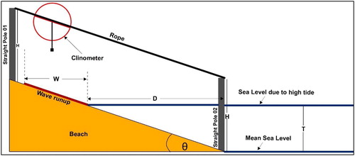
Figure 7. Flow chart showing the overall methodology adopted in this study. Note: Object size was used for spatial resolution interpretation of satellite images. GE stands for Google Earth. GPS stands for Global Positioning System. SD stands for Standard Deviation.

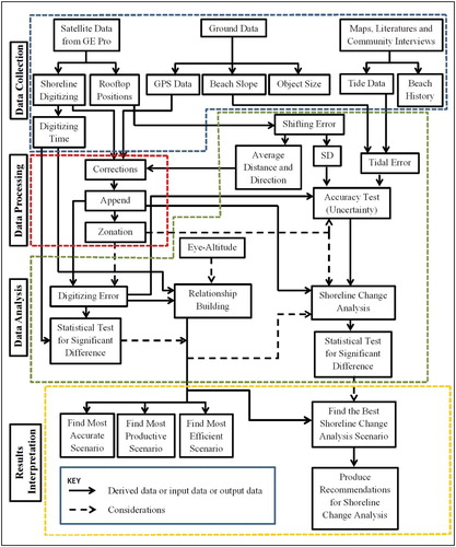
Figure 8. Derived relationships among digitizing error, time and eye-altitude (a – Relationship between eye-altitude and digitizing error, b – Linearized model of the relationship between eye-altitude and digitizing error, c – Relationship between eye-altitude and digitizing time, d – Linearized model for the relationship between eye-altitude and digitizing time, e – Relationship between normalized time and eye-altitude, f – Relationship between average digitizing speed and eye altitude).

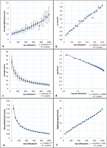
Figure 9. Relationship between shoreline length and digitizing error.

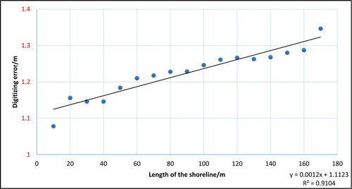
Figure 10. Derived relationships among digitizing efficincy, effectiveness and productivity (a – Relationship between digitizing error and digitizing time, b – Linearized model of the relationship between digitizing error and digitizing time, c – Relationships between percentage digitizing time and percentage digitizing error in association with eye-altitude, d – Productivity curve for shoreline digitizing from high resolution images of GE under different eye-altitudes).

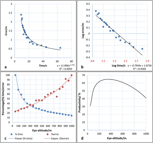
Figure 11. (a) The graph showing the distribution of digitizing error under “Append 2 scenario” (2003) along the baseline under each transect, (b) spatial distribution of digitized shorelines in 2003 under different eye-altitudes and intersected transects.

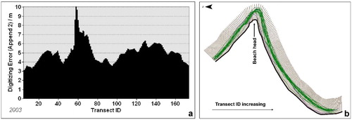
Figure 12. Digital Elevation Models of day 1 (a) and 2 (b) in northeast monsoon, day 1 (c) and day 2 (d) in southwest monsoon.

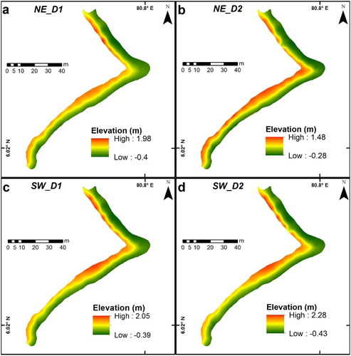
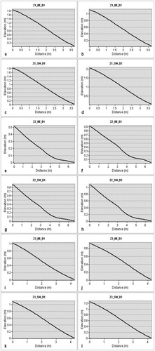
Figure 13. Selected beach profiles from the three zones over two days each of the southwest (SW) and northeast (NE) monsoon (Only middle profiles of each zone are given. Z1 – Zone 1 (a–d), Z2 – Zone 2 (e–h) Z3 – Zone 3 (i–l), D1 – Day 1, D2 – Day 2).