Extracting Coastal Water Depths from Multi-Temporal Sentinel-2 Images Using Convolutional Neural Networks

Abstract

Satellite-Derived Bathymetry (SDB) can be calculated using analytical or empirical approaches. Analytical approaches require several water properties and assumptions, which might not be known. Empirical approaches rely on the linear relationship between reflectances and in-situ depths, but the relationship may not be entirely linear due to bottom type variation, water column effect, and noise. Machine learning approaches have been used to address nonlinearity, but those treat pixels independently, while adjacent pixels are spatially correlated in depth. Convolutional Neural Networks (CNN) can detect this characteristic of the local connectivity. Therefore, this paper conducts a study of SDB using CNN and compares the accuracies between different areas and different amounts of training data, i.e., single and multi-temporal images. Furthermore, this paper discusses the accuracies of SDB when a pre-trained CNN model from one or a combination of multiple locations is applied to a new location. The results show that the accuracy of SDB using the CNN method outperforms existing works with other methods. Multi-temporal images enhance the variety in the training data and improve the CNN accuracy. SDB computation using the pre-trained model shows several limitations at particular depths or when water conditions differ.

Keywords:

• CNN
• multi-temporal images
• SDB
• Sentinel-2
• shallow water
• transfer model

Subject classification codes::

• include these here if the journal requires them

Introduction

Shallow water depth information is essential to understand the dynamics of the water bed contour characteristics. This data is essential for coastal management and research, including nautical chart production for safe navigation, coastal spatial planning, onshore buildings and ports construction planning, fishing industry, and coastal disaster mitigation. Water depth data can be obtained through a bathymetric survey. However, traditional survey methods, such as single/multi-beam echo sounding (S/MBES), have high operational costs and require a long measurement time, and the survey vessels cannot reach shallow water areas. The vessels' incapability to measure very shallow water depth, around 5 m below sea level, will cause data gaps along the shoreline area. While airborne LiDAR bathymetry could deal with this issue and produce accurate water depth data, the survey plan must consider numerous factors, including the weather for flying, air traffic control, waves, tides, ground control accessibility, turbidity, and seafloor type (Quadros 2016). Not accounting for these factors could lead to errors or even the inability to capture measurements in a particular area. Also, the operational cost is very high, so measurements using this method are still infrequent in large areas.

Since those survey methods are inefficient in measuring large water areas, especially shallow water, optical remote sensing images are a promising alternative data source for extracting water depth information. The availability of satellite imagery worldwide with different spatial and temporal resolution datasets makes it popular in various applications, including bathymetric modeling. Satellite-Derived Bathymetry (SDB) is a way to model water depth in shallow water areas using multispectral imagery. The basic principle of SDB is based on the attenuation of light in the water column. The light penetrates the water column and interacts with the water bed before the signal returns to the sensor. Once the light touches the water bed, the bottom reflectance value can be obtained from satellite images after removing other components in the atmosphere, water surface, and water column. The bottom reflectance is then used to extract water depth values.

SDB has efficiently filled data gaps with the survey method based on echo sounding. SDB is also a low-cost technique since remote sensing images are used instead of field surveys. It has few environmental impacts and risks to personnel or equipment since the model can be derived without directly accessing seawater areas. Also, water depth information can be generated relatively quickly compared to in-situ surveys. Because of this, many researchers continuously study SDB to improve the accuracy of the model and make it more efficient.

Since its initial development, many algorithms have been developed to improve the accuracy of SDB. These algorithms can be classified as analytical and empirical. The analytical methods (such as Polcyn, Brown, and Sattinger (1970), Lyzenga (1978), Favoretto et al. (2017), and Casal et al. (2020)), known as the radiative transfer model, are based on light penetration in water. It requires several optical properties of a shallow water region, such as the attenuation coefficient, backscatter coefficient, coefficient of suspended and dissolved materials, and bottom reflectance (Hengel and Spitzer 1991; Gao 2009).

In comparison, the empirical methods find the relationship between reflected radiation and in-situ depth empirically without explicitly modeling light transmission in water. The empirical methods assume that the total water reflectance is more correlated with depth than water column interaction. The linear transform method (Lyzenga 1985) and the ratio transform method (Stumpf, Holderied, and Sinclair 2003) are considered the former empirical algorithms.

Afterward, much research on SDB applied the linear and ratio transform methods, e.g., Hamylton, Hedley, and Beaman (2015), Kabiri (2017), Traganos et al. (2018), Caballero and Stumpf (2019), to different locations. Some modified the Lyzenga method (Lyzenga 1985) to improve its accuracy (Lyzenga, Malinas, and Tanis 2006; Kanno, Koibuchi, and Isobe 2011; Kanno and Tanaka 2012; Kanno et al. 2013). Kanno, Koibuchi, and Isobe (2011) stated that the improved methods had better accuracy when sufficient training data were available. There is no accuracy improvement when the data is limited. Others used different regression techniques to address the spatial heterogeneity into the model, such as Geographically Weighted Regression (Vinayaraj, Raghavan, and Masumoto 2016). However, the calibration process for this method is computationally extensive and overshooting/undershooting of the prediction becomes a major problem since the model depends on the radius used to compute the coefficients of regression. A larger radius will produce a more general prediction with fewer variations than the smaller one. Consequently, this method is limited by the number of data points or areas.

The regression techniques mentioned above only focus on the linear relationship between the ratio of water-leaving radiance in multispectral bands and depth. However, the variation of bottom types and noise in the satellite images cause the relationship to be not exactly linear. Consequently, some studies have started implementing machine learning for SDB to consider the nonlinear relationship. Machine learning is known to be able to learn a complicated relationship between input and target variables (Auret and Aldrich 2012; Sarker 2021). In the SDB case, machine learning needs to learn the relationship between water reflectance and depth to fit the model.

In the last five years, machine learning approaches such as Random Forest (Manessa et al. 2016; Sagawa et al. 2019; Tonion et al. 2020; Mateo-Pérez et al. 2021), Support Vector Machine (Misra et al. 2018; Manessa et al. 2018; Tonion et al. 2020; Mateo-Pérez et al. 2020), and Neural Networks (Liu et al. 2018; X. M. Li et al. 2020; Kaloop et al. 2022) have been used and have shown promising results. However, their spatial extent is limited to locations with in-situ coverage of depths acquired through other methods. Those methods require tuning several parameters and generating many handcrafted features to improve the algorithm. Also, they do not consider the spatial component. In SDB, spatial correlation influences the model results, assuming that pixels close together have a particular reflectance pattern linked to the depth. This characteristic of local connectivity can be captured by Convolutional Neural Networks (CNN). Several attempts to use CNN for bathymetry have been performed by Wilson et al. (2020); Mandlburger et al. (2021) in areas of groundwater (lakes). Ai et al. (2020) applied CNN to retrieve water depth in the shallow marine area from restricted remote sensing images using a single convolutional layer. However, the data may not be representative enough since it only covered two neighboring areas with clean conditions.

Most of the developed algorithms are based on the empirical method since it does not require as many physical parameters about water as the analytical method. Nevertheless, the training process still requires in-situ data to determine model coefficients that represent the relationship between reflectance and depth. That can be a major limitation of SDB since shallow water in-situ data is not available for many areas. Many studies focus on improving the model's accuracy but still require in-situ coverage. J. Li et al. (2021) provide a global shallow-water bathymetry that did not require in-situ depth in the computation but used a fixed chlorophyll-a concentration as a parameter to compute the water depth. Meanwhile, the accuracy of water depth predictions is sensitive to chlorophyll concentration, especially for areas shallower than 15 m (Kerr and Purkis 2018). On the other hand, it is now possible to use satellite-based LiDAR from ICESat-2 to get global training data (Parrish et al. 2019; Y. Li et al. 2019; Ma et al. 2020). However, another data processing algorithm is required to obtain water depth from ICESat-2 data since it does not provide shallow water depth directly.

As an alternative, this paper aims to study the transferability of a pre-trained CNN model when it is reused outside in-situ coverage, so creating SDB models without in-situ data has become possible. This paper first discusses the quality of SDB results using the CNN approach in different coastal areas before applying a pre-trained CNN model from one location to a new location.

The remainder of this paper is organized as follows. Dataset, study areas, and methods are described in Section “Materials and methods”. Section “Overview of experiments” explains the experiments. All results and discussions are provided in Section “Results and discussion”. Finally, Section “Conclusions” concludes this paper.

Materials and methods

Data

This study uses Sentinel-2 Level-2A collection images, which are atmospherically corrected. In-situ bathymetry data from LiDAR and MBES were used. They should meet the IHO Standards for Hydrographic Surveys (S-44) 5th Edition (International Hydrographic Organization 2008) for Orders special or 1, with the maximum allowable Total Vertical Uncertainty (TVU) at the 95% confidence level for a specific depth, which is given by: (1) $$\mathit{TVU}=\pm \sqrt{a^2+{\left(b\mathrm{*}d\right)}^2}$$(1) where a is the portion of the uncertainty that does not vary with depth, b is a constant, and d is the depth. The values for a and b are defined in the standard depending on the Order. For Order special, a = 0.25 m and b = 0.0075; while for Order 1a, a = 0.5 m and b = 0.013. The Order special is defined as areas where under keel clearance, the distance between the lowest point of the ship's hull or keel and the sea floor, is critical, e.g., harbors, berthing areas, and shipping channels. Meanwhile, Order 1a is for areas where under keel clearance is less critical, but features that are a concern to shipping may exist. Order 1a is limited to water shallower than 100 m. Besides these Orders, IHO specifies Order 1 b and Order 2. Order 1 b is similar to Order 1a, but the under keel clearance is not an issue here. Meanwhile, Order 2 is intended for areas deeper than 100 m.

Study area

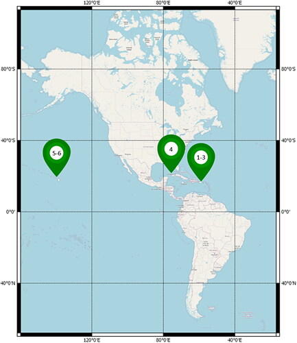
For this study, several areas (see Figure 1) were selected considering the availability of datasets that have mostly clear water conditions. The water conditions were measured visually and by looking for spectral values that differed according to the depth. Six Areas of Interest (AOIs) are scattered around the Puerto Rico's main island, southern Florida, and the Oahu island. Puerto Rico's main island is one of the locations with various coastal water characteristics. The south part of the island faces the Caribbean Sea, famous for its clear water, while the northern coast faces the North Atlantic Ocean. This situation makes the northern areas generally have bigger waves than the southern. This study used two areas in the south of the island and one in the north. The following study area is in southern Florida, which has relatively clear water that is shallower than the Puerto Rico areas. Geographically, the area is surrounded by the Bahamas and the Gulf of Mexico. These first four areas were used to analyze CNN accuracies in different cases, i.e., coastal water conditions. Meanwhile, the last two areas acted as test locations for the previous results. They are located on the Oahu island, Hawaii, between the North and South Pacific Oceans. Oahu areas generally have a high clarity level with the same depth range as Puerto Rico's coastal waters. 

Figure 1. Distribution of study areas. Source: Map data from OpenStreetMap.¹

To introduce the character of the coastal waters and in-situ depth data source, Figure 2 presents the multispectral and depth imagery visualization, while Table 1 provides the general overview of each study area. The turbidity levels are defined based on the RGB color composite image and literature studies. The waters are generally clear, except near the shore in AOI-1 and AOI-2 due to river plumes (Bejarano and Appeldoorn 2013), or beach wave resuspension strokes underwater sediments as in AOI-4 (Briceño and Boyer 2015). Both AOI-3 and AOI-5 are port areas that contain various pollutants, e.g., oil, grease, ammonia, suspended solids, pathogens, and low dissolved oxygen, as an impact of industrial operations, wastewater treatment systems, urban runoff, and sewers (Puerto Rico Environmental Quality Board (PREQB)) 2016; The Hawaii State Department of Health 2018). A full description of each study area is available in Lumban-Gaol (2021). Some areas have been studied before, such as AOI-4, AOI-5, and AOI-6. AOI-4 has been studied by Caballero and Stumpf (2019) with larger extents, covering the northern and eastern regions. The previous study used the ratio transform method to extract shallow water depths. AOI-5 has been studied by Sagawa et al. (2019) using another machine learning technique, which is Random Forest, and Landsat-8 images. AOI-6 has been studied by Lyzenga, Malinas, and Tanis (2006) using an IKONOS image and a simplified radiative transfer model, where the parameters were empirically derived based on a comparison between multispectral and measured depth values.

Figure 2. Six AOIs used in this study: AOI-1 (a), AOI-2 (b), AOI-3 (c), AOI-4 (d), AOI-5 (e) and AOI-6 (f). The left pictures show Sentinel-2 Level-2A image, and others present the in-situ depth data from LiDAR or MBES measurements.

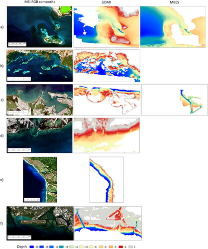
Table 1. An overview of coastal water conditions in each study area.

Area	Turbidity	Benthic habitat
AOI-1: Ponce	Low – medium	Sand, patch reefs, seagrass, algae, coral rock (Appeldoorn et al. 2016; National Oceanic and Atmospheric Administration (NOAA)) 2017)
AOI-2: Lajas	Low – medium	Sand, reefs with high coral diversity and density, seagrass, algae, rock/boulder (Bauer et al. 2012; Larsen and Webb 2009; National Oceanic and Atmospheric Administration (NOAA)) 2017)
AOI-3: San Juan	High	Sand, mud, pollutants, seagrass meadows, reefs and coral rocks outside the ports (Puerto Rico Environmental Quality Board (PREQB)) 2016)
AOI-4: Key West	Low – high	Sand, mud, seagrass, algae, live coral (National Centers for Coastal Ocean Science, n.d.)
AOI-5: Makua	Low	Sand, coral reef, rock/boulder (Hawaii State Office of Planning, n.d.; University of Hawaii 2013)
AOI-6: Honolulu	Low – medium	Sand, mud, algae, reef, pavement (University of Hawaii 2013)

Data acquisition

The Sentinel-2 Level-2A datasets are open and accessible through the Copernicus Open Access Hub.² In order to select appropriate images, this study uses the GEE³ platform to filter the Sentinel-2 Level-2A image collection based on the boundary extent of each study area and cloud pixel percentage. Additionally, the acquisition date is used to obtain multi-temporal images, i.e., one image per month throughout the year of 2019. The image collection is then sorted based on its clouds percentage, and the least cloudy image of each month is downloaded from the Copernicus database.

The availability of LiDAR and MBES data can be checked through the National Oceanic and Atmospheric Administration (NOAA) Bathymetric Data Viewer⁴. The MBES datasets are downloaded from the same source, while the LiDAR data is collected from the NOAA Data Access Viewer⁵. The LiDAR data is available as a raster or point cloud. When available, this research uses the LiDAR image products where the depths are delivered with 1 m resolution. If the LiDAR raster is not available, the point cloud is downloaded. The MBES datasets are delivered as raster with a spatial resolution of 32 m. The LiDAR and MBES images are available in AOI-1 and AOI-3, both used in these areas. For AOI-2 and AOI-3, only LiDAR raster products are available. Meanwhile, AOI-5 and AOI-6 use LiDAR point cloud instead of an image as the data source for in-situ depths. In addition, NOAA also provides tide predictions⁶ that are used for in-situ depth correction. Tidal data of each location is collected following the Sentinel-2 images' sensing date and time.

Data preprocessing

The LiDAR and MBES data have different spatial resolutions, 1 m and 32 m, respectively. Meanwhile, the spatial resolution of Sentinel-2 images is 10 m. Thus, both in-situ datasets were resampled to 10 m using nearest-neighbor interpolation with the default parameters in the QGIS⁷ software. Afterwards, both images were merged using the GDAL⁸ merge algorithm available in QGIS. It merges multiple rasters based on input arrangements where the last image overwrites the earlier ones in overlapping areas. In this case, the MBES data was set as the first image and the LiDAR as the last, so LiDAR depths were assigned as output when they overlap since these are considered more accurate. In order to synchronize disparate times between in-situ and satellite images, a tidal correction was applied to the MBES and LiDAR bathymetry data depending on the satellite image sensing time and the vertical datum. The datasets have two kinds of vertical datum: Mean Lower Low Water (MLLW) and Mean Sea Level (MSL). MLLW is the mean of the lowest tide while MSL is the average hourly height; both are recorded for 19 years. For each area, the closest tide station was selected.

A different preprocessing step was applied to AOI-5 and AOI-6 in Oahu since the LiDAR point cloud is the available data source instead of a LiDAR-derived raster. The original point cloud covers a wide range of elevation. In order to reduce the computational load when converting the data, the point cloud was filtered using LAStools⁹ to a specific range, from 4 m to −25 m, since this research focuses on up to 20 m depth. The point cloud was converted into a raster using PDAL¹⁰ with 10 m spatial resolution as output. PDAL provides several statistical methods to assign an output pixel.

In this study, the mean value of all points within the default radius, which is $\mathit{resolution}\mathrm{*}\sqrt{2}$ is used. The LiDAR point cloud still refers to the ellipsoid; consequently, the output image should be corrected to adjust the elevation to refer to the MSL datum. The product metadata provides this correction value, which is −0.601 m.

Convolutional neural networks

CNN is a promising approach in machine learning when applied to image analysis. The regular Neural Networks (NN) do not scale well to full images because the networks end up with an enormous number of parameter weights. For example, a small image with dimensions of 200x200x3 needs 120,000 weights to train in a simple NN. Therefore, the alternative approach is to use a convolution layer. Instead of having a fully connected layer where every input neuron is connected to all the hidden neurons, a neuron only is connected to a specific region of interest (usually nearby pixels) in the layer before it. By doing this, the number of connections is enormously reduced. A typical CNN architecture uses pixel values as the input layer, followed by a combination of convolutional layers, activation functions, pooling layers, and fully connected layers.

Wang et al. (2021) provide an interactive tool¹¹ to visualize how every layer in CNN works. It describes the basic CNN architecture: convolve operation, Rectified Linear Unit (ReLU) function, and regularization. A general overview of some components in CNN architecture is discussed here.

Input layer. The input layer takes an image with a particular dimension: width, height, and depth. The depth is the number of channels used to train.

Convolutional layer. The convolutional layer applies a convolutional filter that translates only a small region of every pixel and its neighborhood. The computation is based on a dot product between the filter weights and a small region connected to the input volume. The output has the same width and height as the input, and the depth refers to the number of filters used. A convolutional layer requires a set of parameters, such as the number of filters, filter extent (dimensions to convolve), stride (how many steps to skip), and padding (expanding the volume with zeroes to keep the original volume).

Activation function. The activations introduce nonlinear transformation to the network. There are several activations available, but the most common function is ReLU. It applies a function $f\left(x\right)=\max (0,x)$ to each pixel with a threshold of zero. The minimum value is zero, so negative values are converted to zero and then deactivated. Activation is also needed at the end of the network to compute the final output. For classification tasks, a sigmoid is usually used. It computes the probability of a pixel belonging to a certain class. Meanwhile, linear activation is employed to obtain continuous values in the regression task.

Fully connected layer. A fully connected layer works as a simple NN where each neuron has a connection to all neurons in the previous layer. The dimensions are $1x1xN,$ where $N$ is the number of desired outputs, e.g., the number of classes.

Model regularization. In addition to previous architectures, dropout and batch normalization may be added to perform regularization to avoid overfitting. The dropout layer randomly omits a certain proportion of neurons. Batch normalization reduces the internal covariate shift due to the randomness in the input data as well as the parameter initialization. Adding batch normalization and dropout layer into the CNN network may produce a stabler model.

CNN data preparation

This study applied raster alignment to depths and multispectral images to perfectly align both rasters. Then, sub-images with 9 × 9 window size were extracted from the data. Figure 3a provides an example of the sub-images extraction for a window size of nine and stride of three. As we can see, the amount of training data was reduced by striding the image pixels. On the other hand, Figure 3b illustrates the sub-images extraction, without striding, that is used to calculate shallow water depth on each white dot as the final output.

Figure 3. Sub-images extraction of multispectral images and depth. The pixels illustrate the surface reflectance of Sentinel-2, the white boxes are the window size of 9 × 9, and the dots indicate the water depth values. Spectral bands of each window correspond to the water depth value at the sub-image center.

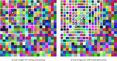
Furthermore, the LiDAR bathymetry still captures the elevation on the land, so this study filtered the elevation to include only areas up to 2 m above sea level in the sub-images. At the end of this stage, the sub-images in Figure 3a were randomly separated into training and testing sets based on the total number of sub-images, using the $\mathit{numpy}.\mathit{random}.\mathit{choice}$ function under the NumPy module. The proportion of the training, including validation, and testing sets was 80% and 20%, respectively.

CNN architecture

This study used a CNN architecture that has been studied previously in Lumban-Gaol, Ohori, and Peters (2021). The architecture differs from Ai et al. (2020) because the previous experiment indicates that training cannot converge with a single convolutional layer. The study concluded that this architecture is considered suitable for the SDB task: triple convolutional layers with 3 × 3 kernel size and batch normalization, a window size of 9 × 9, RGBNSS channel, ReLU activation at the convolution layers, linear activation at the output layer, and dropout layer. In order to optimize the model while training, the default loss function, which is the Mean Square Error (MSE), is used. The function computes the mean of squares of errors between measured and predicted depths. The squaring results in a higher error when there is a large deviation between the predicted and ground truth values. The optimizer will try to minimize that error to improve the model in each iteration. After a particular epoch, the MSE will stop improving. The training can be stopped automatically with an early stopping callback, using the MSE value to monitor the loss and a certain threshold used to stop the training. Meanwhile, this project uses a fixed 300 epochs total to monitor the training. Besides the loss function, the MSE and Mean Absolute Error (MAE) values are used as the metric to evaluate the training results by monitoring the validation accuracy on each epoch. Based on the preliminary experiments, the validation accuracy in the training process was optimal with a learning rate of 0.0001, batch size of 512, and a dropout rate of 0.3. Thus, these parameters were used as the default setting in this research.

Result assessment

The assessment of the SDB model from CNN is carried out by comparing the predicted and in-situ depth from the test data. We use a standard accuracy assessment by estimating the RMSE (Equation 2(2) $$\mathit{RMSE}=\sqrt{\frac{{\sum }_{i=1}^n{(d_{{\mathit{ref}}_i}-d_{{\mathit{pred}}_i})}^2}{n}}$$(2) ) to measure the error and the coefficient of determination R² (Equation 3(3) $$R^2=1-\frac{{\sum }_{i=1}^n{(d_{{\mathit{ref}}_i}-\mathrm{ }{d}_{{\mathit{pred}}_i})}^2}{{\sum }_{i=1}^n{(d_{{\mathit{ref}}_i}-\overline{d_{\mathit{ref}}})}^2}$$(3) ) to measure the variance of the model and the ground truth values. An additional metric, the Median Absolute Error (MedAE, Equation 4(4) $$\mathit{MedAE}=\mathit{median}\left|d_{{\mathit{ref}}_i}-d_{{\mathit{pred}}_i}\right|$$(4) ), is used to compare the existing related work. In those equations, $d_{{\mathit{ref}}_i}$ is measured depth at pixel $i,$ $d_{{\mathit{pred}}_i}$ is predicted value at the same pixel as $d_{{\mathit{ref}}_i},$ and $\overline{d_{\mathit{ref}}}$ is the mean of in-situ data. (2) $$\mathit{RMSE}=\sqrt{\frac{{\sum }_{i=1}^n{(d_{{\mathit{ref}}_i}-d_{{\mathit{pred}}_i})}^2}{n}}$$(2) (3) $$R^2=1-\frac{{\sum }_{i=1}^n{(d_{{\mathit{ref}}_i}-\mathrm{ }{d}_{{\mathit{pred}}_i})}^2}{{\sum }_{i=1}^n{(d_{{\mathit{ref}}_i}-\overline{d_{\mathit{ref}}})}^2}$$(3) (4) $$\mathit{MedAE}=\mathit{median}\left|d_{{\mathit{ref}}_i}-d_{{\mathit{pred}}_i}\right|$$(4)

Overview of experiments

SDB comparison in different locations from a single image. The CNN architecture that has been defined is applied to four study areas, which are Ponce (AOI-1), Lajas (AOI-2), San Juan (AOI-3), and Key West (AOI- 4). These areas represent three different cases. AOI-2 portrays a neighbor area of AOI-1, which is located in the same image as Ponce. AOI-3 serves as a location in the same coastal waters as AOI-1 and AOI-2, which is on Puerto Rico's main island but has a different water condition and a different image. AOI-4 represents coastal waters far from the previous areas and has different water conditions.

SDB using multi-temporal images. In general, the quality of the machine learning result depends on the quality of the input datasets used for training. The quality includes the variation of the data to obtain a generalized model. When the training data represents a given study area, it is likely to produce an accurate and reliable SDB model. This experiment aims to improve the variety of datasets using a time series of images in each location. With suitable cloud conditions, this study collects one image per month in 2019 at each location. Sub-images from each image are combined to train the model. Then, the trained model is applied to the multi-temporal images. The results are compared to the previous results from a single image on the same acquisition date.

Transfer model analysis. This experiment introduces two new datasets: Makua (AOI-5) and Honolulu (AOI-6). They are located on the Oahu island and set as test locations to test various pre-trained models in other locations. Beforehand, individual training in each area is carried out. Then, each pre-trained model from each AOI is reused in these new locations. Additionally, several combinations of training data between AOI-1 to AOI-4 are trained and tested in AOI-5 and AOI-6.

Results and discussion

SDB in different locations using a single image

The same CNN architecture was applied to several areas in the same coastal waters, i.e., AOI-1, AOI-2, and AOI-3, and in a different area, i.e., AOI-4. Table 2 presents the accuracy of each location. Note that AOI-1 to AOI-3 have the same depth range (0-20 m), while AOI-4 has a shallower range of 0-10 m. The RMSE values within the same depth range (0-10 m) in AOI-1, AOI-2, and AOI-3 are 0.91 m, 1.61 m, and 2.33 m, respectively. Additionally, Table 3 depicts the RMSE values for each increment of 5 m, indicating that the accuracy tends to decrease as the depth increases, except at 10-15 m.

Table 2. Accuracy assessment of SDB using CNN trained in AOI-1, AOI-2, AOI-3, and AOI-4.

AOI	RMSE (m)	R^2
AOI-1	1.22	0.95
AOI-2	1.63	0.93
AOI-3	3.03	0.55
AOI-4	0.73	0.94

Table 3. RMSE values per 5 m depth increment using CNN trained in AOI-1, AOI-2, AOI-3, and AOI-4.

AOI	RMSE (m)
	0-5 m	5-10 m	10-15 m	15-20 m
AOI-1	0.71	0.99	1.60	1.35
AOI-2	0.66	2.03	2.22	1.77
AOI-3	1.84	2.5	5.31	3.03
AOI-4	0.57	0.89	–	–

A more detailed assessment is provided in Figure 4, where the RMSE is calculated in increments of 1 m in depth, and in Figures 5–8. The error trend per 1 m depth range between different locations is different. Overall, AOI-3 produces a more significant error compared to other locations. Many factors presumably contribute to these errors, including the light penetration rates concerning depth and turbidity levels.

Figure 4. SDB accuracy per 1 m depth range using CNN trained in AOI-1 (orange), AOI-2 (grey), AOI-3 (yellow), and AOI-4 (blue).

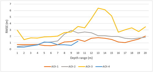
Figure 5. AOI-1 SDB model (left) and cross profiles (right). The cross-section compares the SDB model using CNN trained (blue) and in-situ depth (green).

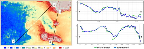
Figure 6. AOI-2 SDB model (left) and cross profiles (right). The cross-section compares the SDB model using CNN trained (blue) and in-situ depth (green).

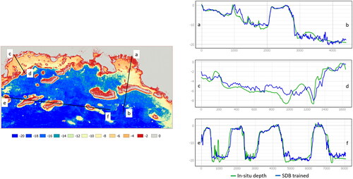
Figure 7. AOI-3 SDB model (left) and cross profiles (right). The cross-section compares the SDB model using CNN trained (blue) and in-situ depth (green).

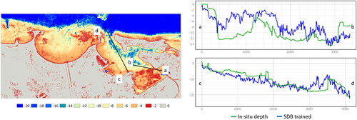
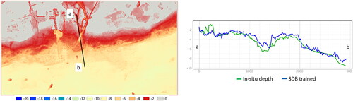
Figure 8. AOI-4 SDB model (left) and cross profiles (right). The cross-section compares the SDB model using CNN trained (blue) and in-situ depth (green).

The profile section a-b of AOI-1 (Figure 5) indicates that the SDB produces a good fit for the depths shallower than 14 m. SDB tends to fit poorer in the deeper ranges than in shallow depths. Meanwhile, the profile section c-d describes the trend over the area shallower than 14 m with land present in between. The cross-section illustrates a good fit in the SDB model, but improvements are still needed to detect the coastline area accurately. In AOI-2, Figure 6a and b shows an inaccurate SDB result compared to Figure 6c and d, which has the same depth range. It may occur when profiles a-b and c-d have different water characteristics, and the training data is not sufficient to represent areas in profile section a-b.

Figure 7 shows two cross-sections in the San Juan harbor area. The first cross profile (Figure 7a and b) compares different SDB results and in-situ depths from the east around the nearshore area, close to the estuary, to the west. It shows that the errors occur almost at all depth levels, including the very shallow area (0-5 m) where the RMSE of SDB prediction only achieves 2.06 m with an R² of 0.11. Figure 7c and d shows a similar trend where the channel is not identified well in the SDB trained. In general, the SDB results predict shallower depths than the references. Besides the noisier reflectance due to sediments or pollutants in the turbid water column, the nearshore area, especially around the estuary, may be characterized/suffer from silting due to suspended solids from the river stream. This result indicates that SDB computation encounters difficulty in more turbid waters since the reflectance values from the bottom are obscured by the particles that cause turbidity.

Figure 8 provides the visualization of the SDB results with the default setting, which indicates a good prediction considering the estuary and dredging area are visible in the SDB output. Previous research by Caballero and Stumpf (2019) used the same area but to a more considerable extent. The study used LiDAR bathymetry acquired in 2016, having the same depth range as this project, and an image from Sentinel-2 Level-1C captured on 8 February 2017. The SDB was generated based on the ratio transform method, and the accuracy was evaluated in terms of MedAE, which is 0.39 m. Using the same accuracy metric, the SDB using CNN in this research yields a better MedAE value of 0.31 m.

The light penetration rate in water for each wavelength is different. Red, green, and blue are visible, so it is possible to visually distinguish different backscatter or absorption rates based on their natural color composite. For example, water color appears blue when red and green are mostly absorbed or white when they are mostly backscattered. In AOI-3, San Juan has a large port with different and more turbid water conditions than AOI-1 and AOI-2. This condition causes different variations in reflectance, so the relationship with depth is less clear. The reflectance values in AOI-3 are generally higher and noisier than AOI-1 and AOI-2 because the particles in the water column interfere with the light spectrum in all bands and cause a more substantial backscattering effect in the water column. Meanwhile, AOI-4 has a different water condition than the study areas in Puerto Rico, where the pixels are more reflective, especially in the 0-5 m depth range, but more absorbed as well. The reflective pixels occur due to high nutrients, which correlate with more turbid waters than in other areas. The absorbed pixels, which appear darker, occur where most red, NIR, and SWIR bands are completely absorbed, so the reflectance values are almost zero. Based on the spectral reflectance plot, AOI-4 has more extensive reflectance ranges than other areas.

SDB using multi-temporal images

The number of multi-temporal images for each AOI is different due to the different availability of mostly cloud-free images in every satellite image within one year. AOI-1 and AOI-2 have complete images from January to December 2019. Meanwhile, due to cloud cover, AOI-3 and AOI-4 do not have suitable images in particular months.

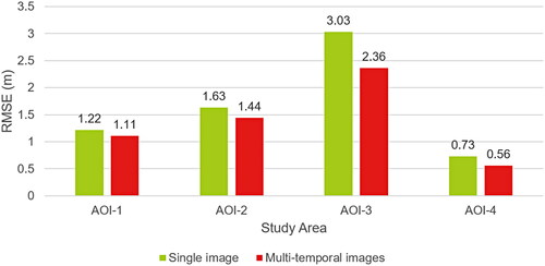
Figure 9 compares RMSE values using single and multi-temporal images in different locations. The accuracy improved when using multi-temporal images in all sites, where the RMSE at AOI-3, AOI-2, AOI-4, and AOI-1 decreased by 0.67 m, 0.19 m, 0.17 m, and 0.11 m, respectively. These results indicate that multi-temporal images enhance training data variations and benefit in areas with more noise present in the image.

Figure 9. SDB accuracy comparison between results with a single image and multi-temporal images.

The multi-temporal images indicate a seasonal variation shown by various image tones corresponding to seasonal change. For example, images of Puerto Rico's areas appear greener between October and March than in other months. Besides that, the color is also affected by the substitution of particles in the water column, where the images can appear dark, greenish, or bluish in different months. Accordingly, when all bands are mostly absorbed, the image appears darker than others. Meanwhile, when green or blue reflect more energy than other bands, the image appears greenish or bluish. Therefore, including several images in different seasons increases the variety of sample data for training, thus increasing the possibility of CNN to generalize the model.

Transfer model analysis

AOI-5 and AOI-6 represent other locations used to analyze the SDB result when reusing a pre-trained model. They are captured in different satellite footprints on the same acquisition date, 10 December 2019. The trained model's accuracy in both areas generally indicates an accurate prediction. Specifically for AOI-5, the same area has been studied by Sagawa et al. (2019) using another machine learning approach, i.e., Random Forest, and Landsat-8 surface reflectance product, which is atmospherically corrected. That study used 26 multi-temporal images from 2013 to 2018, and 9,974 data pixels were used for training. In terms of RMSE, the maximum accuracy was 1.24 m with an R² of 0.93. Compared to the same area, with less training data (5,851), this study yields a better RMSE of 0.79 m with an R2 of 0.98. Table 4 provides RMSE and R² values in AOI-5 and AOI-6 using various CNN models calculated in Section “SDB using multi-temporal images”.

Table 4. SDB accuracy in AOI-5 and AOI-6 using the trained model, pre-trained model of different study areas, and bathymetry model from Allen Coral Atlas.

CNN model	AOI-5		AOI-6
	RMSE (m)	R^2	RMSE (m)	R^2
Trained	0.79	0.98	1.34	0.94
Pre-trained on AOI-1	2.61	0.79	3.16	0.73
Pre-trained on AOI-2	2.92	0.69	2.98	0.71
Pre-trained on AOI-3	7.42	0.13	6.42	0.16
Pre-trained on AOI-4	6.84	−7.56	5.56	−4.72
Allen Coral Atlas	3.19	0.73	2.99	0.79
Sagawa et al. (2019)	1.24	0.93	–	–
Lyzenga, Malinas, and Tanis (2006)	–	–	3.01	–

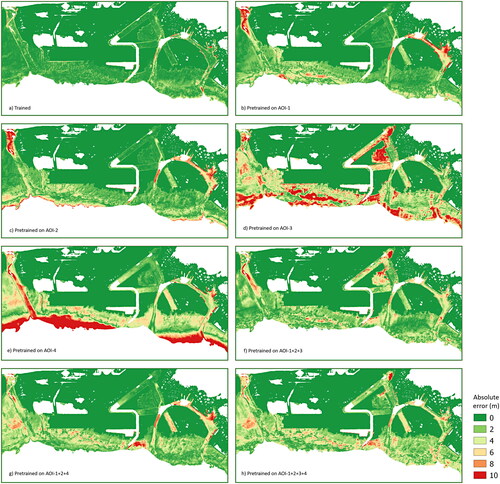
Figures 10–15 demonstrate prediction vs ground truth plots, SDB models, and absolute error maps in AOI-5 and AOI-6, respectively. SDB results in AOI-5 and AOI-6 using the pre-trained models indicate discrepancy with the in-situ depths or SDB trained. When the pre-trained model of AOI-1 is used to build the SDB model in AOI-5, the prediction results tend to fit the references until 15 m depth (see Figure 10b). However, in areas deeper than that, the calculated depths include significant errors where the values are predicted to be shallower or deeper than the measured depths. In general, the SDB models become deeper when using other pre-trained models, except when using the pre-trained model at AOI-4, where the result shows a completely different trend as presented in Figure 10e with absolute error illustrated in Figure 12e. It shows that the pre-trained model from AOI-4 cannot predict areas deeper than 10 m. Moreover, errors in Figure 11c mostly appear in deeper areas, with a sandy bottom, than in shallow waters, with coral reefs and hardbottom, especially from the northern to the middle (see Figure 12b).

Figure 10. Prediction vs reference depth plots in AOI-5 using different CNN models: trained (a); pre-trained on AOI-1 (b); pre-trained on AOI-2 (c); pre-trained on AOI-3 (d); pre-trained on AOI-4 (e); pre-trained on the combined AOI-1, AOI-2, and AOI-3 (f); pre-trained on the combined AOI-1, AOI-2, and AOI-4 (g); pre-trained on the combined AOI-1, AOI-2, AOI-3, and AOI-4 (h).

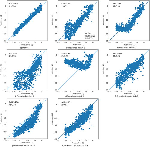
Figure 11. LiDAR bathymetric depths (a) and SDB results in AOI-5 using different CNN models: trained (b); pre-trained on AOI-1 (c); pre-trained on AOI-2 (d); pre-trained on AOI-3 (e); pre-trained on AOI-4 (f); pre-trained on the combined AOI-1, AOI-2, and AOI-3 (g); pre-trained on the combined AOI-1, AOI-2, and AOI-4 (h); pre-trained on the combined AOI-1, AOI-2, AOI-3, and AOI-4 (i).

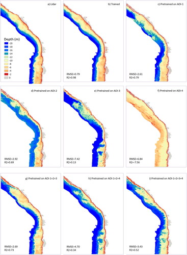
Figure 12. Absolute error of SDB per pixel when using different CNN models: trained (a), pre-trained on AOI-1 (b); pre-trained on AOI-2 (c); pre-trained on AOI-3 (d); pre-trained on AOI-4 (e); pre-trained on the combined AOI-1, AOI-2, and AOI-3 (f); pre-trained on the combined AOI-1, AOI-2, and AOI-4 (g); pre-trained on the combined AOI-1, AOI-2, AOI-3, and AOI-4 (h).

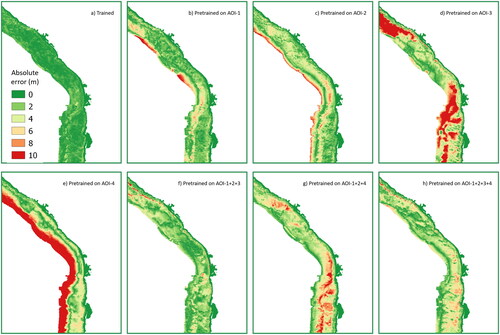
Figure 13. Prediction vs reference depth plots in AOI-6 using different CNN models: trained (a); pre-trained on AOI-1 (b); pre-trained on AOI-2 (c); pre-trained on AOI-3 (d); pre-trained on AOI-4 (e); pre-trained on the combined AOI-1, AOI-2, and AOI-3 (f); pre-trained on the combined AOI-1, AOI-2, and AOI-4 (g); pre-trained on the combined AOI-1, AOI-2, AOI-3, and AOI-4 (h).

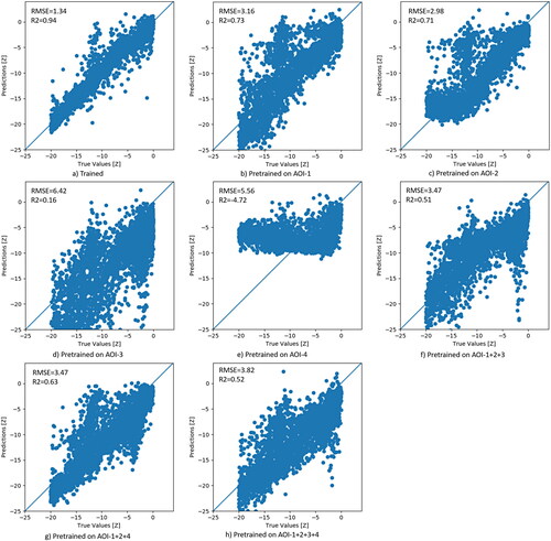
Figure 14. LiDAR bathymetric depths (a) and SDB results in AOI-6 using different CNN models: trained (b); pre-trained on AOI-1 (c); pre-trained on AOI-2 (d); pre-trained on AOI-3 (e); pre-trained on AOI-4 (f); pre-trained on the combined AOI-1, AOI-2, and AOI-4 (g); pre-trained on the combined AOI-1, AOI-2, and AOI-4 (h); pre-trained on the combined AOI-1, AOI-2, AOI-3, and AOI-4 (i).

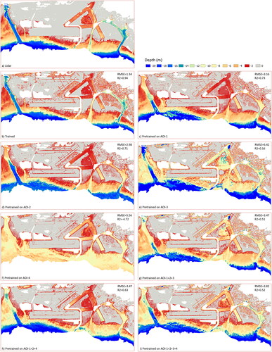
Figure 15. Absolute error of SDB per pixel when using different CNN models: trained (a), pre-trained on AOI-1 (b); pre-trained on AOI-2 (c); pre-trained on AOI-3 (d); pre-trained on AOI-4 (e); pre-trained on the combined AOI-1, AOI-2, and AOI-3 (f); pre-trained on the combined AOI-1, AOI-2, and AOI-4 (g); pre-trained on the combined AOI-1, AOI-2, AOI-3, and AOI-4 (h).

For another comparison, Figures 13 and 14 portray different SDB results in AOI-6. As mentioned in Section “Study area”, Honolulu is another port area, so the disturbance of reflectance due to water turbidity is more substantial than in Makua. More dredged bottoms also appear in this area. Although the result is not as accurate as AOI-5 within the same depth range, the RMSE is better than the San Juan port. Figure 13a points out that several depth values are predicted to be too shallow, and Figure 14a shows that it occurs in the western channel, which is a dredge zone. The other dredged areas also appear shallower than the measured depth. This circumstance is similar to the San Juan area. However, even though they share the same characteristics around the harbor, the pre-trained model from San Juan is incompatible with the data for Honolulu, as shown in Figures 13d, 14e, and 15d.

Additionally, the pre-trained model of AOI-4 is also unable to calculate the SDB in AOI-6. Therefore, the pre-trained model of AOI-4 is incompatible for Oahu regions as the shallow water was calculated to have deeper values and vice versa. The fact that the pre-trained model of AOI-4 resulted in shallower predictions at the 10-20 depth range is related to the fact that the AOI-4 training data only covers 0-10 m depths. Besides different reflectance characteristics, in the case of AOI-4, the pre-trained model does not represent the entire depth range.

Another study using the radiative transfer model in AOI-6 was performed by Lyzenga, Malinas, and Tanis (2006) using an IKONOS multispectral image. With a combination of empirical and analytical methods, the study yielded an RMSE of 3.01 m. In this study, the accuracy of the SDB using the trained model is 1.34 m, while the optimum accuracy when reusing the pre-trained model from another location is 2.98 m. The simplified radiative model delivers a similar accuracy to the computed SDB using the pre-trained CNN model, but it still requires in-situ depths within the study area to derive the physical parameters empirically. In the case of the transfer model of CNN, no measured depth is needed anymore so that the SDB can be derived directly.

Additionally, we compare the transferability results in AOI-5 and AOI-6 with the global shallow-water bathymetry produced by J. Li et al. (2021). Using the same extent as our study area, we downloaded the bathymetry data from the Allen Coral Atlas website¹² and computed the RMSE using the same ground truth data and depth range. The accuracies are 3.19 m and 2.99 m for AOI-5 and AOI-6, respectively (see Table 4). The results show that our method is comparable to the Allen Coral Atlas product, even better by roughly 0.4 m in AOI-5.

Nevertheless, the SDB generated using the pre-trained model has a wide range of accuracies, which becomes a drawback since choosing which pre-trained model to use is not easy. Extra knowledge about the coastal water characteristics, such as chlorophyll concentration and turbidity, may help select an appropriate pre-trained model considering similar water conditions are more suitable for implementing the transfer model than a different one. Also, it is better to keep verifying the result with the measured depth. Our experiments show that the trained model SDB results in better accuracy than the pre-trained model in the 1.64 m − 2.13 m range for the pre-trained model of AOI-1 and AOI-2 and the 4.22 m − 6.63 m range for AOI-3 and AOI-4.

A similar experiment of the transfer model was performed in the central part of the South China Sea, on a small island of 0.3 km² named Robert Island, where the water depth was computed using a pre-trained model from its neighboring island named North Island (Ai et al. 2020). In terms of Mean Absolute Error (MAE), the accuracy of the trained model in the North Island using a ZY3 image is around 0.668 m to 0.785 m in different depth ranges. The accuracy reached 0.95 m on the Robert Island using the pre-trained model. However, we cannot measure the relative performance of the transfer model with the trained model since the study did not train the Robert Island area.

Furthermore, this project combines training data from several locations to produce a more generalized CNN model. The assumption is that the combined training data will enrich the variation of reflectances concerning different water column compositions and bottom types in different depth ranges. Nevertheless, SDB results using several training datasets show inaccurate outputs compared to the single data from AOI-1 or AOI-2. This issue might be caused by unbalanced training because a particular location provides more information than others. In an attempt to solve this problem, this study tries to balance the data in a combination of AOI-1, AOI-2, AOI-3, and AOI-4 by undersampling and oversampling, taking the number of training data per location into consideration. For the undersampling case, the proportion of training data in AOI-2 and AOI-4 was reduced by 50%, considering the number of training data in AOI-2 is double that of others, and AOI-4 only covers the 0-10 m depth range. However, the accuracy is lower than the original combination without undersampling, which is 4.70 m and 0.34 for the RMSE and the R2, respectively. It occurs possibly because the undersampling method removes some details in the training data. On the other hand, the oversampling case increases the number of training data in AOI-1 by copying the existing data. The oversampling method obtains inaccurate results with RMSE and R2 of 7.4 m and 0.26, respectively.

These results pinpoint that SDB calculation using a pre-trained model is likely affected by water characteristics. In this case, AOI-5 and AOI-6 water characteristics are more alike with AOI-1 or AOI-2 than AOI-3 or AOI-4. The combination of pre-trained models shows the difficulty of CNN to fit the training data from different locations to a new location, even if the new location has similar characteristics to one of them. To study the transfer model comprehensively, a rigorous technique to create balanced training data should be considered. Several water characteristics, such as water color, chlorophyll concentration, and turbidity, should be considered while combining training data from different locations, even though they have the same bottom types.

Conclusions

The results show that SDB accuracies depend on the local characteristics of the coastal water. In this case, turbid water has a more significant error than clean water. Thus, SDB is not suitable to be used in the turbid area. The improved accuracy of SDB in different locations occurs when using multi-temporal images instead of a single image only. Therefore, adding temporal variation in the training data helps generalize the training model and improve the accuracy of SDB. Compared to existing works, the accuracy of SDB using CNN outperform other methods, such as ratio transform, radiative transfer model, and Random Forest.

Implementing the pre-trained models of different study areas, or their combination, to the new areas yields a wide range of accuracy. Some pre-trained models are more suitable for reusing than others, but the output is reliable only at particular depth ranges. Meanwhile, other pre-trained models are not suitable for reusing due to a lack of data at particular depths or reflectances that are too noisy. The pre-trained model of turbid waters at the harbor area tends to apply to local areas only, meaning that the pre-trained model is unsuitable for reuse even if the new area is also a harbor because the turbidity rate may differ, so the level of noise in the reflectance is not the same.

Combining several training datasets from different study areas also yields a lower accuracy. It can be argued that the combination did not represent balanced training data, resulting in an unreliable trained model. Hence, supplementary information concerning the bottom types and water column properties helps preserve the variety of data. Since the accuracies diverge, it is hard to predict which pre-trained model is compatible with which data. Therefore, besides having the supplementary data, verifying the SDB model using measured depths considering the risk when computing the SDB using a pre-trained model is recommended.

Disclosure statement

No potential conflict of interest was reported by the authors.

Data availability statement

A complete set of codes, including sample data, is provided in the Github repository at https://github.com/yustisiardhitasari/sdbcnn. The data that support the findings of this study are openly available in the Copernicus Open Access Hub at https://scihub.copernicus.eu/, the National Oceanic and Atmospheric Administration (NOAA) Bathymetric Data Viewer at https://www.ncei.noaa.gov/maps/bathymetry/ and the NOAA Data Access Viewer at https://coast.noaa.gov/dataviewer/. Map data copyrighted OpenStreetMap contributors and available from https://www.openstreetmap.org

Additional information

Funding

This work was supported by the Indonesian Endowment Fund for Education (LPDP) and the European Research Council (ERC) under the European Union's Horizon 2020 research and innovation programme (grant agreement No 677312 UMnD).

Notes

1 https://www.openstreetmap.org/copyright

2 https://scihub.copernicus.eu/

3 https://earthengine.google.com/

4 https://www.ncei.noaa.gov/maps/bathymetry/

5 https://coast.noaa.gov/dataviewer/

6 https://tidesandcurrents.noaa.gov/

7 https://www.qgis.org

8 https://gdal.org

9 https://rapidlasso.com/lastools/

10 https://pdal.io/

11 https://poloclub.github.io/cnn-explainer/

12 https://allencoralatlas.org/

References

- Ai, B., Z. Wen, Z. Wang, R. Wang, D. Su, C. Li, and F. Yang. 2020. Convolutional neural network to retrieve water depth in marine shallow water area from remote sensing images. IEEE Journal of Selected Topics in Applied Earth Observations and Remote Sensing 13:2888–98.
- Appeldoorn, R., D. Ballantine, I. Bejarano, M. Carlo, M. Nemeth, E. Otero, F. Pagan, H. Ruiz, N. Schizas, C. Sherman, et al. 2016. Mesophotic coral ecosystems under anthropogenic stress: A case study at Ponce, Puerto Rico. Coral Reefs 35 (1):63–75.
- Auret, L., and C. Aldrich. 2012. Interpretation of nonlinear relationships between process variables by use of random forests. Minerals Engineering 35:27–42.
- Bauer, L. J., E. Kimberly, K. K. Roberson, M. S. Kendall, S. Tormey, and T. A. Battista. 2012. Shallow-water benthic habitats of southwest Puerto Rico. NOAA Technical Memorandum NOAA NOS NCCOS 155:37. http://aquaticcommons.org/14709/1/SWPR_mapping_final_report_tagged.pdf.
- Bejarano, I., and R. S. Appeldoorn. 2013. Seawater turbidity and fish communities on coral reefs of Puerto Rico. Marine Ecology Progress Series 474:217–26.
- Briceño, H. O., and J. N. Boyer. 2015. 2014 Annual Report of the Water Quality Monitoring Project for the Water Quality Protection Program of the Florida Keys National Marine Sanctuary. Miami, Florida: Florida International University.
- Caballero, I., and R. P. Stumpf. 2019. Retrieval of Nearshore Bathymetry from Sentinel-2A and 2B Satellites in South Florida Coastal Waters. Estuarine, Coastal and Shelf Science 226:106277.
- Casal, G., P. Harris, X. Monteys, J. Hedley, C. Cahalane, and T. McCarthy. 2020. “ Understanding Satellite-Derived Bathymetry Using Sentinel 2 Imagery and Spatial Prediction Models. GIScience and Remote Sensing 57 (3): 271–286. https://doi.org/10.1080/15481603.2019.1685198.
- Favoretto, F., Y. Morel, A. Waddington, J. Lopez-Calderon, M. Cadena-Roa, and A. Blanco-Jarvio. 2017. Testing of the 4SM method in the Gulf of California suggests field data are not needed to derive satellite bathymetry. Sensors 17 (10):2248.
- Gao, J. 2009. Bathymetric mapping by means of remote sensing: Methods, accuracy and limitations. Progress in Physical Geography: Earth and Environment 33 (1):103–16.
- Hamylton, S. M., J. D. Hedley, and R. J. Beaman. 2015. Derivation of high-resolution bathymetry from multispectral satellite imagery: A comparison of empirical and optimisation methods through geographical error analysis. Remote Sensing 7 (12):16257–73.
- Hawaii State Office of Planning. n.d. “Hawaii Statewide GIS.” https://geoportal.hawaii.gov/datasets/.
- International Hydrographic Organization. 2008. “IHO Standards for Hydrographic Surveys (S-44) 5th Edition.” Monaco: International Hydrographic Bureau. https://iho.int/.
- Kabiri, K. 2017. Discovering optimum method to extract depth information for nearshore coastal waters from sentinel-2A imagery-case study: Nayband Bay, Iran. International Archives of the Photogrammetry. The International Archives of the Photogrammetry, Remote Sensing and Spatial Information Sciences XLII-4/W4 (4W4):105–10.
- Kaloop, M. R., M. El-Diasty, J. W. Hu, and F. Zarzoura. 2022. Hybrid artificial neural networks for modeling shallow-water bathymetry via satellite imagery. IEEE Transactions on Geoscience and Remote Sensing 60:1–11.
- Kanno, A., and Y. Tanaka. 2012. Modified Lyzenga’s method for estimating generalized coefficients of satellite-based predictor of shallow water depth. IEEE Geoscience and Remote Sensing Letters 9 (4):715–9.
- Kanno, A., Y. Koibuchi, and M. Isobe. 2011. Shallow water bathymetry from multispectral satellite images: Extensions of Lyzenga’s method for improving accuracy. Coastal Engineering Journal 53 (4):431–50.
- Kanno, A., Y. Tanaka, A. Kurosawa, and M. Sekine. 2013. Generalized Lyzenga’s predictor of shallow water depth for multispectral satellite imagery. Marine Geodesy 36 (4):365–76.
- Kerr, J. M., and S. Purkis. 2018. An algorithm for optically-deriving water depth from multispectral imagery in coral reef landscapes in the absence of ground-truth data. Remote Sensing of Environment 210 (210):307–24.
- Larsen, M. C., and R. M. Webb. 2009. Potential effects of runoff, fluvial sediment, and nutrient discharges on the coral reefs of Puerto Rico. Journal of Coastal Research 251:189–208.
- Li, J., D. E. Knapp, M. Lyons, C. Roelfsema, S. Phinn, S. R. Schill, and G. P. Asner. 2021. Automated global shallowwater bathymetry mapping using google earth engine. Remote Sensing 13 (8):1469.
- Li, X. M., Y. Ma, Z. H. Leng, J. Zhang, and X. X. Lu. 2020. High-accuracy remote sensing water depth retrieval for coral islands and reefs based on LSTM neural network. Journal of Coastal Research 102 (sp1): 21–32. https://doi.org/10.2112/SI102-003.1
- Li, Y., H. Gao, M. F. Jasinski, S. Zhang, and J. D. Stoll. 2019. Deriving high-resolution reservoir bathymetry from ICESat-2 prototype photon-counting lidar and landsat imagery. IEEE Transactions on Geoscience and Remote Sensing 57 (10):7883–93.
- Liu, S., L. Wang, H. Liu, H. Su, X. Li, and W. Zheng. 2018. Deriving bathymetry from optical images with a localized neural network algorithm. IEEE Transactions on Geoscience and Remote Sensing 56 (9):5334–42.
- Lumban-Gaol, Y. A. 2021. “Convolutional Neural Networks for Satellite-Derived Bathymetry.” Delft University of Technology. http://resolver.tudelft.nl/uuid:662ac71f-6373-4128-8eeb-163b8e727b72.
- Lumban-Gaol, Y. A., K. A. Ohori, and R. Y. Peters. 2021. Satellite-derived bathymetry using convolutional neural networks and multispectral sentinel-2 images. The International Archives of the Photogrammetry, Remote Sensing and Spatial Information Sciences XLIII-B3-2021:201–7.
- Lyzenga, D. R. 1978. Passive remote sensing techniques for mapping water depth and bottom features. Applied Optics 17 (3):379–83.
- Lyzenga, D. R. 1985. Shallow-water bathymetry using combined lidar and passive multispectral scanner data. International Journal of Remote Sensing 6 (1):115–25.
- Lyzenga, D. R., N. P. Malinas, and F. J. Tanis. 2006. Multispectral bathymetry using a simple physically based algorithm. IEEE Transactions on Geoscience and Remote Sensing 44 (8):2251–9.
- Ma, Y., N. Xu, Z. Liu, B. Yang, F. Yang, X. H. Wang, and S. Li. 2020. Satellite-derived bathymetry using the ICESat-2 lidar and sentinel-2 imagery datasets. Remote Sensing of Environment 250:112047.
- Mandlburger, G., M. Kölle, H. Nübel, and U. Soergel. 2021. BathyNet: A deep neural network for water depth mapping from multispectral aerial images. PFG – Journal of Photogrammetry, Remote Sensing and Geoinformation Science 89 (2):71–89.
- Manessa, M. D. M., A. Kanno, M. Sekine, M. Haidar, K. Yamamoto, T. Imai, and T. Higuchi. 2016. Satellite-derived bathymetry using random forest algorithm and worldview-2 imagery. Geoplanning: Journal of Geomatics and Planning 3 (2):117.
- Manessa, M. D. M., M. Haidar, M. Hartuti, and D. K. Kresnawati. 2018. Determination of the best methodology for bathymetry mapping using spot 6 imagery: A study of 12 empirical algorithms. International Journal of Remote Sensing and Earth Sciences (IJReSES) 14 (2):127.
- Mateo-Pérez, V., M. Corral-Bobadilla, F. Ortega-Fernández, and E. P. Vergara-González. 2020. Port bathymetry mapping using support vector machine technique and sentinel-2 satellite imagery. Remote Sensing 12 (13):2069.
- Mateo-Pérez, V., M. Corral-Bobadilla, F. Ortega-Fernández, and V. Rodríguez-Montequín. 2021. Determination of water depth in ports using satellite data based on machine learning algorithms. Energies 14 (9):2486.
- Misra, A., Z. Vojinovic, B. Ramakrishnan, A. Luijendijk, and R. Ranasinghe. 2018. Shallow water bathymetry mapping using support vector machine (SVM) technique and multispectral imagery. International Journal of Remote Sensing 39 (13):4431–50.
- National Centers for Coastal Ocean Science. n.d. “Florida Keys National Marine Sanctuary Digital Atlas.” https://www.arcgis.com/apps/webappviewer/index.html?id=03daf1d686c84ece8172ed394e287c78.
- National Oceanic and Atmospheric Administration (NOAA). 2017. “Benthic Habitat Mapping in Puerto Rico and the U.S. Virgin Islands for a Baseline Inventory.” 2017. https://coastalscience.noaa.gov/project/benthic-habitat-mapping-puerto-rico-virgin-islands/.
- Parrish, C. E., L. A. Magruder, A. L. Neuenschwander, N. Forfinski-Sarkozi, M. Alonzo, and M. Jasinski. 2019. Validation of ICESat-2 ATLAS Bathymetry and Analysis of ATLAS’s Bathymetric Mapping Performance. Remote Sensing 11 (14):1634.
- Polcyn, F. C., W. Brown, and I. Sattinger. 1970. “The Measurement of Water Depth by Remote Sensing Techniques.” Ann Arbor, Michigan: The University of Michigan.
- Puerto Rico Environmental Quality Board (PREQB). 2016. “Puerto Rico 305(b)/303(d) Integrated Report,” no. November: 243. http://www2.pr.gov/agencias/jca/Documents/AreasProgramáticas/AreaCalidaddeAgua/PlanesyProyectosEpeciales/303-305/2014/PuertoRico2014305b303dIntegratedReportAugust2014.pdf.
- Quadros, N. D. 2016. “Technology in Focus: Bathymetric Lidar.” GIM International, November 2016. https://www.gim-international.com/content/article/technology-in-focus-bathymetric-lidar-2.
- Sagawa, T., Y. Yamashita, T. Okumura, and T. Yamanokuchi. 2019. Satellite derived bathymetry using machine learning and multi-temporal satellite images. Remote Sensing 11 (10):1155.
- Sarker, I. H. 2021. Machine learning: Algorithms, real-world applications and research directions. SN Computer Science 2 (160). https://doi.org/10.1007/s42979-021-00592-x.
- Stumpf, R. P., K. Holderied, and M. Sinclair. 2003. Determination of water depth with high-resolution satellite imagery over variable bottom types. Limnology and Oceanography 48 (1part2):547–56.
- Hengel, Van, and D. Spitzer. 1991. “Multi-Temporal Water Depth Mapping by Means of Landsat TM.” International Journal of Remote Sensing 12 (4). https://doi.org/10.1080/01431169108929687.
- The Hawaii State Department of Health. 2018. 2018 State of Hawaii Water Quality Monitoring and Assessment Report, Honolulu, Hawaii.
- Tonion, F., F. Pirotti, G. Faina, and D. Paltrinieri. 2020. A machine learning approach to multispectral satellite derived bathymetry. ISPRS Annals of the Photogrammetry, Remote Sensing and Spatial Information Sciences V-3-2020 (3):565–70.
- Traganos, D., D. Poursanidis, B. Aggarwal, N. Chrysoulakis, and P. Reinartz. 2018. Estimating satellite-derived bathymetry (SDB) with the google earth engine and sentinel-2. Remote Sensing 10 (6):859–18.
- University of Hawaii. 2013. “Ohau Coastal Geology.” 2013. http://www.soest.hawaii.edu/coasts/publications/hawaiiCoastline/oahu.html.
- Vinayaraj, P., V. Raghavan, and S. Masumoto. 2016. Satellite-derived bathymetry using adaptive geographically weighted regression model. Marine Geodesy 39 (6):458–78.
- Wang, Z. J., R. Turko, O. Shaikh, H. Park, N. Das, F. Hohman, M. Kahng, and D. H. Polo Chau. 2021. CNN Explainer: Learning convolutional neural networks with interactive visualization. IEEE Transactions on Visualization and Computer Graphics 27 (2):1396–406.
- Wilson, B., N. C. Kurian, A. Singh, and A. Sethi. 2020. Satellite-derived bathymetry using deep convolutional neural network. In International Geoscience and Remote Sensing Symposium (IGARSS).