Building blocks of a heterodox business cycle theory

Abstract

A key characteristic of heterodox theories of the business cycle is their focus on endogenous business cycle mechanisms. This paper provides an overview and comparison of four models in heterodox business cycle theory: multiplier-accelerator models, Goodwin models, Minskyan debt-cycle models, and momentum trader models. A representative model from each theory is formulated as a two-dimensional predator-prey system in continuous time, which allows us to identify the different stabilizing and destabilizing mechanisms. We argue that the theories are substantially competing, as they posit different mechanisms that explain cycles, but we also argue that these mechanisms are not mutually exclusive. We suggest that heterodox economists work toward a synthesis.

Keywords:

• Business cycles
• Endogenous cycles
• Crises

JEL Classifications:

• B41
• B50
• E32

1. Introduction

Business cycles are back on the research agenda. After a period of abeyance, a number of papers have been published in highly respected journals arguing for a return to the study of cyclical dynamics. Beaudry, Galizia, and Portier (2020) advocates the return of ‘the cycle’ in business cycle analysis. Aikman, Haldane, and Nelson (2015) and Borio (2014) have identified regular cyclical fluctuations in financial variables and have proved very influential. This resurgence of interest in endogenous business cycles is in tension with a mainstream macroeconomics based on the (essentially neoclassical) hypothesis that markets are self-regulating, which regards business cycles as the economy’s response to exogenous shocks in the presence of frictions.¹ Heterodox economics, in contrast, has a strong tradition in theorizing business cycles as systematic outcomes of market economies. Specifically, business cycles are understood as endogenous cycles rooted in the structure of the economy, rather than a dynamic reaction to exogenous shocks. To a greater degree than mainstream economics, however, heterodox business cycle theory is strongly segmented. Kaldorian, Goodwinian, Minskyan and momentum trader traditions coexist without much direct interaction.

At the heart of early Keynesian business cycle theory was the volatility of investment expenditures. This gave rise to multiplier-accelerator models (Samuelson 1939) and to the Kaldor trade cycle model (Kaldor 1940). These models focus on the destabilizing role of investment expenditure, modeled using an accelerator function. Cyclical dynamics then result from the interaction of the accelerator with a conventional Keynesian consumption function. These models were popular in the postwar era, but have attracted much less attention recently. On the Marxian side, the seminal Goodwin (1967) model placed class struggle at the center of business cycles. In the course of an economic boom, the industrial reserve army gets depleted, which results in wage pressure and ultimately in a profit squeeze that leads to declines in investment and growth. Minskyan debt cycle models were developed later but, in a notable difference to the previous heterodox streams, there is no canonical Minskyan model. What all Minskyan models share, however, is an emphasis on financial factors. Thus debt, interest rates and asset prices play key roles in expansions as well as recessions. Momentum trader models build on Keynesian and non-Keynesian analyses of financial markets, and argue that investors are not fully rational, and that behavioral heterogeneity is a key factor in cyclical dynamics. Momentum trader models, for example, demonstrate that the interaction of fundamentalist and extrapolative price expectation rules can result in endogenous financial cycles.

The aim of this paper is to take stock of heterodox business cycle theories. Its main contribution is to compare and contrast their similarities using a consistent, transparent analytical framework. We argue that all of these business cycle theories rely on the interaction of a stabilizing and a destabilizing force. In the multiplier-accelerator, Goodwin, Minskyan debt-cycle and momentum trader theories, different sectors are involved in generating cyclical dynamics. In the multiplier-accelerator model the interaction is within the goods markets, and business cycles result from an interplay of the demand effects of investment and its reaction to excess capacity. In the Goodwin model the cycle results from goods market and labor market interactions. Growth leads to tighter labor markets, which leads to a shift in income distribution. In Minskyan debt-cycle models the cycle results from goods market and financial market interactions. Debt increases relative to income in booms, which increases financial fragility. In the momentum trader models both the stabilizing and destabilizing forces are located in financial markets, crystallized in different investment strategies and corresponding ways of forming expectations about future asset prices. Thus, the four theories emphasize different markets (or sectors) that are involved in generating the cyclical dynamics.

We argue that all four business cycle theories are theoretically consistent and give rise to endogenous cycles, but that progress in heterodox business cycle theory has been hampered by a lack of communication. As demonstrated in Stockhammer and Michell (2017), looking at business cycle theories in isolation may give misleading results. We argue for the integration of these models and that they share a common framework of animal spirits and adaptive learning. While not always made explicit, this approach to economic behavior underlies the momentum trader theory as well as those theories that posit destabilizing investment dynamics. Indeed, the multiplier-accelerator models, Goodwin models and Minskyan models can all be thought of as sharing a destabilizing goods market, but present stabilizing forces located in different sectors of the economy (the goods market, labor market and financial markets, respectively). Thus, there are logical grounds for a synthesis. We hope that this paper will encourage increased cross-fertilization between the different streams of heterodox theory.

In this paper, we use a broad, inclusive notion of heterodox business cycle theories to subsume any approach that is critical of the mainstream models that assume substantive rationality (Simon 1976). In fact, the term ‘mainstream’ changes over time, and the theories we discuss have different relationships with it (or, alternatively, different degrees of heterodoxy). The Goodwin and Minskyan models that we consider are clearly situated outside the mainstream. The multiplier-accelerator model was once mainstream, or at least an acceptable approach within mainstream economics, but is currently almost exclusively used by heterodox economists (or mathematical economists primarily interested in phenomena like chaos and complexity). The momentum trader approach sits closer to the mainstream, as it pays closer attention to what one might want to call microfoundations. However, these are arguably heterodox foundations that emphasize heterogeneity and bounded (or procedural) rationality. Our aim is to support a conversation between the various streams of heterodoxy, and thus we cast our theoretical net as wide as possible.

Our paper complements a number of existing surveys of heterodox business cycle theories. Skott (2012) provides a concise introduction to heterodox business cycles in the Elgar Companion to Post Keynesian Economics, and Bernard et al. (2014) review theories of long waves that touch on the business cycle theories we discuss. More recently, Barrales-Ruiz et al. (2022) survey theories of distributive cycles, and discuss the existing empirical evidence. Compared with these papers, our main contribution is to set the major heterodox business cycle theories in a consistent analytical framework, to allow the various stabilizing and destabilizing mechanisms to be compared in a straightforward fashion. Perhaps closest in spirit to our approach is Arnold (2002), who derives univariate autoregressive models for various mainstream business cycle theories, including monetarist, real business cycle, and New Keynesian theories, as well as the classic multiplier-accelerator model.

The paper is structured as follows. Section 2 presents a benchmark framework for the analysis of endogenous business cycles in the context of two-dimensional predator-prey models. Section 3, 4, 5 and 6 discuss the four families of heterodox business cycle theory already mentioned. For each of these we present some historical background, analyze a baseline model, and discuss models that extend beyond the baseline. Section 7 compares the theories to each other, and discusses the possibility of a synthesis.

2. A minimalist framework for analyzing business cycle theories

Business cycle models are concerned with the regular succession of periods of higher and lower growth in capitalist economies.² Formal business cycle models focus on bounded fluctuations around isolated equilibria. In this paper we cast all of the business cycle models surveyed as deterministic two-dimensional systems of ordinary differential equations, which allows the key elements of the models to be illustrated in the simplest possible manner. The general form of the models we consider is as follows, $$\dot{x}=f(x,y),$$ $$\dot{y}=g(x,y),$$ where $x$ and $y$ are the state variables whose evolution characterizes the business cycle. Oscillations in $x$ and $y$ near an isolated equilibrium can, in the general case, be well described by oscillations of the linearized system around this equilibrium. Denote the Jacobian of our system evaluated at equilibrium as $J.$ We have, $$J=\left[\begin{array}{cc}{J}_{11}& J_{12}\\ J_{21}& J_{22}\end{array}\right]=\left[\begin{array}{cc}{f}_x& f_y\\ g_x& g_y\end{array}\right],$$ where the partial derivatives are evaluated at the equilibrium values of $x$ and $y.$ The eigenvalues of $J$ are those $\lambda$ for which $(J-\lambda I)=0.$ We consider business cycle models to be models in which stable oscillations, marginally stable oscillations, or stable limit cycles exist around isolated equilibria. In the two-dimensional models we consider, this implies that the equilibrium in question is a stable spiral, a center, or an unstable spiral. A necessary condition for each of these cases is that the eigenvalues of $J$ are complex conjugate, which is the case when, $${\left(J_{11}-J_{22}\right)}^2+4J_{21}{J}_{12}<0.$$

As ${\left(J_{11}-J_{22}\mathrm{ }\right)}^2>0,$ it follows that a necessary condition for our general model to produce stable oscillations, marginally stable oscillations, or stable limit cycles is that the cross-partial effects $J_{12}$ and $J_{21}$ have opposite signs. Therefore, a necessary condition for oscillations in our general model is the existence of one positive causal link between the state variables and one negative causal link. This can be summarized by the Jacobian sign structure, $$J=\left[\begin{array}{cc}?& -\\ +& ?\end{array}\right].$$

Intuitively, we require an increase in our state variable $x,$ say, to induce an increase in $\dot{y}.$ Thus, an increase in $x$ can induce an upswing in $y$ going forwards. However, the resulting increase in $y$ will lead to a decrease in $\dot{x}$ if $J$ has the required sign structure, and the cross-partial effects are strong enough. Subsequently, $x$ will decrease, constituting the downswing of a cycle. To take a more concrete example, in the multiplier-accelerator model we consider below, $x$ is output and $y$ is the capital stock. An increase in output induces an increase in investment, and thus the capital stock increases going forwards. However, as capital increases it overshoots firms’ target capital-output ratios, leading to a subsequent decrease in investment and output. Thus, the combination of a positive causal link from output to changes in the capital stock, and a negative causal link from capital to changes in output, drives the business cycle.

There are, of course, other ways in which cycles can be generated in formal models. A notable mechanism which is not accounted for by our general framework is the existence of discrete delays in capital accumulation, leading to the delay-differential equations that Michał Kalecki used to model the business cycle (Kalecki 1933 [1990], 1935, 1954). More exotic periodic, quasi-periodic, and chaotic dynamics can be generated in models with three or more state variables, which are frequently studied in the literature. However, we propose that for a description of our basic business cycle mechanisms, encapsulated in the multiplier-accelerator model, the Goodwin model, the Minsky model, and the momentum trader model, this simple framework is sufficient.

3. The multiplier-accelerator model

As with heterodox economics, there are broad and narrow definitions of the multiplier-accelerator model. In keeping with our general approach, we use a broad definition of the multiplier-accelerator model, subsuming under this heading the Samuelson (1939) model, the Kaldor (1940) model, and their descendants. In their simplest forms, these are Keynesian business cycles which are driven by the dynamic interaction between investment and consumption. Investment follows the acceleration principle and depends on the change in consumption; consumption is conceived along Keynesian lines with a given marginal propensity to consume.

Samuelson’s investment function is specific in that it depends on the change in consumption, but a more common formulation uses the change in output. The rationale behind the acceleration principle is that firms need to expand their capital stock in line with changes in output such that, given a level of capital productivity, they can produce the level of output demanded. Business cycles in the multiplier-accelerator model can, therefore, be thought of as driven by a dynamic interaction between output and the capital stock. Upswings are initially characterized by an increase in output, which increases investment via the accelerator effect, which in turn leads to an increase in the capital stock. However, if capital increases by too much then excess capacity results, which leads to a decrease in investment and thus output going forwards. In time, when the capital-output ratio is sufficiently depressed, investment increases and the economy will return to prosperity.

The multiplier-accelerator model, at the height of its popularity during the immediate postwar period, was not a heterodox model in the sense that the term is used today. However, today the model is rarely mentioned in mainstream textbooks, other than in mathematics and specialist texts. But the model does continue to be used and developed within heterodox economics, including the agent based computational economics research programme (Westerhoff 2006a; Hohnisch and Westerhoff 2007), and by economists, physicists, and mathematicians concerned with non-linear non-microfounded dynamic systems (Lorenz and Nusse 2002; Puu et al. 2005; Matsumoto 2009).

Our baseline model follows Phillips (1954). This continuous time multiplier-accelerator model consists of two ordinary differential equations in output and the capital stock. Phillips (1954), discussed in detail in Gabisch and Lorenz (1987), specifies a disequilibrium adjustment mechanism in which total output $Y$ partially adjusts each period according to the existing disequilibrium between aggregate demand and supply, (1) $$\dot{Y}=a\left(C+I+A-Y\right),$$(1) where $C$ denotes consumption expenditure, $I$ denotes investment expenditure, and $A$ denotes autonomous expenditure. In (1), the change in output can be understood as a linear function of unplanned inventory accumulation. If consumption is given by a static multiplier relation, $C = cY,$ and investment is equal to the change in the capital stock, $I=\dot{K},$ we have, (2) $$\dot{Y}=a\left(\dot{K}+A-(1-c)Y\right).$$(2)

Equation (2)(2) $$\dot{Y}=a\left(\dot{K}+A-(1-c)Y\right).$$(2) is combined with an accelerator function in investment.³ The so-called flexible accelerator, used in Phillips (1954), supposes that the capital stock partially adjusts each period according to the difference between the existing capital stock and the target capital stock, $K^{*}=vY,$ (3) $$I=\dot{K}=\beta (vY-K).$$(3)

Substituting (3(3) $$I=\dot{K}=\beta (vY-K).$$(3) ) into (2(2) $$\dot{Y}=a\left(\dot{K}+A-(1-c)Y\right).$$(2) ) and rearranging, we arrive at the two-dimensional business cycle model, (4) $$\dot{Y}=a\left(c+\beta v-1\right)Y-a\beta K+aA,$$(4) (5) $$\dot{K}=\beta \left(vY-K\right).$$(5)

The Phillips (1954) model incorporates demand-driven output and a flexible investment function. Its structure is highly intuitive, and it is difficult to imagine a simpler dynamic version of the standard income-expenditure model. As the model is linear, there is a unique equilibrium at $K=vY$ and $Y=A/(1-c).$ The capital stock is therefore equal to its target in equilibrium, and output is given by the standard multiplier equilibrium. Thus, the Jacobian for the system described by (4) and (5) is of the following form: (6) $$J=\left[\begin{array}{cc}a(c+\beta v-1)& -a\beta \\ \beta v& -\beta \end{array}\right],$$(6) which, with $a>0,$ $\beta >0,$ and $v>0,$ has the following sign structure, (7) $$\mathit{sgn}\left(J\right)=\left[\begin{array}{cc}?& -\\ +& -\end{array}\right].$$(7)

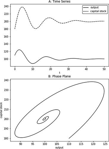
As discussed in Section 2, a necessary condition for oscillations in this type of model is that $J_{12}$ and $J_{21}$ have opposite signs, which in the Phillips model is satisfied when $a>0,$ $\beta >0,$ and $v>0.$ A simulated time path of the Phillips model with stable oscillations is presented in Figure 1. The business cycle illustrated in this figure proceeds as follows: an initial increase in output at a low level of capacity leads to further increases in output and capacity. The induced increase in capacity dampens further increases in output and capacity, leading to a turning point in output when the level of capacity with respect to output is sufficiently high. In the ensuing recession, falling output induces dis-investment, until the level of capacity with respect to output is sufficiently low that capacity accumulation recovers and a boom sets in. In its essential aspects, this business cycle mechanism is “a simple consequence of the one omnipresent, incontestable dynamic fact in economics - the necessity to have both stocks and flows of goods” (Goodwin 1951, p. 3).

Figure 1. Simulated time path of the multiplier-accelerator model in (4(4) $$\dot{Y}=a\left(c+\beta v-1\right)Y-a\beta K+aA,$$(4) ) and (5(5) $$\dot{K}=\beta \left(vY-K\right).$$(5) ), with parametrisation $a=0.6, \beta =0.6, v=2, c=0.5, A=50.$

There are a number of extensions to the basic multiplier-accelerator model. In particular, business cycle theorists working from the 1930s to the 1950s were dissatisfied with the limitations of linear models and sought to explain endogenous fluctuations by the use of non-linearities. Early examples are the discursive theory presented in Kaldor (1940), and the ceiling model introduced in Hicks (1950), where output is limited above by a resource constraint. Similar arguments are presented in Goodwin (1951) and Morishima (1958). The key difference between the linear and nonlinear versions of the model is that the latter can generate limit cycles in $Y$ and $K.$ They do this, in general, not by changing the sign structure of the off-diagonal elements, but by changing the sign structure of the on-diagonal elements. Specifically, the non-linearities tend to be such that the on-diagonal elements induce unstable dynamics near the steady state, and stable dynamics away from the steady state, although this is often not quite so obvious in discrete time models.

Non-linear multiplier-accelerator models have been studied in a large number of papers. For example, Szydłowski and Krawiec (2001) provide a Kaldor-Kalecki time delay differential equation model with a delay in the capital accumulation equation, and Puu, Gardini, and Sushko (2005) develop a Hicksian multiplier-accelerator model with a time-varying floor on the depreciation rate. Reformulating Samuelson (1939), Westerhoff (2006b) introduces nonlinearities via agents who follow a combination of extrapolative and regressive expectation formation rules to predict growth fluctuations, which is related to the models discussed in section 5 of this paper. This is a good example of a discrete time non-linear model in which the mechanism by which the non-linearity induces limit cycles is not obvious without numerical simulation. A history of multiplier-accelerator models can be found in Heertje and Heemeijer (2002).

4. The Goodwin model

The Goodwin model was first published in Goodwin (1967). The model is a “starkly schematized” formalization of a simple Marxian profit-led system, drawing on Marx’s fragmentary accounts of industrial cycles in Capital. Thus,

“The course characteristic of modern industry, viz., a decennial cycle (interrupted by smaller oscillations), of periods of average activity, production at high pressure, crisis and stagnation, depends on the constant formation, the greater or less absorption, and the re-formation of the industrial reserve army or surplus-population … Taking them as a whole, the general movements of wages are exclusively regulated by the expansion and contraction of the industrial reserve army, and these again correspond to the periodic changes of the industrial cycle.” (Marx 1867 [1967], pp. 592–596).

In Goodwin’s formalization of this theory, rising employment rates lead to an increase in the labor share of income, via a real wage Phillips curve. During the boom phase of the cycle the rise in employment increases the bargaining power of workers, which results in higher wages and lower profits. As profitability declines, capital accumulation declines, which leads to a decrease in the employment rate as a recession sets in. Eventually, rising unemployment leads to a decrease in the labor share of income, a recovery in profits, and a consequent increase in accumulation.

Goodwin’s original model was a classical model where Say’s law was operational. Firms always produce at full capacity and all output is sold. However, in the course of the 1980s and 1990s, what we will refer to as neo-Goodwin models were developed which are formulated in a Keynesian setting with flexible capacity utilization (Barrales-Ruiz et al. 2022 provide a review of this literature). These models replace the assumption that all profits are re-invested with the assumption of a profit-led demand regime. Unlike the multiplier-accelerator model, the Goodwin model has always been a recognizably heterodox model and continues to be used extensively and developed within the Marxist research community. However, it is not a model that all heterodox economists would agree with, as attested to by the extensive literature on wage-led versus profit-led growth (see Lavoie 2017 for a historical overview of this literature).

While the multiplier-accelerator model studies cycles arising from the interaction of output and capacity, the original Goodwin model assumes away variable capacity utilization. Say’s law holds, firms produce at full capacity and all output is sold. Instead, it studies cycles arising from the interaction of the employment rate and income distribution. Denoting the real wage by $w$ and the employment rate by $v,$ the labor market is characterized by a real wage Phillips curve as follows, (8) $$\frac{\dot{w}}{w}=-\gamma +\rho v,$$(8) where $\gamma >0$ and $\rho >0.$ Real wage growth is thus increasing in the employment rate, which reflects a bargaining theory of wage determination where existing workers’ outside options are directly affected by the probability of finding an alternative job.

To determine the employment rate, assume that output $Y$ is determined by the existing capital stock $K$ given a fixed capital output ratio $\sigma ,$ and that labor productivity is constant and given by $Y/L=a.$ If total profits are entirely accumulated as capital, we have, (9) $$\frac{\dot{Y}}{Y}=\frac{\dot{K}}{K}=\frac{1-\frac{w}{a}}{\sigma },$$(9) i.e., the rate of accumulation and therefore the rate of output growth is equal to the rate of profit. If we then assume that labor productivity grows at rate $\alpha ,$ and that the total working population grows at rate $\beta ,$ the growth of the employment rate is a linear function of the rate of profit, (10) $$\frac{\dot{v}}{v}=\frac{1-\frac{w}{a}}{\sigma }-(\alpha +\mathrm{\beta }).$$(10)

Finally, denote the labor share as $w/a=u.$ We then have the two-dimensional business cycle model, (11) $$\dot{v}=\left[\frac{1-u}{\sigma }-\left(\alpha +\mathrm{\beta }\right)\right]v,$$(11) (12) $$\dot{u}=\left[-\left(\alpha +\gamma \right)+\rho v\right]u.$$(12)

The Jacobian for the system described by (11(11) $$\dot{v}=\left[\frac{1-u}{\sigma }-\left(\alpha +\mathrm{\beta }\right)\right]v,$$(11) ) and (12(12) $$\dot{u}=\left[-\left(\alpha +\gamma \right)+\rho v\right]u.$$(12) ) is as follows, (13) $$J=\left[\begin{array}{cc}0& -\frac{v^{*}}{\sigma }\\ \rho u^{*}& 0\end{array}\right],$$(13)

Where $v^{*}=(\alpha +\gamma )/\rho$ is the equilibrium employment rate, and $u^{* }=1-\sigma \left(\alpha +\beta \right)$ is the equilibrium labor share. As the capital-output ratio is positive by definition, and we have already assumed $\rho >0,$ the Jacobian has the following sign structure, (14) $$\mathit{sgn}\left(J\right)=\left[\begin{array}{cc}0& -\\ +& 0\end{array}\right].$$(14)

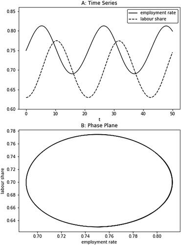
As the necessary condition for cycles exists, and the trace is zero, the equilibrium is a center and marginally stable oscillations exist.⁴ An example of the dynamics generated by the Goodwin model are presented in Figure 2. The business cycle in this figure proceeds as follows: an increase in the employment rate from the trough of a recession leads to a steady increase in workers’ bargaining power, which leads to an upturn in the labor share. As the labor share increases, the rate of profit declines, which leads to a decrease in capital accumulation. This eventually leads to a decline in the employment rate as a recession sets in.

Figure 2. Simulated time path of the Goodwin model in (11) and (12), with parametrisation $\alpha =0.05, \beta =0.05, \sigma =3, \rho =0.5, \gamma =0.325.$

As with the multiplier-accelerator model, there are a number of extensions to the basic Goodwin model. Harvie, Kelmanson, and Knapp (2007) and Desai et al. (2006) address an important shortcoming of the original Goodwin (1967) model, which is that the wage share and the employment rate can exceed unity. These restrictions lead to more complex solutions, but the model still exhibits similar predator-prey Goodwin cycles. Notably, the trajectories of the employment rate and labor share can exhibit significant asymmetry in these models whenever the equilibria are close to their upper or lower bounds, as both the employment rate and labor share are limited to the unit square.

Desai (1973) and Velupillai (1979) relax Goodwin’s assumption of a fixed capital-output ratio and study the dynamic properties of such models with varying capital-output ratios. Desai (1973) introduces varying capacity utilization (proxied by employment), and actual and anticipated inflation. When workers are not able to adjust their wage demands to actual wage inflation, then inflation has a stabilizing effect. Inasmuch as inflation is considered important in heterodox business cycle theory, it is generated via a conflict process and affects aggregate demand via its effect on the income distribution. More recently, Tavani and Zamparelli (2015) have incorporated endogenous technical change into the standard Goodwin model. These examples only touch upon a very extensive literature, overviews of which can be found in Veneziani and Mohun (2006) and Barrales-Ruiz et al. (2022).

5. The Minsky model

Hyman Minsky proposed his financial instability hypothesis in Minsky (1975, 1986 [2008]), building on the debt deflation theory of Fisher (1933), the theories of credit and banking of Schumpeter (1934, 1939), and the macroeconomic theory of Keynes (1936). One of the key mechanisms that underlies Minsky’s theory of capitalist fluctuations is the endogenous move from financially robust corporate balance sheets, in which profits cover debt service and new investment, to financially fragile corporate balance sheets, in which profits do not cover debt service and new investment, and new debt has to be issued. In the boom phase of the cycle firms become more optimistic, thus, their desired investment rate rises faster than retained profits. To cover that gap, firms increase their debt ratios. As the debt ratios of firms increase, their debt service commitments rise accordingly, increasing their overhead costs. Eventually, the rise in debt service commitments makes investment unsustainable, hence a slowdown in investment occurs, triggering a recession.

Different from the multiplier-accelerator model and the Goodwin model, there is no canonical Minsky model, but a number of competing formalisations of Minsky’s business cycle theory. Nikolaidi and Stockhammer (2017), in a recent survey, present no fewer than eight families of Minsky models and we make no pretense of covering all of them. Minsky’s own work on the subject tended to emphasize explosive multiplier-accelerator mechanisms with financial conditions (particularly borrowers’ risk perceptions) determining the ceiling to continued expansion (Minsky 1957, 1959; Ferri and Minsky 1992; Delli Gatti, Gallegati, and Gardini 1994). Formalisations by other authors differ in a number of important respects, including the emphasis on debt stocks versus asset prices, the importance of interest rates, and whether limit cycles, secular collapses, and/or multiple steady states are studied. In what follows, we present a simplified version of a formal Minsky model due to Asada (2001, 2012), which fits neatly with our general approach outlined in section 2.⁵

Asada (2001, 2012) proposes a similar output adjustment mechanism to the Phillips (1954) model considered in section 3. Denoting the ratio of output $Y$ to capital $K$ by $y,$ consumption $C$ to capital by $c,$ and investment $I$ to capital by $h,$ we have, (15) $$\dot{y}=a(c+h-y),$$(15) which is analogous to (1(1) $$\dot{Y}=a\left(C+I+A-Y\right),$$(1) ) above. Kalecki’s principle of increasing risk (Kalecki 1937) is used to determine the level of investment. Denoting the marginal efficiency of investment by $m,$ the interest rate by $i,$ and a measure of the “marginal risk” of an extra unit of investment by $\sigma ,$ investment will be increased until $m=i+\sigma .$

If we ignore adjustment costs and depreciation, then the growth rate of the capital stock is given by $h.$ Asada supposes that the marginal efficiency of investment is a function of both $h$ and the rate of profit $r,$ and that the “marginal risk” of an extra unit of investment is a function of $h,$ $r,$ $i,$ and the debt to capital ratio $d$ (plus an exogenous limit on retained profits, which we omit). Thus, the optimal level of investment is given by the solution to, (16) $$m\left(h,r\right)=i+\sigma (h,r,i,d),$$(16) from which we have a general investment function with a debt effect, (17) $$h=h(r,i,d).$$(17)

In order to derive the reduced form equation of motion in output, suppose that the profit share is fixed and denoted by $\varsigma ,$ so $r=\varsigma y.$ Without loss of generality, assume that consumption is equal to labor income, which is the same assumption used in the Goodwin model in section 4, and $c=(1-\varsigma )y.$ Substitution, using (15) and (17), yields the equation of motion for output, (18) $$\dot{y}=a\left(h\left(y,i,d\right)-\varsigma y\right).$$(18)

Turning next to the equation of motion for debt, we rely on a simple budget equation for the firm sector given by, (19) $$\dot{D}=hK-s(rK-iD),$$(19) where $D$ denotes the debt stock and $s$ denotes firms’ profit retention rate. Noting that, $$\frac{\dot{d}}{d}=\frac{\dot{D}}{D}-\frac{\dot{K}}{K}=\frac{\dot{D}}{D}-h,$$ and having assumed a constant profit share, we have the reduced form equation of motion for debt, (20) $$\dot{d}=h\left(y,i,d\right)-s\left(\varsigma y-id\right)-h\left(y,i,d\right)d.$$(20)

This Minsky model is then made up of the reduced form equation in the output to capital ratio (18) and the reduced form equation in the debt to capital ratio (20). Thus, the Jacobian for the system described by (18) and (20) is as follows, (21) $$J=\left[\begin{array}{cc}a(h_y-\varsigma )& a{h}_d\\ h_y\left(1-d^{*}\right)-s\varsigma & h_d\left(1-d^{*}\right)+si\end{array}\right],$$(21) where $h_y$ and $h_d$ denote the partial derivative of $h$ with respect to $y$ and $d$ evaluated at the steady state, respectively, and $d^{*}$ denotes the steady state debt to capital ratio. To gain insight into the sign structure of this Jacobian, further restrictions are imposed. We impose the following conditions: investment is increasing in the level of output ($h_y>0$) and decreasing in the level of debt ($h_d<0$); the solvency condition $d^{*}<1$ states that equilibrium value of debt is less than the equilibrium value of the capital stock; and finally, $h_y\left(1-d^{*}\right)>s\varsigma$ states that firms take on debt to fund investment expenditure. Given these assumptions, we arrive at the following Jacobian sign structure. (22) $$\mathit{sgn}\left(J\right)=\left[\begin{array}{cc}?& -\\ +& ?\end{array}\right].$$(22)

The signs of the off-diagonal elements, implying that increases in output lead to increases in debt, and increases in debt subsequently induce decreases in output, are standard in the Minskyan literature. The signs of the main diagonal elements, however, differ between the varieties of Minskyan business cycle models. Asada (2001, 2012) assumes an explosive (or Kaldorian) output market, with stabilizing own-effects of the debt stock. This mechanism is proposed in a number of papers, notably Foley (1987). However, one could assume stabilizing own-effects of output with an explosive debt dynamic (as in Charles (2008), Fazzari et al. (2008), Lima and Meirelles (2006), and Nishi (2012)) with the main cyclical mechanism remaining the same.

A business cycle expansion in our Minskyan model involves investment expenditure increasing beyond retained profits, as firms explicitly or implicitly reduce their margins of safety. As a result, the debt stock increases. However, as the debt stock continues to increase, it acts as a drag on investment, either directly (through increased interest payments reducing retained profits), or indirectly (through increases in perceived risk). The resulting decline in investment leads to a decline in output as a recession sets in. The dynamics of a linearized version of this model will be qualitatively identical to the multiplier-accelerator dynamics in Figure 1, with the capital stock replaced by the debt stock. In fact, we could paraphrase Goodwin’s 1951 observation of the multiplier-accelerator model and observe that our Minskyan business cycle mechanism is, ‘a simple consequence of the other omnipresent, incontestable dynamic fact in economics - the necessity to have both stocks and flows of debt’.

There are, again, several extensions to the basic model. The model described by (18(18) $$\dot{y}=a\left(h\left(y,i,d\right)-\varsigma y\right).$$(18) ) and (20(20) $$\dot{d}=h\left(y,i,d\right)-s\left(\varsigma y-id\right)-h\left(y,i,d\right)d.$$(20) ) is non-linear, even when the investment function is linear, and can undergo a Hopf bifurcation as the eigenvalues of $J$ move across the imaginary axis (Asada 2001, pp. 81–83). Further non-linearities can exist if the interest rate on debt is specified as a function of debt. This is quite common in the literature, with Asada (2001) specifying the interest rate as an increasing function of the debt to capital ratio. Charles (2008) considers a linear (positive) function of the interest rate. The earlier model of Keen (1995) considers a similar function in the debt to output ratio. This type of interest rate function adds higher order polynomial terms in the equation of motion for debt, raising the possibility of multiple equilibria and a variety of complex dynamics. This type of model has been used to consider secular breakdowns, the coexistence of stable and unstable steady states, and chaotic dynamics, with two notable examples including the models of Semmler (1987) and Franke and Semmler (1989).

What distinguishes Minskyan models with endogenous interest rates from the simple debt cycle models is that a crisis may also occur because of a policy decision by the central bank, or due to legislation change about the use of reserves, and not necessarily by business debt accumulation itself alone.⁶ Minsky did in fact indicate that he considered rising interest rates to be important in the onset of a recession (e.g., Minsky (1986 [2008], p. 239). However, as demonstrated above, a variable interest rate is not necessary for the existence of business cycles driven by the interaction of output and the stock of debt, and simple Minsky models can therefore be specified with the interest rate held constant, as in our model and the model in Nishi (2012).

6. Momentum trader models

Our final family of business cycle models is the family of speculative asset pricing models that emerge from the interaction of different types of traders. This approach is closely associated with behavioral economics, which posits that economic agents are not necessarily substantively rational, but follow simple behavioral heuristics that can amount to a type of procedural rationality. In the context of financial markets, one well-known distinction is between momentum traders (a type of chartist), who form extrapolative expectations based on past asset prices, and fundamentalists, who form price expectations based on non-price information (such as underlying profitability).

Two clarifications are required. First, strictly speaking the momentum trader model is a theory of the financial cycle rather than the business cycle. However, as adding a consumption function with a wealth effect or an investment function with Tobin’s $q$ will easily turn a financial cycle into a business cycle, we will treat these theories as business cycle theories. Second, momentum trader models are usually associated with behavioral economics, which sits at a borderline of mainstream and heterodox economics. As discussed in the introduction, however, we take a very wide approach to our definition of heterodoxy, and the financial instability formalized in these models is very close in spirit to discursive approaches that can be found in thinkers such as Kindleberger and Minsky.

An important early example of a momentum trader model is Beja and Goldman (1980). The model includes two types of financial market traders: fundamentalists and chartists. Fundamentalists have relatively long time horizons, and adjust their demand for assets based on the divergence between the current price and its fundamental value. They consider expected income streams rather than capital gains, and expect actual asset prices to revert to their fundamental value (eventually). Chartists have comparatively short time horizons, and attempt to take advantage of extrapolated price changes. They consider past price movements, not fundamental values. A distinguishing feature of the momentum trader model is, therefore, the central role of expectation formation in driving economic dynamics, and the importance of heterogeneity in this respect. Following Franke’s (2009, p. 1336) formulation of the Beja and Goldman (1980) model, the demand functions of fundamentalist and chartist traders can be written as follows, (23) $$d^f=\phi \left(v-p\right),$$(23) (24) $$d^c=\chi \pi ,$$(24) where $d^f$ is the demand for assets by fundamentalists, $d^c$ is the demand for assets by chartists, $p$ is the log price, $v$ is the fundamental value of the asset, and $\pi$ is chartists’ current perception of price trends. The coefficients $\phi$ and $\chi$ represent the responsiveness of fundamentalist and chartist demand to their respective ‘signals’ (note that, if the asset is overvalued then fundamentalists sell it, and vice versa). Franke (2009) specifies the rates of changes of $p$ and $\pi ,$ as follows, (25) $$\dot{p}={\beta }_p(d^f+d^c),$$(25) (26) $$\dot{\pi }={\beta }_{\pi }(\dot{p}-\pi ),$$(26) where ${\beta }_p$ is a positive coefficient, and ${\beta }_{\pi }$ is the adjustment speed of chartists’ perception of price trends. After substituting Equations (23)(23) $$d^f=\phi \left(v-p\right),$$(23) , (24)(24) $$d^c=\chi \pi ,$$(24) into (25(25) $$\dot{p}={\beta }_p(d^f+d^c),$$(25) ) and (26(26) $$\dot{\pi }={\beta }_{\pi }(\dot{p}-\pi ),$$(26) ), we arrive at the following two-dimensional system, (26) $$\dot{p}={\beta }_p\left(\phi \right(v-p)+\chi \pi ),$$(26) (27) $$\dot{\pi }={\beta }_{\pi }\left[{\beta }_p\phi \right(v-p)-({\beta }_p\chi -1\left)\pi \right].$$(27)

Thus, the Jacobian for the system described by (26(26) $$\dot{p}={\beta }_p\left(\phi \right(v-p)+\chi \pi ),$$(26) ) and (27(27) $$\dot{\pi }={\beta }_{\pi }\left[{\beta }_p\phi \right(v-p)-({\beta }_p\chi -1\left)\pi \right].$$(27) ) is as follows, (28) $$J=\left[\begin{array}{cc}{-\beta }_p\phi & {\beta }_p\chi \\ -{\beta }_{\pi }{\beta }_p\phi & {-{\beta }_{\pi }(\beta }_p\chi -1)\end{array}\right],$$(28) which has off-diagonal elements of opposite sign whenever ${\beta }_p,\mathrm{ }\chi ,\mathrm{ }\phi ,{\beta }_{\pi }>0,$ all of which are intuitive restrictions on the parameter space. Thus, this type of model satisfies our basic framework.

The intuition of this momentum trader cycle is as follows. During a boom, momentum traders expect asset price inflation to continue and thus fuel further price increases. Fundamentalists constitute the dampening force and put a downward pressure on prices. As the boom peters out, momentum traders lower their expectations for further price growth and eventually a turning point occurs. In the downturn momentum traders contribute to the overshooting of prices and thus the financial crisis. There is thus an interplay between different types of agents; if momentum trader demand outweighs fundamentalist demand, then asset prices will rise, and this type of asset price inflation will continue until fundamentalist demand outweighs that of momentum traders. If consumption is a simple function of asset prices, and/or investment a simple function of Tobin’s $q,$ then the momentum trader financial cycle will ‘drag along’ the real economy (in a similar manner to the distribution cycles in the pseudo-Goodwin cycles of Stockhammer and Michell (2017)).

Dynamics of this basic form have also been introduced into behavioral versions of the New Keynesian model. Paul De Grauwe, for example, has presented a series of papers in which cyclical fluctuations arise (or are exacerbated) by adaptive learning of strategies that resemble fundamentalist and extrapolative expectations (De Grauwe 2011). De Grauwe and Kaltwasser (2012), for example, apply this approach to foreign exchange markets, and show that endogenous cycles in exchange rates can emerge. De Grauwe (2012) is a useful overview, and includes simple models for closed economies. A similar sequence of papers within the New Keynesian literature builds on Branch and McGough (2009, 2010), which in turn rely heavily on the type of strategy switching introduced to (partial) equilibrium models in Brock and Hommes (1997). In the latter paper, firms operating within a cobweb model framework have the choice of a low quality predictor at zero cost, or a high quality predictor at positive cost, and changes in the proportion of firms using each predictor can induce highly complex dynamics. A review of the behavioral New Keynesian literature as a whole can be found in Calvert Jump and Levine (2019).

These speculative mechanisms also play a role in some Minsky models, and form a distinct family of Minsky models in the review of Nikolaidi and Stockhammer (2017). But despite Minsky’s emphasis on the role of asset price inflation for economic activity, and the existence of a considerable literature on momentum trader models, the formal Minskyan literature examining the role of asset price dynamics is considerably smaller than the literature discussing debt and indebtedness. Ryoo (2013, 2016) is an example of a Minsky model that discusses momentum trader dynamics, and Ryoo (2016) presents a Keynesian macro model where house prices are derived from momentum trader models and feed into consumption of credit constraint households.

7. Discussion

Sections 3, 4, 5 and 6 have examined four distinct heterodox theories of the business cycle. All four are logically coherent, have a prima facie plausibility, can be formally modeled, and can be used to demonstrate the possibility of recurring cycles. We have argued that each business cycle theory can be understood as having stabilizing and destabilizing forces that interact. The four theories differ in where they locate these forces, which we summarize in Table 1. The multiplier-accelerator theory has both the stabilizing and destabilizing forces located in the goods market; the Goodwin model has the destabilizing force in the goods market and the stabilizing force in the labor market; the Minskyan model has the destabilizing force in the goods market and the stabilizing force in the financial markets; while the momentum trader model has both stabilizing and destabilizing forces located in the financial markets.

Table 1. Overview of the stabilizing and destabilizing forces in different heterodox business cycle theories (d denotes destabilizing; s denotes stabilizing).

	Goods markets	Labor market	Financial markets
Multiplier-accelerator	d, s
Goodwin	d	s
Minsky	d		s
Momentum trader			d, s

A key question is whether these theories are competing, or whether they are complementary. We argue that the theories are substantially competing, but theoretically consistent. The theories are substantially competing as they identify different mechanisms that drive the business cycle: for any given business cycle or set of business cycles, they offer alternative explanations. However, they are clearly not mutually exclusive; the different mechanisms could coexist at different points in time, space, and/or at different frequencies. In other words, the multiplier-accelerator, Goodwin, Minsky, and momentum trader mechanisms could coexist in different decades within the same country, different countries at the same point in time, and some could drive longer frequency cycles while others could drive shorter frequency cycles.

We also argue that the four theories are theoretically consistent, and that it ought to be possible to construct a model that encompasses all of them. First, whereas mainstream business cycle accounts focus primarily on the identification of different shocks that drive fluctuations at different periods in time, this method would focus on the different mechanisms that propagate those shocks at different periods in time, providing both a heterodox complement and competitor to mainstream business cycle theory. Second, the common denominator within heterodox business cycle models is the presupposition of a common form of behavior based on animal spirits and adaptive learning. Multiplier-accelerator, Goodwin and Minsky models apply this type of behavior to business investment decisions; momentum trader models apply it to asset prices. A strength of the momentum trader models is that they make the behavioral assumptions explicit. They posit (for the momentum traders) a behavioral rule that projects past experience forward and thus creates overshooting. While often not explicit, this assumption also applies to household and business behavior in the other three models, where it is usually subsumed into a measure of ‘autonomous’ demand.

Unfortunately, there is a notable lack of communication between the different streams of heterodox business cycle theory. Progress has been made within each stream, but rarely by contrasting arguments with other theories or by incorporating elements of alternative theories. This reflects a more general pattern in heterodox economics, which tends to form segmented niches that refer to mainstream economics much more than to other heterodox approaches (Kapeller and Dobusch 2012; Glötzl and Aigner 2018). We argue that this is a major shortcoming, and that there is need for a synthesis. There are pitfalls in proceeding separately: focusing on a single business cycle mechanism at a time may lead to the misinterpretation of actual economies, in particular once the models are applied to data. Notably, as demonstrated in Stockhammer and Michell (2017), some business cycle models can generate data that seemingly confirm the predictions of a completely different model. Specifically, by appending a reserve-army distribution equation to a Minskyan model, they demonstrate that pseudo-Goodwin cycles in output and the labor share can be generated. Of course, this argument could be applied to all sorts of models; one can easily imagine appending an asset-pricing equation to a multiplier-accelerator model, for example, to yield pseudo-Minsky cycles.

That such a synthesis is possible is suggested by the existing examples of synthetic heterodox business cycle models, including Taylor (2012), who takes as his starting point the Harrodian instability of investment expenditure, and suggests that either distributional dynamics (following Goodwin) or equity prices and debt stocks (following Minsky) can stabilize the economy. His models are based on the general approach of Flaschel (2009), who – with various coauthors including Matthieu Charpe, Reiner Franke, Carl Chiarella, Christian Proano and Willi Semmler – has discussed a large number of models that synthesize Marxian, Keynesian and Schumpeterian dynamics. Another example of the synthetic approach to heterodox business cycle theory can be found in Yilmaz and Stockhammer (2019), who present a framework that nests a pure multiplier accelerator model and a pure Minskyan model.

While we assert, therefore, that such a synthesis model is possible, and that heterodox economists should work toward such a model, we do not claim that heterodox economists will be able to agree on the model. Ideally, such an exercise would provide a common language in which all of the major causal mechanisms are represented, to permit a simple vehicle through which theoretical and empirical disagreements can be easily expressed. Rather than a general consensus, our point is that of a common analytical framework that allows constructive conversation between heterodox streams, shifts the focus of heterodox macroeconomics onto empirical specification and identification, and overcomes the negative fixation with mainstream economics.

Acknowledgements

We would like to thank Giorgos Gouzoulis for his assistance with earlier drafts of this paper, Romar Correa for very helpful corrections, and the editor and referees. Any remaining errors are the responsibility of the authors.

Additional information

Notes on contributors

Robert Calvert Jump

Robert Calvert Jump, University of Greenwich, School of Accounting, Finance and Economics, Greenwich SE10 9LS. Email: [email protected]

Engelbert Stockhammer

Engelbert Stockhammer, King's College London, Department of European and International Studies, Virginia Woolf Building, 22 Kingsway, London WC2B 6LE. E-mail: [email protected]

Notes

1 Typical examples include Real Business Cycle model (Kydland and Prescott 1982) and the workhorse New Keynesian model (Woodford 2003, Gali 2008).

2 If we restrict our enquiry to the basic macroeconomic aggregates, including output growth, capital formation, income shares, employment rates, private debt growth, and asset price growth, then a basic stylised fact is near-stationarity in the majority of empirical time series. In particular, non-stationary macroeconomic series tend to be rendered stationary after first differencing or the removal of a polynomial trend.

3 Instead of (2(2) $$\dot{Y}=a\left(\dot{K}+A-(1-c)Y\right).$$(2) ) an alternative specification for output is used in Goodwin (1951), where the output market is assumed to be in temporary equilibrium at all points in time, so $Y = C + I + A.$ If we combine this with the “dynamic multiplier”, $C=cY-\epsilon \dot{Y}$ we have $\dot{Y}={\epsilon }^{-1}(\dot{K̇}+A-(1-c)Y).$ The reduced form is identical to (2(2) $$\dot{Y}=a\left(\dot{K}+A-(1-c)Y\right).$$(2) ) aside from the change in parameters, but the implied behaviour of inventories will differ.

4 As ${\left(J_{11}-J_{22}\right)}^2=0$ in the Goodwin model, then ${\left(J_{11}-J_{22}\right)}^2<\left|4J_{12}{J}_{21}\right|$ in the system made up of (11(11) $$\dot{v}=\left[\frac{1-u}{\sigma }-\left(\alpha +\mathrm{\beta }\right)\right]v,$$(11) ) and (12(12) $$\dot{u}=\left[-\left(\alpha +\gamma \right)+\rho v\right]u.$$(12) ). The determinant of the Jacobian is given by $\mathrm{\Delta }=\rho v^{*}{u}^{*}/\sigma$ in the Goodwin model, which is positive under the assumptions provided.

5 This would qualify as a Kaldor-Minsky model in Nikolaidi and Stockhammer’s classification.

6 Minsky (1986, p. 86) himself argues that such a crisis is plausible, highlighting two events in the post-War US economy, in which inflation targeting-oriented monetary policy led to such a recession (ibid., pp. 73, 102).

References

- Aikman, D., A. G. Haldane, and B. D. Nelson. 2015. “Curbing the Credit Cycle.” The Economic Journal 125 (585):1072–109.
- Arnold, L. 2002. Business Cycle Theory. Oxford: Oxford University Press.
- Asada, T. 2001. “Nonlinear Dynamics of Debt and Capital: A Post-Keynesian Analysis.” In Evolutionary Controversies in Economics, edited by Y. Aruka. Tokyo: Springer Japan.
- Asada, T. 2012. “Modeling Financial Instability.” European Journal of Economics and Economic Policies 9 (2):215–32. doi: 10.4337/ejeep.2012.02.06.
- Barrales‐Ruiz, J., I. Mendieta‐Muñoz, C. Rada, D. Tavani, and R. Von Arnim. 2022. “The Distributive Cycle: Evidence and Current Debates.” Journal of Economic Surveys 36 (2):468–503.
- Beaudry, P., D. Galizia, and F. Portier. 2020. “Putting the Cycle Back into Business Cycle Analysis.” American Economic Review 110 (1):1–47.
- Beja, A., and M. B. Goldman. 1980. “On the Dynamic Behavior of Prices in Disequilibrium.” The Journal of Finance 35 (2):235–48. doi: 10.1111/j.1540-6261.1980.tb02151.x.
- Bernard, L., A. V. Gevorkyan, T. I. Palley, and W. Semmler. 2014. “Time Scales and Mechanisms of Economic Cycles: A Review of Theories of Long Waves.” Review of Keynesian Economics 2 (1):87–107.
- Borio, C. 2014. “The Financial Cycle and Macroeconomics: What Have we Learnt?” Journal of Banking & Finance 45:182–98.
- Branch, W. A., and B. McGough. 2009. “A New Keynesian Model with Heterogeneous Expectations.” Journal of Economic Dynamics and Control 33 (5):1036–51.
- Branch, W. A., and B. McGough. 2010. “Dynamic Predictor Selection in a New Keynesian Model with Heterogeneous Expectations.” Journal of Economic Dynamics and Control 34 (8):1492–508.
- Brock, W. A., and C. H. Hommes. 1997. “A Rational Route to Randomness.” Econometrica 1997:1059–95.
- Calvert Jump, R., and P. Levine. 2019. “Behavioural New Keynesian Models.” Journal of Macroeconomics 59:59–77.
- Charles, S. 2008. “Teaching Minsky’s Financial Instability Hypothesis: A Manageable Suggestion.” Journal of Post Keynesian Economics 31 (1):125–38. doi: 10.2753/PKE0160-3477310106.
- Delli Gatti, D., M. Gallegati, and L. Gardini. 1994. “Complex Dynamics in a Simple Macroeconomic Model with Financing Constraints.” In New Perspectives in Monetary Macroeconomics, edited by G. Dymski, and R. Pollin. Michigan: Michigan University Press.
- De Grauwe, P. 2011. “Animal Spirits and Monetary Policy.” Economic Theory 47 (2–3):423–57. doi: 10.1007/s00199-010-0543-0.
- De Grauwe, P. 2012. Lectures on Behavioral Macroeconomics. Princeton: Princeton University Press.
- De Grauwe, Paul, and Pablo Rovira Kaltwasser. 2012. “Animal Spirits in the Foreign Exchange Market.” Journal of Economic Dynamics and Control 36 (8):1176–92. doi: 10.1016/j.jedc.2012.03.008.
- Desai, M. 1973. “Growth Cycles and Inflation in a Model of the Class Struggle.” Journal of Economic Theory 6 (6):527–45. doi: 10.1016/0022-0531(73)90074-4.
- Desai, M., B. Henry, A. Mosley, and M. Pemberton. 2006. “A Clarification of the Goodwin Model of the Growth Cycle.” Journal of Economic Dynamics and Control 30 (12):2661–70. doi: 10.1016/j.jedc.2005.08.006.
- Fazzari, S., P. Ferri, and E. Greenberg. 2008. “Cash Flow, Investment, and Keynes–Minsky Cycles.” Journal of Economic Behavior & Organization 65 (3–4):555–72.
- Ferri, P., and H. P. Minsky. 1992. “Market Processes and Thwarting Systems.” Structural Change and Economic Dynamics 3 (1):79–91. doi: 10.1016/0954-349X(92)90027-4.
- Fisher, I. 1933. “The Debt-Deflation Theory of Great Depressions.” Econometrica 1 (4):337–57. doi: 10.2307/1907327.
- Flaschel, P. 2009. The Macrodynamics of Capitalism: Elements for a Synthesis of Marx, Keynes, and Schumpeter. Berlin: Springer-Verlag.
- Foley, D. K. 1987. “Liquidity-Profit Rate Cycles in a Capitalist Economy.” Journal of Economic Behavior & Organization 8 (3):363–76. doi: 10.1016/0167-2681(87)90050-3.
- Franke, R. 2009. “A Prototype Model of Speculative Dynamics with Position-Based Trading.” Journal of Economic Dynamics and Control 33 (5):1134–58. doi: 10.1016/j.jedc.2009.01.006.
- Franke, R. and Semmler, W. 1989. Debt Financing of Firms, Stability and Cycles in a Dynamical Macroeconomic Growth Model. Business Cycles: Theory and Empirical Methods. London: Kluwer.
- Gabisch, G., and H. Lorenz. 1987. “Business Cycle Theory.” Lecture Notes in Economics and Mathematical Systems. Berlin: Springer-Verlag.
- Gali. 2008. Monetary Policy, Inflation, and the Business Cycle: An Introduction to the New Keynesian Framework and Its Applications. Princeton: Princeton University Press.
- Glötzl, F., and E. Aigner. 2018. “Orthodox Core–Heterodox Periphery? Contrasting Citation Networks of Economics Departments in Vienna.” Review of Political Economy 30 (2):210–40. doi: 10.1080/09538259.2018.1449619.
- Goodwin, R. M. 1951. “The Nonlinear Accelerator and the Persistence of Business Cycles.” Econometrica 19 (1):1–17. doi: 10.2307/1907905.
- Goodwin, R. M. 1967. “A Growth Cycle.” In Socialism, Capitalism and Economic Growth: Essays Presented to Maurice Dobb, edited by C. H. Feinstein. Cambridge: Cambridge University Press.
- Harvie, D., M. A. Kelmanson, and D. G. Knapp. 2007. “A Dynamical Model of Business Cycle Asymmetries: Extending Goodwin.” Economic Issues 12 (1):53–72.
- Heertje, A., and P. Heemeijer. 2002. “On the Origin of Samuelson’s Multiplier-Accelerator Model.” History of Political Economy 34 (1):207–18. doi: 10.1215/00182702-34-1-207.
- Hicks, J. R. 1950. A Contribution to the Theory of the Trade Cycle. Oxford: Clarendon Press.
- Hohnisch, M., and F. H. Westerhoff. 2007. “A Note on Interactions-Driven Business Cycles.” Journal of Economic Interaction and Coordination 2 (1):85–91. doi: 10.1007/s11403-006-0017-4.
- Kaldor, N. 1940. “A Model of the Trade Cycle.” The Economic Journal 50 (197):78–92. doi: 10.2307/2225740.
- Kalecki, M. 1933 [1990]. “Stimulating the Business Upswing.” In Collected Works of Michał Kalecki Volume I Capitalism: Business Cycles and Full Employment, edited by J. Osiatyński. Oxford: Clarendon Press.
- Kalecki, M. 1935. “A Macroeconomic Theory of the Business Cycle.” Econometrica 3 (3):327–44. doi: 10.2307/1905325.
- Kalecki, M. 1937. “The Principle of Increasing Risk.” Economica 4 (16):440–7. doi: 10.2307/2626879.
- Kalecki, M. 1954. Theory of Economic Dynamics, London, Allen & Unwin.
- Kapeller, J., and L. Dobusch. 2012. “A Guide to Paradigmatic Self-marginalization - Lessons for post-Keynesian Economists.” Review of Political Economy 24 (3):469–87. doi: 10.1080/09538259.2012.701928.
- Keen, S. 1995. “Finance and Economic Breakdown: Modeling Minsky’s "Financial Instability Hypothesis.” Journal of Post Keynesian Economics 17 (4):607–35. doi: 10.1080/01603477.1995.11490053.
- Keynes, J. M. 1936. The General Theory of Employment, Interest and Money. London: Macmillan.
- Kydland, F. E., and E. C. Prescott. 1982. “Time to Build and Aggregate Fluctuations.” Econometrica 50 (6):1345–70. doi: 10.2307/1913386.
- Lavoie, M. 2017. “The Origins and Evolution of the Debate on Wage-Led and Profit-Led Regimes.” European Journal of Economics and Economic Policies 14 (2):200–21. doi: 10.4337/ejeep.2017.02.04.
- Lima, G. T., and A. J. Meirelles. 2006. “Macrodynamics of Debt Regimes, Financial Instability and Growth.” Cambridge Journal of Economics 31 (4):563–80. doi: 10.1093/cje/bel042.
- Lorenz, H. W., and H. E. Nusse. 2002. “Chaotic Attractors, Chaotic Saddles, and Fractal Basin Boundaries: Goodwin’s Nonlinear Accelerator Model Reconsidered, Chaos.” Solitons & Fractals 13 (5):957–65. doi: 10.1016/S0960-0779(01)00121-7.
- Marx, K. 1867 [1967]. Capital: A Critique of Political Economy, Vol. 1, New York: International Publishers.
- Matsumoto, A. 2009. “Note on Goodwin’s 1951 Non-Linear Accelerator Model with an Investment Delay.” Journal of Economic Dynamics and Control 33 (4):832–42. doi: 10.1016/j.jedc.2008.08.013.
- Minsky, H. P. 1957. “Monetary Systems and Accelerator Models.” American Economic Review 67:859–83.
- Minsky, H. P. 1959. “A Linear Model of Cyclical Growth.” The Review of Economics and Statistics 41 (2):133–45. doi: 10.2307/1927795.
- Minsky, H. P. 1975. John Maynard Keynes. London: Palgrave Macmillan.
- Minsky, H. P. 1986 [2008]. Stabilizing an Unstable Economy. New York: McGraw-Hill.
- Morishima, M. 1958. “A Contribution to the Nonlinear Theory of the Trade Cycle.” Zeitschrift Für Nationalökonomie 18 (1–2):165–73. doi: 10.1007/BF01311408.
- Nikolaidi, M., and E. Stockhammer. 2017. “Minsky Models: A Structured Survey.” Journal of Economic Surveys 31 (5):1304–31. doi: 10.1111/joes.12222.
- Nishi, H. 2012. “A Dynamic Analysis of Debt‐Led and Debt‐Burdened Growth Regimes with Minskian Financial Structure.” Metroeconomica 63 (4):634–60. doi: 10.1111/j.1467-999X.2012.04158.x.
- Phillips, A. 1954. “Stabilisation Policy in a Closed Economy.” The Economic Journal 64 (254):290–323. doi: 10.2307/2226835.
- Puu, T., L. Gardini, and I. Sushko. 2005. “A Hicksian Multiplier-Accelerator Model with Floor Determined by Capital Stock.” Journal of Economic Behavior & Organization 56 (3):331–48. doi: 10.1016/j.jebo.2003.10.008.
- Ryoo, S. 2013. “Minsky Cycles in Keynesian Models of Growth and Distribution.” Review of Keynesian Economics 1 (1):37–60. doi: 10.4337/roke.2013.01.03.
- Ryoo, S. 2016. “Household Debt and Housing Bubbles: A Minskian Approach to Boom-Bust Cycles.” Journal of Evolutionary Economics 26 (5):971–1006. doi: 10.1007/s00191-016-0473-5.
- Samuelson, P. A. 1939. “Interactions between the Multiplier Analysis and the Principle of Acceleration.” Review of Economic Statistics 21 (2):75–8. doi: 10.2307/1927758.
- Schumpeter, J. A. 1934. The Theory of Economic Development: An Inquiry into Profits, Capital, Credits, Interest, and the Business Cycle. Piscataway: Transaction Publishers.
- Schumpeter, J. A. 1939. Business Cycles: A Theoretical, Historical, and Statistical Analysis of the Capitalist Process. New York: McGraw-Hill.
- Semmler, W. 1987. “A Macroeconomic Limit Cycle with Financial Perturbations.” Journal of Economic Behavior & Organization 8 (3):469–95. doi: 10.1016/0167-2681(87)90056-4.
- Simon, H. A. 1976. “From Substantive to Procedural Rationality.” In 25 Years of Economic Theory, 65–86. Boston, MA: Springer.
- Skott, P. 2012. “Business Cycles.” In The Elgar Companion to Post Keynesian Economics, Second Edition. Cheltenham: Edward Elgar Publishing Limited.
- Szydłowski, M., and A. Krawiec. 2001. “The Kaldor–Kalecki Model of Business Cycle as a Two-Dimensional Dynamical System.” Journal of Nonlinear Mathematical Physics 8 (sup1):266–71.
- Stockhammer, E., and J. Michell. 2017. “Pseudo-Goodwin Cycles in a Minsky Model.” Cambridge Journal of Economics 41 (1):105–25. doi: 10.1093/cje/bew008.
- Tavani, D., and L. Zamparelli. 2015. “Endogenous Technical Change, Employment and Distribution in the Goodwin Model of the Growth Cycle.” Studies in Nonlinear Dynamics & Econometrics 19 (2):209–16. doi: 10.1515/snde-2013-0117.
- Taylor, L. 2012. “Growth, Cycles, Asset Prices and Finance.” Metroeconomica 63 (1):40–63. doi: 10.1111/j.1467-999X.2010.04117.x.
- Velupillai, K. 1979. “Some Stability Properties of Goodwin’s Growth Cycle.” Zeitschrift Für Nationalökonomie 39 (3–4):245–57. doi: 10.1007/BF01283629.
- Veneziani, R., and S. Mohun. 2006. “Structural Stability and Goodwin’s Growth Cycle.” Structural Change and Economic Dynamics 17 (4):437–51. doi: 10.1016/j.strueco.2006.08.003.
- Westerhoff, F. H. 2006a. “Samuelson’s Multiplier–Accelerator Model Revisited.” Applied Economics Letters 13 (2):89–92. doi: 10.1080/13504850500390663.
- Westerhoff, F. H. 2006b. “Business Cycles, Heuristic Expectation Formation, and Contracyclical Policies.” Journal of Public Economic Theory 8 (5):821–38. doi: 10.1111/j.1467-9779.2006.00290.x.
- Woodford, M. 2003. Interest and Prices: Foundations of a Theory of Monetary Policy. Princeton: Princeton University Press.
- Yilmaz, S. D., and E. Stockhammer. 2019. “Coupling Cycle Mechanisms: Minsky Debt Cycles and the Multiplier-Accelerator, Centre D'Economie de L'Université de.” Paris Nord, Working Paper No. 2019-02.