A constructive framework for the preventive signalling maintenance crew scheduling problem in the Danish railway system

Abstract

In this article, we consider the problem of planning preventive maintenance of railway signals in Denmark. This case is particularly relevant as the entire railway signalling system is currently being upgraded to the new European Railway Traffic Management System (ERTMS) standard. This upgrade has significant implications for signal maintenance scheduling in the system. We formulate the problem as a multi-depot vehicle routing and scheduling problem with time windows and synchronisation constraints, in a multi-day time schedule. The requirement that some tasks require the simultaneous presence of more than one engineer means that task synchronisation must be considered. A multi-stage constructive framework is proposed, which first distributes maintenance tasks using a clustering formulation. Following this, a Constraint Programming (CP) based approach is used to generate feasible monthly plans for large instances of practical interest. Experimental results indicate that the proposed framework can generate feasible solutions and schedule a monthly plan of up to 1000 tasks for eight crew members, in a reasonable amount of computational time.

Keywords:

• Railway signal maintenance
• personnel scheduling
• vehicle routing: ERTMS
• constraint programming
• synchronisation
• clustering

1. Introduction

The European Rail Traffic Management System (ERTMS) (Bloomfield, 2006) is the new generation of rail communication and control signalling systems introduced by the European Union. ERTMS aims to unify the existing incompatible train signalling systems within different European countries, creating a Europe-wide standard for train control and command systems. As ERTMS is still in the initial stages of operation, there is limited research pertinent to the required maintenance activities following implementation (Tapsall, 2003; Redekker, 2008; Patra, Dersin, & Kumar, 2010; Amraoui & Mesghouni, 2014; Barger, Schon, & Bouali, 2014).

As the main communication component within a railway network, the primary role of the signalling system is to control and monitor safety, using two interconnected layers to process and transmit information. This makes the sub-components of a railway system and signalling system functionally interdependent.

The implementation of ERTMS has been prioritised as one of the most important potential enhancements within the railway sector in several European and non-European countries (Abed, 2010). Upgrading to ERTMS improves the safety of trains within and across national borders by resolving the lack of interoperability between existing signalling systems.

Denmark has decided to implement ERTMS for its entire signalling system, becoming the first country in Europe to do so. The existing signalling system is mainly based on the national Automatic Train Protection (ATP) system, using the Siemens ZUB100 platform, implemented between 1986 and 1988. This decision has been taken as a result of a study comparing the benefits of piecewise renewal, based on the natural expiry of the existing system, against total renewal of the entire signalling system (Banedanmark, 2009). This study found that total renewal with ERTMS was the better solution with respect to cost, risk and expected benefits.

The adoption of ERTMS influences all attributes of the railway network, including maintenance scheduling. Therefore, although the main goal of implementing ERTMS is ensuring that the railway lines involved are operational, it is necessary to take the maintenance requirements of ERTMS into consideration during the primary stages of implementation (Redekker, 2008). Banedanmark, a state-owned Danish company, is responsible for maintenance and traffic control of most of the Danish railway network. They wish to develop a planning system for maintenance tasks within the new ERTMS network. This article lays the theoretical foundation for such a system. In particular, there is a need for a crew scheduling system for preventive maintenance of the new equipment. Given the large investment in the renewal project (approximately three billion Euros; Banedanmark, 2009), effective maintenance is crucial.

According to the terminology of the European Committee for Standardization (CEN) Technical Committees (Cigolini, Fedele, Ravaglia, & Villa, 2006), maintenance includes not only technical functionality, but also other aspects such as planning, monitoring and even documentation activities. Preventive maintenance covers several of these functional areas. Preventive maintenance refers to the activities that are carried out across a planning horizon to ensure that the risk of degradation and breakdowns are minimised (European Committee for Standardization (CEN), 2010).

Problems pertaining to railway maintenance planning and scheduling are broadly divided into three categories by Lidén (2015). Based on the definitions of this survey, strategic maintenance problems relate mostly to dimensioning, localisation and organisational structure, examined over a span of several years. Timetabling and scheduling are defined as tactical problems, relating to a medium-term time frame, that is, from a few weeks to a year. Finally, in the operational category, problems are related to implementation, and have short-term time frames, such as a few hours to a few months.

This article focuses on a crew scheduling and routing problem at the tactical level, arising in the planning of preventive maintenance tasks to be performed on signals geographically spread across the rail network. The number of maintenance tasks is large (around 1000) and must be assigned to crew members over a period of one month. The route that each crew member takes must be determined, with each crew member starting from and returning to a unique depot location. Some tasks require the simultaneous presence of two crew members to be completed, which introduces an interdependency between some routes. Problems which require exact synchronisation constraints to be respected span a wide range of application areas, including aircraft fleet routing and scheduling (Ioachim, Desrosiers, Soumis, & Bélanger, 1999), homecare staff scheduling (Bredstrom & Ronnqvist, 2008; Rasmussen, Justesen, Dohn, & Larsen, 2012), and garbage collection (De Rosa, Improta, Ghiani, & Musmanno, 2002) amongst others.

The Vehicle Routing Problem with multiple synchronisation constraints (VRPMS) has attracted many researchers, not only due to its novelty, but also for its presence in many practical application areas (Drexl, 2012). According to Drexl, the VRPMS is defined as ‘a vehicle routing problem in which more than one vehicle may or must be used to fulfill a task’. Synchronisation constraints can occur for a number of reasons (e.g., load, spatial, or temporal). In our problem we face a temporal synchronisation constraint, which exists due to the interdependent nature of individual routes (Drexl & Sebastian, 2007). As a consequence, it is difficult to use well-known heuristic or MIP approaches directly as the feasibility of routes cannot be guaranteed (Drexl, 2012). The temporal synchronisation constraint necessitates checking the feasibility of each route, as has been the case in previous work in the literature (Drexl, 2016).

A classification of synchronisation constraints has been presented previously by Drexl (2012). Under this classification we are dealing with an ‘Exact Operation Synchronisation’ constraint, which is defined as the requirement for two vehicles to start a particular task or operation exactly at the same time. To tackle the interdependency problem in the presence of exact synchronisation constraints several approaches have been suggested. These include allowing infeasibility in partial solutions during the search (Oertel, 2000; De Rosa et al., 2002; Wen, Larsen, Clausen, Cordeau, & Laporte, 2009; Prescott-Gagnon, Desaulniers, & Rousseau, 2014), intensification of the search space indirectly in local search and large neighbourhood search (Lim, Rodrigues, & Song, 2004; Li, Lim, & Rodrigues, 2005), and approximation of the cost function (De Rosa et al., 2002; Wen et al., 2009). Constraint Programming, our chosen approach here, has previously been used to solve the loosely-related solving Log-Truck Scheduling Problem (El Hachemi, Gendreau, & Rousseau, 2011).

The contribution of this article is twofold:

1. We show that the Preventive Signalling Maintenance Crew Scheduling Planning (PSMCSP) can be formulated as a Multi Depot Vehicle Routing and Scheduling Problem (MD-VRSP) with synchronisation constraints. The crew members homes can be considered as depots and each planning day can be considered as a vehicle route. The maintenance tasks are represented as geographically spread nodes that require servicing. Maintenance tasks can be divided into two different types: tasks that can be handled by a single crew member, and tasks which cannot be done by one person alone, leading to synchronisation requirements in the solution. To our knowledge, there is no previous work undertaken to model a VRPMS with exact synchronisation constraints over a multiple day time horizon. Our model is inspired by the mathematical model of Bredstrom and Ronnqvist (2008), which explicitly includes synchronisation constraints to solve a homecare scheduling problem with a daily time horizon, and is a generalisation of their model for a multi-day time horizon.

2. Since the PSMCSP generalises the Travelling Salesman Problem (TSP) which is well-known to be NP-hard (Garey & Johnson, 1990), we cannot expect to solve the problem efficiently in polynomial time. Preliminary results show that a commercial MIP solver cannot solve small instances of this problem in a reasonable amount of time. Here, we introduce a stage-based constructive approach to generate feasible solutions to the problem for problem instances that are large enough to be of practical interest, containing up to 1000 maintenance tasks.

The remainder of the paper is structured as follows. In Section 2 we explain the maintenance problem, considering the attributes of both ERTMS and the Danish railway network and present the MIP formulation of the problem we address in this paper as a MD-VRSP. Section 3 explains the four phases of our solution framework, and is followed by a separate section covering the details of the routing and scheduling phase in Section 4. We present our results in Section 5 and finally we conclude in Section 6.

2. Maintenance planning in ERTMS

Banedanmark, a Danish state-owned enterprise under the ministry of transport (Banedanmark, 2016), is responsible for maintenance and traffic control in the new signalling system. The countrywide signalling replacement program is formed as single plan but is in practice structured as ten projects and a number of smaller contracts (Banedanmark, 2009). Maintenance planning in Jutland is done in collaboration with the Western Fjernbane, contracted by the Thales and Balfour Beatty Rail (Thales B.B.R) consortium in January 2012 (Banedanmark, 2009). The contract covers both signalling installation (approximately 60% of the Danish Fjernbane lines) and maintenance planning across the biggest region of Denmark, Jutland (Banedanmark, 2009).

The organisational structure for ERTMS maintenance is shown in (Redekker, 2008). The structure is provided by the contractors of ERTMS maintenance for Danish and Dutch railway networks. According to their description, the set of maintenance staff for ERTMS includes both first-line and second-line maintenance teams. The first team is composed of engineers who undertake maintenance activities pertinent to track equipment, such as point machines, axle counters, balises and signals. The second team involves professionals, for example, electromechanical engineers, who manage more complex tasks, such as the electronic interlocking system and on-board equipment. Since these members are experts, they can manage issues that cannot be handled by the first group of engineers alone. The second-line engineers also have to communicate with various external equipment suppliers, including those for GSM-R, European Vehicle Computers (EVCs), Radio Block Centres (RBC-s) etc.

There are a number of cases where the presence of two members from one or both types of maintenance team are required to complete a task, for example, due to safety regulations or requirements for different expertise. Tasks which require the simultaneous presence of two crew members with the same or different expertise at one location are referred to as operation synchronisations (Drexl, 2012).

2.1. Requirement for clustering the maintenance region

The sub-systems within a railway network can have different levels of conformity according to their geographic layout (Liden, 2014). For example, the signalling system will not necessarily have the same layout as the rolling stock due to the differences between their components. Consequently, the maintenance activities undertaken on a signalling component may have a different impact on the network compared to one on the rail track (Liden, 2014). On a similar note, in the event of a breakdown the impact on the network can vary depending on the component that has failed. The failure of one component in the signalling system may lead to the failure of other components or even propagate to the whole network, whereas a failure occurring on a track segment is usually more isolated and easier to recover from. This difference makes the partitioning of each sub-system highly influential, affecting the levels of operability and the maintainability of the railway network (Liden, 2014).

Denmark is composed of a long peninsular (Jutland) and several islands. Its geography has a major impact on the development of the railway network across the country. Due to these geographical features, existing maintenance planning in the biggest region of the country has a decentralised maintenance structure, where the crew start their duties from different locations rather than from a single depot. According to Banedanmark, the industrial partner on the renewal project, the maintenance plan should define the sub-regions in which each crew member works. The workload across sub-regions should be balanced and the geography of the sub-regions should ensure that a crew member can travel quickly between any two points in the sub-region when required in the case of equipment failure.

On this basis, after migrating from the existing signalling system to ERTMS, considering the attributes of both the Danish railway network and the ERTMS maintenance structure, Figure 1 shows the abstract model of the maintenance problem we address in this article. The figure shows that each crew member should service a number of maintenance tasks on a daily-basis as part of their plan. Each daily plan is shown as a separate route, with a different colour for each crew member. As the time horizon of the maintenance planning problem is on a monthly basis, the number of independent routes for each crew member indicates the number of working days per month for that person. Tasks usually take less than two hours and no task should be split over 2 days.

Figure 1. Maintenance problem in Jutland.

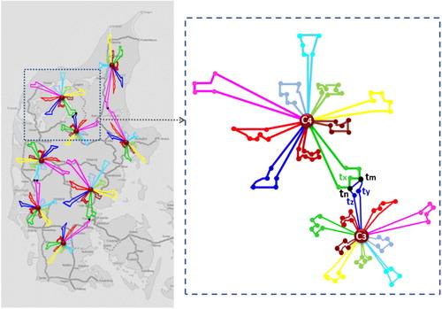
As mentioned previously, due to the nature of the tasks required to maintain a railway system using ERTMS, not all tasks can be assigned to only one person. For example, in Figure 1, assume that tasks tn and tm need to be done by two crew members. Although crew c3 and c4 are responsible for completing single tasks on their own routes, the maintenance plan should support daily collaboration of different crew members on such tasks. In this way, crew c3 and c4 should meet at the same time and location as part of their independent daily routes to complete this type of maintenance task as shown in Figure 1. In the maintenance planning problem faced in this article, we have not taken the skill set of the crew members into account.

2.2. MIP formulation

Here we present the MIP formulation of the problem. The temporal aspect is modelled by using ‘one vehicle-independent time variable t_i for the beginning of execution of a task or operation requiring more than one vehicle at a vertex i’ as in Drexl (2012). This way of modelling is the most popular variant among MIP-based approaches in the literature (Li et al., 2005; Lim et al., 2004; Dohn, Kolind, & Clausen, 2009; Cortés, Matamala, & Contardo, 2010). The synchronisation constraint is explicitly included in the model, inspired by the straightforward model presented by (Bredstrom & Ronnqvist, 2008). According to their work, if a task needs to be completed by two crew members, it will be duplicated; introducing a second virtual task located at the exact same coordinates and requiring the same service time. These pairs of tasks are included in a set called the P_sync set. If we ensure that a single crew member is not assigned both tasks within each pair of P_sync, the actual task will be completed by two different crew members.

Maintenance tasks are related to the geographic locations of the equipment to be serviced. Here we use a set $n\in N$ of geographical positions, referred to as task points. The task points are modelled as vertices of a graph $G=(N,A)$, connected through arcs $(i,j)\in A$, with a weight corresponding to the travel time $T_{i,j}$ between them. It takes D_i time to perform task i. There is also a time-window, inside which task i should be performed, with a_i denoting the earliest start time and b_i the latest finish time, where $a_i\ge 0$ and $b_i\ge a_i$. Each crew member $m\in M$ has an earliest start time o_m and a latest finish time d_m.

There are two types of decision variables: The variables $x_{i,j,m,k}\in 0,1$ which are 1 if crew m travels from task i to task j at day k, otherwise 0. The task-time variables $t_{i,k}\ge 0$ are the arrival time at task i at day k and are 0 if the task is not visited at day k. Hence the arrival time for a visit task i is defined by $\sum _{k\in K}{t}_{i,k}$.

This model can be seen as a generalisation of the classical Vehicle Routing Problem with Time Windows, extended with multiple depots and synchronisation requirements. The full model is given below in Equations (1)–(9).

The objective function (1) simply minimises the required transportation time: (1) $$\mathrm{M}\mathrm{i}\mathrm{n}\sum _{m\in M}\sum _{k\in K}\sum _{(i,j)\in A}{T}_{i,j}{x}_{i,j,m,k}$$(1)

Constraint (2) ensures that each signal maintenance task i is visited exactly once: (2) $$\sum _{m\in M}\sum _{k\in K}\sum _{j:(i,j)\in A}{x}_{i,j,m,k}=1\hspace{1em}\forall i\in A\hspace{1em}$$(2)

Constraints (3) and (4) represent the routing network. Constraint (3) ensures that each crew member m starts each day k from his depot and ends every day at his depot: (3) $$\begin{array}{c}\sum _{j:(o_m,j)\in A}{x}_{o_m,j,m,k}=\sum _{j:(j,d_m)\in A}{x}_{j,d_m,m,k}=1\hfill \\ \hspace{1em}\forall k\in K,m\in M\hfill \end{array}$$(3)

Constraint (4) is the flow constraint which ensures that if a crew member arrives at a task point that crew member also moves on to another task point: (4) $$\begin{array}{c}\sum _{j:(i,j)\in A}{x}_{i,j,m,k}-\sum _{j:(j,i)\in A}{x}_{j,i,m,k}=0\hfill \\ \hspace{1em}\forall k\in K,m\in M,i\in N\hfill \end{array}$$(4)

Constraints (5), (6) and (7) represent the scheduling constraints. Constraint (5) links the $x_{i,j,m,k}$ variables with the $t_{j,k}$ variables: (5) $$\begin{array}{c}{t}_{i,k}+(T_{i,j}+D_i)x_{i,j,m,k}\le t_{j,k}+b_i(1-x_{i,j,m,k})\hfill \\ \hspace{1em}\forall k\in K,m\in M,(i,j)\in A\hfill \end{array}$$(5)

Subtour constraints are satisfied by formulating the routing constraints in a multi-commodity formulation (constraint (4)) and having the subtour inequalities through constraint (5).

Constraint (6) ensures that each task i is visited inside the time window $[a_i,b_i]$: (6) $$\begin{array}{c}{a}_i\sum _{j:(i,j)\in A} x_{i,j,m,k}\le t_{i,k}\le b_i\sum _{j:(i,j)\in A} x_{i,j,m,k}\hfill \\ \hspace{1em}\forall k\in K,m\in M,i\in N\hfill \end{array}$$(6)

Constraint (7) ensures that all maintenance tasks are carried out during the working hours of crew person m: (7) $$a_{m,k}\le t_{i,k}\le b_{m,k}\hspace{1em}\forall k\in K,m\in M,i\in \{0,d\}$$(7)

Constraint (8) ensures that if task i and j must be visited by two crew members then they should arrive at the task at the same time on the same day: (8) $$\sum _{m\in M}{t}_{i,k}=\sum _{m\in M}{t}_{j,k}\hspace{1em}\forall k\in K,(i,j)\in P_{\mathit{\text{sync}}}$$(8)

Constraint (9) ensures that each crew member only visits one node of a given pair in the P_sync set on a given day. Using this constraint, we ensure a synchronised task will be assigned to two different crew members. (9) $$\begin{array}{c}\sum _{i2:(j2,i)\in A}{x}_{i2,i,o_m,k}+\sum _{i2:(j2,j)\in A}{x}_{i2,j,o_m,k}\le 1\hfill \\ \forall k\in K,(i,j)\in P_{\mathit{\text{sync}}},\forall m\in M\hfill \end{array}$$(9)

3. Proposed solution framework

Although a MIP solver might be able to solve the modelled problem up to a certain size, Banedanmark require feasible maintenance plans for around 1000 tasks over a month long period. We propose a stage-based framework using Constraint Programming (CP) on top of a MIP model used to allocate tasks to crew members. We divide the problem into the following stages, as illustrated in Figure 2.

Figure 2. An illustration of our proposed approach for solving the problem in a stage-based manner.

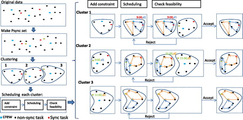
• For each task that requires synchronisation, a second virtual task with the exact same coordinates is generated.

• The tasks are split into M clusters, where M is the number of crew members. This is done by solving a clustering MIP model with a commercial MIP solver.

• The clusters are sorted according to a predefined difficulty order.

• Based on the ordered clusters, for each cluster, a Vehicle Routing Problem with Time-Windows (VRPTW) is solved as a Constraint Satisfaction Problem (CSP), considering the set of primitive constraints imposed by the synchronised tasks that have been allocated previously. These new constraints are defined on top of the VRPTW and are imposed as pre-scheduling constraints to the problem within each cluster.

• After finding a schedule for a given cluster, a look-ahead technique is used to check if this causes any infeasibility for as yet unscheduled clusters.

These steps are described in more detail in the following sub-sections.

3.1. First stage: The synchronisation set

As mentioned earlier, if a task needs to be completed by two crew members, we apply the same technique introduced by Bredstrom and Ronnqvist (2008), using a set P_sync. Assigning the actual task and its virtual pair within each pair in the P_sync set to different crew members will ensure that the synchronisation constraints are met.

3.2. Second stage: Clustering

Formally, the clustering problem requires finding a set of subsets $C=\{C_1,\dots ,C_k\}$ of N tasks, such that $N={\cup }_{i=1}^k{C}_i$ and $C_i\cap C_j=0$ for $i\ne j$. Consequently, any task in N belongs to exactly one and only one subset. It is reasonable to assume that crew members should be assigned to tasks within their geographical proximity. In addition, each crew member needs to be given approximately the same amount of work. The clustering problem is therefore formulated as follows:

Sets and parameters:

$M=$ set of crew members

$N=$ set of maintenance tasks

T_mi: travelling time between crew m and task

  $i|m\in M$ and $i\in N$

D_i: duration of task i

P_sync: set of synchronised tasks represented by

    two nodes for the same task.

Decision variables:

x_mi: 1 if task i belongs to the cluster of crew m, 0

otherwise

w: positive variable representing the maximal workload difference between two crew members in terms of total task duration.

Equations: (10) $$\mathrm{M}\mathrm{i}\mathrm{n}\hspace{1em}\lambda *\sum _{m\in M}\sum _{i\in N}{x}_{m,i}*T_{m,i}+(1-\lambda )*w$$(10) subject to: (11) $$\begin{array}{c}\sum _{i\in N}{x}_{mi}*D_i-\sum _{i\in N}{x}_{vi}*D_i\hspace{1em}\le w\hspace{1em}\hfill \\ \forall m\in M\hspace{1em}and\hspace{1em}\forall v\in M\hspace{1em}\hfill \end{array}$$(11) (12) $$\sum _{m\in M}{x}_{mi}=1\hspace{1em}\forall i\in N$$(12) (13) $$x_{m,i}+x_{m,h}\le 1\hspace{1em}\forall m\in M\hspace{1em}\mathrm{a}\mathrm{n}\mathrm{d}\hspace{1em}\forall (i,h)\in P_{\mathit{\text{sync}}}$$(13)

The objective function (10) is multi-criteria and aims to find the optimal trade-off between assigning tasks to crew members based on their proximity whilst also taking crew workload balance into account. The first term in the objective function minimises the total travel time for a crew member to their assigned tasks. The second term, w, is the greatest workload balance mismatch across different clusters as described by constraint (11). The weights assigned to the two terms of the objective function are given as λ and $1-\lambda$. Based on the results of some preliminary experimentation and consultation with the industrial partner, for the numerical results presented in this paper we use $\lambda =0.3$ and subsequently $1-\lambda =0.7$ for these weights. This gives a reasonable trade-off between workload balance and the total distance covered. Constraint (12) ensures that each task should be assigned to only one crew member and constraint (13) asserts that synchronised tasks and their virtual pairs are not assigned to the same crew member. In our experiments, the GAMS solver is used to solve this model.

3.3. Third stage: Ordering clusters

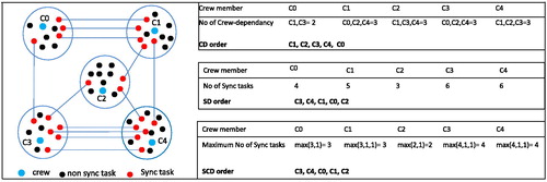
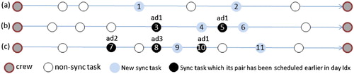
We start by ordering the clusters to be scheduled. The idea is to give priority to those clusters which are more difficult to schedule. Depending on the geographic location of a crew member, in the clustering phase some crew members more likely to be assigned synchronised tasks than others. For instance, those clusters which are surrounded by many clusters are likely to have more synchronised tasks in common with other clusters than those clusters, which are located on the edge of the region. We define three different ordering strategies according to the interdependency of the clusters based on their synchronised tasks as follows:

• Most crew dependency (CD): orders the clusters by decreasing number of neighbouring clusters with synchronised tasks.

• Largest sync dependency (SD): orders the clusters by decreasing number of synchronised tasks assigned to each crew member.

• Max sync with another crew dependency (SCD): orders the clusters in decreasing order of the number of synchronised tasks which one crew member shares with a single neighbouring crew member.

Figure 3 gives an example of the proposed ordering strategies for five crew members, showing how the clusters are ordered based on each ordering strategy. In the case of a tie, crew members with the same score are processed in an arbitrary order.

Figure 3. An example of the three ordering strategies.

3.4. Fourth stage: Routing and scheduling

After decomposing the problem into clusters and selecting a clustering ordering, the routing and scheduling problem is solved for each cluster in turn. Solving the problem in this manner is still challenging, as the presence of tasks requiring synchronisation introduces interdependencies between clusters. This interdependency can exist between routes of the current cluster and the routes of previously scheduled clusters, as well as with the potential routes of the remaining unscheduled clusters. We propose an approach that guarantees feasible solutions with respect to these synchronisation constraints, taking both situations into account. The details of this phase are explained in the following section.

4. Routing and scheduling phase

The routing and scheduling phase is run one cluster at a time, using the different cluster orderings introduced in Section 3.3. The problem for each cluster is composed of a standard Vehicle Routing Problem with Time Windows, plus a set of constraints required to manage to the potential interdependencies existing between the current cluster, previously scheduled clusters and the remaining unscheduled clusters. We define the following terms for this phase:

• Sync task: following clustering, no actual task and its pairwise virtual task are assigned to the same crew member. Therefore when scheduling each cluster, the algorithm does not differentiate whether each synchronised task of the current cluster is an actual task or a virtual task. It considers each as a sync task.

• Pair task: following from the definition of a sync task, the pairwise of each sync task is referred to as a pair task.

• Abstract day ID: is a unique identifier representing the scheduling day of a sync task. If two sync tasks have the same abstract day ID, they are scheduled to be completed on the same day. If two sync tasks in a single route have been assigned to two different abstract day IDs, the IDs can be mapped to a third abstract day ID to make sure that the tasks are completed on the same day. We use the abstract day ID concept to merge days gradually during solution construction, consequently minimising the number of working days required in the solution. This process is explained in detail in Section 4.2.4.

4.1. Route interdependency

Although the framework solves one cluster at a time, it takes the interdependencies with other clusters into consideration. To do this, a set Tuple_sync is defined with the relation $(P_{\mathit{\text{sync}}},C_{\mathit{\text{sync}}},z,at,d)$ $\in \mathit{\text{Tupl}}{e}_{\mathit{\text{sync}}}$, where C_sync is the pair of crew members assigned to pair task P_sync, z is a Boolean indicating whether a sync task or its pair have been scheduled already, at is the scheduled arrival time and d represents the scheduling day. Using $\mathit{\text{Tupl}}{e}_{\mathit{\text{sync}}}$, the framework knows whether or not a synchronised task has already been scheduled in a previous cluster. The elements in Tuple_sync change state as follows:

• Initialisation: Prior to scheduling, one relation is generated in Tuple_sync for each pair in P_sync with z initialised to false, at to 0 and d to –1, indicating that no sync task has been scheduled so far.

• During Scheduling: After scheduling a cluster, each scheduled sync task can have two different states:

  1. If the pair task has not been scheduled in a previous cluster, the related Tuple_sync should be updated by setting z to true, at to arrival time and the d to the day that the task has been scheduled.

  2. If the pair task has already been scheduled there will be no change in status. In this case, when the second sync task in a pair is scheduled, there is only the possibility that the abstract day ID will be updated.

The approach keeps track of the state of partial solutions, checking the status of the scheduled synchronised task in previous clusters, the status of the current scheduling cluster and the impact on feasibility for the remaining unscheduled clusters.

4.2. The problem as a CSP

The VRPTW problem is modelled as a CSP as below. The additional constraints added to the problem are explained in detail in the subsequent subsections.

Set: $$\begin{array}{c}N=\left\{1,\dots ,n\right\}: \text{set} \text{of} \text{tasks} \text{in} \text{all} \text{clusters} \hfill \\ M=\left\{1,\dots ,m\right\}: \text{set} \text{of} \text{all} \text{crew} \text{members} \text{or} \text{clusters}\hfill \\ K=\left\{1,\dots ,k\right\}: \text{set} \text{of} \text{days} \text{or} \text{routes}\hfill \\ N\prime =\left\{1,\dots ,n\prime \right\}: \text{set} \text{of} \text{tasks} \text{for} \text{current} \text{cluster}\hfill \\ R=K\cup \left\{0\right\}: \text{set} \text{of} \text{days},\text{including} \text{unplanned} \text{days}\hfill \\ S=\left\{\begin{array}{cc}n\prime +1\hfill & \mathrm{..}k+1\hfill \end{array}\right\}: \text{set} \text{of} \text{start} \text{visits} \hfill \\ E=\left\{\begin{array}{cc}n\prime +k+1\hfill & \mathrm{..}n\prime +2k\hfill \end{array}\right\}: \text{set} \text{of} \text{end} \text{visits} \hfill \\ V=N\prime \cup S\cup E: \text{set} \text{of} \text{all} \text{visits} \hfill \\ V^S=N\prime \cup S: \text{set} \text{of} \text{visits} \text{which} \text{have} \mathrm{a} \text{successor} \hfill \\ V^E=N\prime \cup E: \text{set} \text{of} \text{visits} \text{which} \text{have} \mathrm{a} \text{predecessor} \hfill \\ P_{\mathit{\text{sync}}}=\text{pair} \text{set} \text{of} \text{synchronised} \text{tasks} \hfill \\ C_{\mathit{\text{sync}}}=\text{pair} \text{set} \text{of} \text{crew} \text{members} \text{assigned} \text{to} \hfill \\ \text{the} \text{synchronised} \text{tasks} \hfill \\ \hfill \\ \mathit{\text{AbstractDay}}=\left\{ad|ad\in \mathcal{N}\right\} \text{set} \text{of} \text{abstract} \text{days} \hfill \\ /\text{routes} \hfill \\ \hfill \\ \mathit{\text{Tupl}}{e}_{\mathit{\text{sync}}}=\left\{\right(p,c,z,ad,at\left)\right|p\in P_{\mathit{\text{sync}}},c\in C_{\mathit{\text{sync}}},\hfill \\ z\in \left\{\mathit{\text{True}},\mathit{\text{False}}\right\},ad\in \mathit{\text{AbstractDay}},0\le at\le 12\}\hfill \end{array}$$

Parameters: $$\begin{array}{c}{c}_c\in M: \text{current} \text{crew} \text{member}/\text{cluster} \hfill \\ o_x: \text{start} \text{of} \text{the} \text{day} \mathrm{x} \text{is} \text{indexed} \text{as} \mathrm{n}\prime +\mathrm{x}\hfill \\ d_x: \text{end} \text{of} \text{the} \text{day} \mathrm{x} \text{is} \text{indexed} \text{as} \mathrm{n}\prime +\mathrm{k}+\mathrm{x}\hfill \\ a_i: \text{earliest} \text{time} \text{to} \text{start} \text{maintenance} \text{task} \mathrm{i}\hfill \\ b_i: \text{latest} \text{time} \text{to} \text{start} \text{maintenance} \text{task} \mathrm{i}\hfill \\ D_i: \text{duration} \text{of} \text{maintenance} \text{task} \mathrm{i}\hfill \\ T_{ij}: \text{travel} \text{time} \text{from} \text{task} \mathrm{i} \text{to} \text{task} \mathrm{j}\hfill \\ (\text{the} \text{task} \text{visited} \text{after} \text{task} \mathrm{i}) \hfill \end{array}$$

Decision variables: $$\begin{array}{c}nex{t}_i\in V^E\hfill \\ nex{t}_i=\{\begin{array}{c}0,\hspace{1em}i\in V^S\hfill \\ \text{index} \text{of} \text{the} \text{next} \text{visit},\hspace{1em}i\in E\hfill \end{array}\hfill \\ pre{v}_i\in V^S\hfill \\ pre{v}_i=\{\begin{array}{c}0,\hspace{1em}i\in V^E\hfill \\ \text{index} \text{of} \text{the} \text{previous} \text{visit},\hspace{1em}i\in S\hfill \end{array}\hfill \\ da{y}_i\in R: \text{index} \text{of} \text{the} \text{day}/\text{route} \text{that} \text{visits} \text{task} \mathrm{i}\hfill \\ t_i:\in {\mathcal{R}}^{+},0<t_i<12 \text{arrival} \text{time} \text{at} \text{task} \mathrm{i}\hfill \\ \mathit{\text{activ}}{e}_i:\mathit{\text{true}}\text{if} \text{task} \mathrm{i} \text{is} \text{visited} \text{other} \text{wise} \mathit{\text{false}}\hfill \end{array}$$

Objective function: $$\begin{array}{c}\sum _{i\in V^S,da{y}_i\ne 0}\hspace{1em}{T}_{i,nex{t}_i}\hfill \end{array}$$

General constraints: $$\begin{array}{c}\mathit{\text{AllDifferent}}\left(nex{t}_i,N\right)\forall i\in V^S\hfill \\ \text{ensures} \text{all} \text{nodes} \text{have} \text{only} \text{one} \text{successor}\hfill \\ \hfill \\ \mathit{\text{AllDifferent}}\left(pre{v}_i,N\right)\forall i\in V^E\hfill \\ \text{ensures} \text{all} \text{nodes} \text{have} \text{only} \text{one} \text{predecessor} \hfill \\ \hfill \\ \mathit{\text{NoCycle}}\left(nex{t}_{\ast },\mathit{\text{activ}}{e}_{\ast }\right)\hfill \\ \text{ensures} \text{no} \text{cycle} \text{exists} \text{in} \text{the} \text{routes} \hfill \end{array}$$

Consistency Constraints: $$\begin{array}{c}nex{t}_{pre{v}_i}=i\hspace{1em}\forall i\in V^S\hfill \\ pre{v}_{nex{t}_i}=i\hspace{1em}\forall i\in V^E\hfill \\ \hfill \\ da{y}_i=da{y}_{nex{t}_i}\hspace{1em}\forall i\in V^S\hfill \\ \text{task} \mathrm{i} \text{on} \text{each} \text{day}/\text{route} \text{should} \text{be} \text{the} \text{same} \text{as} \hfill \\ \text{day}/\text{route} \text{of} \text{successor} \text{next} \text{task} \mathrm{i} \hfill \\ \hfill \\ da{y}_i=da{y}_{pre{v}_i}\hspace{1em}\forall i\in V^E\hfill \\ \text{task} \mathrm{i} \text{on} \text{each} \text{day}/\text{route} \text{should} \text{be} \text{the} \text{same} \text{as}\hfill \\ \text{day}/\text{route} \text{of} \text{predecessor} \text{previous} \text{task} \mathrm{i} \hfill \end{array}$$

Accumulative time constraint: $$t_{nex{t}_i}=D_i+T_{i,nex{t}_i}\hspace{1em}\forall i\in V^S$$

Time windows constraint: $$\begin{array}{c}{t}_i\ge a_i\hspace{1em}\forall i\in V\\ t_i\le b_i\hspace{1em}\forall i\in V\end{array}$$

4.2.1. Adding constraints

When a cluster is being scheduled, the algorithm checks whether the pair task of each sync task in that cluster has already been scheduled in a previous cluster. This can be identified by checking the flag z in Tuple_sync to see if it is true or false. If z is false, indicating that the sync task has not been scheduled yet, no constraints are imposed on the planning day for that task. In the case that z is true, three constraints are imposed on the cluster schedule due to the existing sync task: same time schedule, same route constraint and different route constraint. The first constraint implies an explicit synchronisation constraint, similar to in the original MIP model. The other two add restrictions to the cluster schedule according to the status of the other sync tasks in the same cluster.

• Same time schedule: This constraint explicitly forces each sync task in the currently selected cluster to be scheduled at the same arrival time as their pair task, if the pair task has already been scheduled within another cluster. The arrival time can be retrieved from the record in Tuple_sync updated by the pair task. $$\begin{array}{c}{t}_i=atif\exists (p,c,z,ad,at)\in \mathit{\text{Tupl}}{e}_{\mathit{\text{sync}}}:\\ i\in p,z=\mathit{\text{True}}\end{array}$$

• Same route constraint: If there are one or more sync tasks in the current cluster where their pair tasks have already been scheduled on the same day (although not necessarily with the same crew member), all of these sync tasks should be scheduled on the same day within the current cluster. This can be tracked by looking at the Tuple_sync records which belong to the sync tasks in the current cluster (using P_sync), where the z flag is true and have the same abstract day ID. Accordingly, a constraint is added to force the current sync task to be scheduled on the same day as the other sync tasks with the same abstract day ID in the current cluster. $$\begin{array}{c}da{y}_i=adif\exists \mathit{\text{Tupl}}{e}_{\mathit{\text{sync}}}(p,c,z,ad,at)\\ \in \mathit{\text{Tupl}}{e}_{\mathit{\text{sync}}}:i\in p_{\mathit{\text{sync}}},z=\mathit{\text{True}}\end{array}$$

• Different route constraint: If there is more than one sync task in the current cluster with a pair task scheduled with different crew members on different days (i.e., they have different abstract day IDs), we can check whether these can be reassigned to the same day. If the plans of the previous crew members do not conflict with one another, the abstract day IDs could be updated to a new unique ID; consequently providing an opportunity to schedule their pair tasks in the current cluster on the same day. This does not force any changes to the routes of previously scheduled crew members.

• If any of the sync tasks cannot be scheduled on the same day due to a conflict with the pair tasks of previously scheduled clusters, a constraint is added, ensuring that these two sync tasks are not scheduled in the same day. On this basis, we define a set called CONF_i for each sync task i in the current cluster, which returns all pairs of schedules for two different crew members (m₁, m₂) from previous clusters where there is the possibility of a conflict existing between their daily time schedules (ad₁, ad₂). $$\forall i\in P_{\mathit{\text{sync}}}andi\in n\prime :$$ $$CON{F}_i=\left\{\left(m_1,a{d}_1,m_2,a{d}_2\right)\right|$$ $$\forall \mathit{\text{tuple}}1,\mathit{\text{tuple}}2\in \mathit{\text{Tupl}}{e}_{\mathit{\text{sync}}},$$ $$\mathit{\text{tuple}}1=\left(P_1,C_1,z_1,a{d}_1,a{t}_1\right),$$ $$\mathit{\text{tuple}}2=\left(P_2,C_2,z_2,a{d}_2,a{t}_2\right),$$ $$(i\in P_1)and(j\in n\prime )\in P_2),$$ $$(c\_c\in C_1)and(c\_c\in C_2),$$ $$z_1=z_2=\mathit{\text{true}},$$ $$a{d}_1\ne a{d}_2,$$ $$\exists m1\in C_{1}andm1\ne c\_c,$$ $$\exists m2\in C_{2}andm2\ne c\_c,$$ $$m1\ne m2\}$$

After this, for each member of CONF_i, for example $(m_1,a{d}_1,m_2,a{d}_2)$, a check is made for conflicts in the daily plan of crew member m1 in d1 with the daily plan of crew member m₂, including possible plans of other crew members on d₁ or d₂. This can be checked in Tuple_Sync. In the case a conflict is found, the following Global Constraint (Beldiceanu, Carlsson, & Rampon, 2005) is added to the model: $$\mathit{\text{All}}\mathit{\text{Different}}(da{y}_{d1},da{y}_{d2})$$

4.2.2. Solving the routing and scheduling problem

Solving this problem corresponds to solving a single depot vehicle routing problem with time windows (VRPTW) with the constraints imposed as defined above. To solve the VRPTW, the Routing Library (RL) is used, embedded as a layer on top of the CP solver in Google OR-Tools (Google, 2012). OR-Tools provide a number of methods to generate the first solution for CSPs. As preliminary work, we tested the Saving, Sweep, Best Insertion and Path Cheapest Arc heuristics on a small data instance with 100 tasks located exactly on rail tracks. Of these four heuristics, only Path Cheapest Arc could generate a solution within a time limit of 30 minutes and therefore used in our experimentation. Path Cheapest Arc is described as follows: ‘The heuristic starts searching from a depot, connects it to the node which produces the cheapest route segment, then extends the route by iterating on the last node added to the route’ (Google, 2012).

4.2.3. Feasibility check

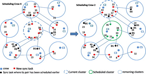
After finding a schedule for a given cluster, a look-ahead technique is used check if this causes any infeasibility for the remaining clusters to be scheduled. In the case that a synchronised task has been assigned and this is the first crew member to be allocated that task, their schedule is imposed on the crew member who is responsible for the related pair task in a subsequent cluster. This requires checking whether the second crew member is available at the scheduled time.

An example is given in Figure 4. Crew member 4 (c4) is the first to be scheduled. As tasks 36 and 38 are fixed to the same route (day 1), consequently the pair tasks 15 (for crew member 2) and 17 (for crew member 1) are fixed to day 1 as well. After finding a schedule for crew member 2 we should check whether this is feasible for tasks 14, 15 and 17. In this example, since tasks 35, 37 and 15 are assigned to the same route and since task 15 is already assigned to day 1, we have then imposed that tasks 14, 16 and 17 should be performed on day 1 as well. Here we should check whether crew member 1 will be able to complete tasks 14, 16 and 17 according to their fixed arrival times. If not, we reject the schedule for crew member 2 and randomly generate a new schedule (using a different seed in Google OR-Tools) and check for feasibility again. Likewise we should check the feasibility of the schedule for task 23 for crew member 0 and task 42 for crew member 7. This process continues until a feasible solution is found, then the schedule for crew member 2 will be accepted and the framework will move on to the next cluster.

Figure 4. This figure illustrates the order in which the entire scheduling problem is solved for several crew members (depots) over several days (routes), with special focus on the synchronised tasks which make the problem non-decomposable.

4.2.4. Updating and merging abstract day IDs

After scheduling a cluster, the result is a multi-day plan consisting of several separate routes, each starting from a crew members home location, visiting several tasks and ending back at the home location. The framework assigns the same abstract day ID to all of the synchronised tasks scheduled within the same route. After updating Tuple_sync, the framework proceeds to the next cluster, repeating this process until all clusters are scheduled.

To demonstrate the process of assigning unique IDs to synchronised tasks, we give an example for an instance with 24 maintenance tasks, eight crew members and 12 tasks requiring service from two crew members simultaneously. We introduce $U=\{0,\dots ,43\}$ nodes where $O_m=\{0,\dots ,7\}$ are crew members. The actual maintenance tasks are represented by nodes $\{8,\dots ,31\}$. 12 maintenance tasks are randomly chosen to be sync nodes: {8, 9, 13, 14, 15, 16, 17, 19, 20, 21, 22, 23}. Finally, nodes $\{32,\mathrm{..},43\}$ are created as virtual pair tasks for the sync tasks. Table 1 shows how Tuple_sync is updated at each step of crew scheduling in this situation. Synchronised tasks are given in $P\_\mathit{\text{sync}}$. For each task in these pairs, the corresponding crew is given in the tuple C_sync. z is a Boolean indicating whether the sync pair has been fixed (T) or not (F). The scheduled day is denoted as d and finally at is the arrival time at the sync node.

Table 1. This table illustrates the update process for Tuple_sync as the schedule for each cluster is decided.

Initialisation					Crew 4					Crew 2
$P\_\mathit{\text{sync}}$	$C\_\mathit{\text{sync}}$	z	d	at	$P\_\mathit{\text{sync}}$	$C\_\mathit{\text{sync}}$	z	d	at	$P\_\mathit{\text{sync}}$	$C\_\mathit{\text{sync}}$	z	d	at
(8,32)	(3,5)	F	0	0	(8,32)	(3,5)	F	0	0	(8,32)	(3,5)	F	0	0
(9,33)	(3,4)	F	0	0	(13,34)	(3,6)	F	0	0	(13,34)	(3,6)	F	0	0
(13,34)	(3,6)	F	0	0	(14,35)	(1,2)	F	0	0	(19,39)	(0,6)	F	0	0
(14,35)	(1,2)	F	0	0	(16,37)	(1,2)	F	0	0	(9,33)	(3,4)	T	1	370
(15,36)	(2,4)	F	0	0	(19,39)	(0,6)	F	0	0	(17,38)	(1,4)	T	1	281
(16,37)	(1,2)	F	0	0	(22,42)	(2,7)	F	0	0	(20,40)	(4,6)	T	1	97
(17,38)	(1,4)	F	0	0	(23,43)	(0,2)	F	0	0	(21,41)	(4,6)	T	1	24
(19,39)	(0,6)	F	0	0	(9,33)	(3,4)	T	1	370	(14,35)	(1,2)	T	1	446
(20,40)	(4,6)	F	0	0	(15,36)	(2,4)	T	1	194	(15,36)	(2,4)	T	1	194
(21,41)	(4,6)	F	0	0	(17,38)	(1,4)	T	1	281	(16,37)	(1,2)	T	1	369
(22,42)	(2,7)	F	0	0	(20,40)	(4,6)	T	1	97	(22,42)	(2,7)	T	2	63
(23,43)	(0,2)	F	0	0	(21,41)	(4,6)	T	1	24	(23,43)	(0,2)	T	1	274
Crew 6					Crew 1					Crew 3
(8,32)	(3,5)	F	0	0	(8,32)	(3,5)	F	0	0	(14,35)	(1,2)	T	1	446
(9,33)	(3,4)	T	1	370	(9,33)	(3,4)	T	1	370	(15,36)	(2,4)	T	1	194
(14,35)	(1,2)	T	1	446	(13,34)	(3,6)	T	3	231	(16,37)	(1,2)	T	1	369
(15,36)	(2,4)	T	1	194	(15,36)	(2,4)	T	1	194	(17,38)	(1,4)	T	1	281
(16,37)	(1,2)	T	1	369	(19,39)	(0,6)	T	3	96	(19,39)	(0,6)	T	3	96
(17,38)	(1,4)	T	1	281	(20,40)	(4,6)	T	1	97	(20,40)	(4,6)	T	1	97
(22,42)	(2,7)	T	2	63	(21,41)	(4,6)	T	1	24	(21,41)	(4,6)	T	1	24
(23,43)	(0,2)	T	1	274	(22,42)	(2,7)	T	2	63	(22,42)	(2,7)	T	2	63
(13,34)	(3,6)	T	3	231	(23,43)	(0,2)	T	1	274	(23,43)	(0,2)	T	1	274
(19,39)	(0,6)	T	3	96	(14,35)	(1,2)	T	1	446	(8,32)	(3,5)	T	4	86
(20,40)	(4,6)	T	1	97	(16,37)	(1,2)	T	1	369	(9,33)	(3,4)	T	1	370
(21,41)	(4,6)	T	1	24	(17,38)	(1,4)	T	1	281	(13,34)	(3,6)	T	3	231
Crew 0					Crew 7					Crew 5
(8,32)	(3,5)	T	4	86	(8,32)	(3,5)	T	4	86	(9,33)	(3,4)	T	1	370
(9,33)	(3,4)	T	1	370	(9,33)	(3,4)	T	1	370	(13,34)	(3,6)	T	3	231
(13,34)	(3,6)	T	3	231	(13,34)	(3,6)	T	3	231	(14,35)	(1,2)	T	1	446
(14,35)	(1,2)	T	1	446	(14,35)	(1,2)	T	1	446	(15,36)	(2,4)	T	1	194
(15,36)	(2,4)	T	1	194	(15,36)	(2,4)	T	1	194	(16,37)	(1,2)	T	1	369
(16,37)	(1,2)	T	1	369	(16,37)	(1,2)	T	1	369	(17,38)	(1,4)	T	1	281
(17,38)	(1,4)	T	1	281	(17,38)	(1,4)	T	1	281	(19,39)	(0,6)	T	3	96
(20,40)	(4,6)	T	1	97	(19,39)	(0,6)	T	3	96	(20,40)	(4,6)	T	1	97
(21,41)	(4,6)	T	1	24	(20,40)	(4,6)	T	1	97	(21,41)	(4,6)	T	1	24
(22,42)	(2,7)	T	2	63	(21,41)	(4,6)	T	1	24	(22,42)	(2,7)	T	2	63
(19,39)	(0,6)	T	3	96	(23,43)	(0,2)	T	1	274	(23,43)	(0,2)	T	1	274
(23,43)	(0,2)	T	1	274	(22,42)	(2,7)	T	2	63	(8,32)	(3,5)	T	4	86

The abstract day ID distinguishes between each planning day of a crew member’s schedule, enabling us to identify the dependency between crew plans assigned the same abstract day ID for synchronised tasks. After scheduling the current cluster, the algorithm may encounter three different situations for each route (daily plan) as shown in Figure 5. Situation (a) occurs when the route contains only synchronised tasks where their pair tasks have not already been scheduled (task 1 and 2). In this case, the synchronised tasks are assigned an abstract day ID and the d value and z flag are updated to true.

Figure 5. Three possible situations of the generated routes in one cluster after the scheduling step.

The second situation happens when the route has one or more synchronised tasks with pair tasks that have already been scheduled on the same day (i.e., they have the same abstract day ID and the z flag is true). For instance in Figure 5b, the pairwise tasks with IDs 3 and 5 have already been scheduled in day 1 as shown. In this case, the algorithm only updates the records of other existing synchronised tasks in the route where their pair tasks have not already been scheduled (tasks with ID 4 and 6), to the same abstract day ID of the others (ad1).

As explained earlier regarding the different route constraint, the algorithm checks the feasibility of the scheduling on the same day of the sync tasks in the current cluster with their pair task, to see if they have already been scheduled on different days for different crew. In the case of infeasibility due to a conflict in crew plans, the algorithm adds the different route constraint. In the case of feasibility, the schedule of the current cluster could result in a route having synchronised tasks with different abstract IDs, e.g. route (c) has sync tasks 7, 8 and 10 scheduled in day IDs 2, 3 and 1 respectively. In this case, the algorithm gives a new unique abstract ID to all of the synchronised tasks scheduled in the current route including the new sync tasks (those tasks whose pairs have not been scheduled earlier in previous clusters) as well. For instance, in route (c), the corresponding records of tasks 7, 8, 10, 9 and 11 in Tuple_sync, as well as all sync tasks scheduled in days 2 or 3 or 1 are updated to a new unique ID. Moreover, the algorithm should do one more extra step in this situation by updating all of the day IDs of any other pair tasks in the whole Tuple_sync whose IDs are either 2, 3 or 1.

It should be noted that updating the abstract day ID does not make any changes to the routes, only the actual day that each route is completed by crew members. As every unique abstract day ID is representative of a different day, this is an effective approach to reduce the total number of working days in the solution. However, as the generated plans use abstract day IDs, a mapping to actual day numbers is required. For example, a generated plan with a total of three working days could have abstract day IDs 4, 9 and 6 which ultimately need to be mapped to the actual day IDs 2, 3 and 1, accordingly.

5. Experimental results

In this section we report the results of experiments using the stage-based solution approach described in Sections 3 and 4 for set of test cases covering a number of scenarios. All experiments were run on a Core (TM) i7-4600U CPU 2.10 GHz processor, with 8.00 GB RAM.

5.1. Test case description

Each test case consists of a set of geographical points (tasks), demand (number of crew members required to perform a task) and time window constraints for attending a task. For each data instance, 10% of tasks are syncronised tasks, requiring two crew members to be completed. According to Banedanmark, all inspection tasks for signalling components take less than 2 hours. This is in line with the description of (Liden, 2014), where all railway maintenance activities were listed with the required completion time. There, the time required to complete a single signalling task is reported to be up to 1 hour, with planning typically required to be completed 1 month in advance. Accordingly, we define the duration of each task as 1 hour in our model.

All tasks are located within the Danish peninsular of Jutland. The coordinates representing the geographical location of the tasks have been randomly generated by utilizing the Google Maps API, using three different data generation approaches:

• Exact (E). Tasks are all located on the rail tracks of the maintenance area.

• Mixed (M). Tasks are located randomly on or off-track.

• Random (R). Tasks are scattered around the whole area randomly.

For each of these approaches, test cases containing 100, 500 and 1000 tasks are generated, resulting in a total of nine problem instances. The maintenance team in each case consists of eight crew members. The Haversine formula (Van Brummelen, 2013), often used in navigation, is used to calculate the distance between tasks. This formula provides the great-circle distance (i.e., shortest distance over the earth’s surface) between two pairs of latitudes and longitudes. Figure 6 provides visualisations for each of the test cases.

Figure 6. Geographical visualisation of the dataset.

5.2. Comparison with a commercial MIP solver

As preliminary work, in order to validate the need for the proposed CSP approach, we compared our framework to a commercial MIP solver, modelling the PSMCSP as a mixed integer programming model in GAMS. The MIP solver used is CPLEX 12.4 given a time limit of one hour, with default parameter settings and the optcr parameter set to 0.001. We tested the problem on five small data instances, with eight crew members, with a set of mixed tasks placed randomly on or off-track. The datasets are named M24-0, M24-3, M24-5, M48-0 and M48-5 corresponding to instances with 24 or 48 tasks of which 0, 3 or 5 are synchronised tasks.

Table 2 compares the travelling time values and relative gaps of the solutions generated using the stage-based CP framework, and the best solution obtained by a commercial MIP solver. The optimality gap shown using MIP solver is the gap obtained within the 1 hour time limit. As mentioned earlier, since clusters are scheduled sequentially in our framework, we present the travelling distance (Cost), the lower bound, and the optimality gap per generated cluster. Total travel time within the solution and CPU time taken to construct the solution are also given.

Table 2. Comparison between the proposed constructive framework and a MIP solver on small data instances.

Dataset	Proposed constructive framework						MIP solver (time limit: 1 hour)
	Depot	Distance	LB	Gap	Travel Time(h)	CPU Time(ms)	Travel Time(h)	LB	Relative Gap
	7	138564	129006	6.90%	1.75	102.01
	6	41366	41366	0%	0.53	2.00
	5	139979	94336	32.61%	1.73	17.00
M24-0	4	71975	58228	19.10%	0.92	3.00
	3	87062	83988	3.53%	1.08	4.00
	2	107530	79996	25.61%	1.35	8.00
	1	98739	66428	32.72%	1.22	18.00
	0	191944	121724	36.58%	2.42	18.00
	Total	877159	675072		11.00	172.01	9.58	9.57	0.09%
	4	113885	103546	9.08%	1.43	34.00
	6	41366	41366	0%	0.53	4.00
	5	139979	94336	32.61%	1.73	9.00
M24-3	2	181692	151022	16.88%	2.27	36.00
	1	233157	201877	13.42%	2.90	36.00
	7	180212	174921	2.94%	2.27	26.00
	3	87062	83988	3.53%	1.08	3.00
	0	163158	128946	20.97%	2.05	4.00
	Total	1140511	980002		14.27	152.01	11.16	10.45	6.35%
	4	113885	103546	9.08%	1.43	38.00
	6	41366	41366	0%	0.53	6.00
	5	139979	94336	32.61%	1.73	15.00
M24-5	2	181692	151022	16.88%	2.27	24.00
	1	280719	96888	65.49%	3.50	61.00
	7	180212	174921	2.94%	2.27	26.00
	3	87062	83988	3.53%	1.08	3.00
	0	163158	128946	20.97%	2.05	5.00
	Total	1188073	875013		14.87	178.01	11.67	9.86	15.52%
	7	217760	170095	21.89%	2.73	88.01
	6	102548	80198	21.79%	1.25	52.00
	5	212079	146610	30.87%	2.67	95.01
M48-0	4	97942	64512	34.13%	1.23	14.00
	3	138678	112244	19.06%	1.73	17.00
	2	212828	178022	16.35%	2.65	125.01
	1	133370	74666	44.02%	1.67	13.00
	0	146874	116542	20.65%	1.83	16.00
	Total	1262079	942889		15.77	420.02	29.28	9.66	67.01%
	4	107421	86978	19.03%	1.33	46.00
	6	172976	120162	30.53%	2.13	93.01
	2	280133	246754	11.92%	3.52	457.03
M48-5	7	217760	170095	21.89%	2.73	53.00
	5	212079	146610	30.87%	2.67	81.00
	3	138678	112244	19.06%	1.73	13.00
	1	133370	74666	44.02%	1.67	12.00
	0	146874	116542	20.65%	1.83	14.00
	Total	1409291	1074051		17.62	769.04	No integer solution found

As shown, for the data instance M24-0, the MIP solver can generate the optimal solution with travelling time 9.58 hours, while our approach generates a first feasible solution with travelling time 11.00 hours. For instances M24-3 and M24-5, the MIP solver generates solution with objective function value and optimality gap of 11.16, 6.35%, and 11.67, 15.52%, respectively. For these instances, our framework generates initial solutions with an objective value of function of 14.27 and 14.87 hours.

When the size of the instance is increased to 48 tasks, the limitations of using a MIP solver for this problem become apparent. The results for data instance M48-0 show that our framework is able to generate a better solution (15.77) in less than half a second (420.02 ms) than the MIP solver is able to after an hour (29.28).

Finally, for data instance M48-5 the strengths of the framework are particularly notable. For this dataset, containing 48 tasks of which 5 are synchronised, the MIP solver is not able to produce a solution within the time limit. However, the proposed CP framework generates a feasible solution for the same dataset within less than a second (769.04 ms).

5.3. Main results

For the nine problem instances introduced in Section 5.1, the proposed framework is run once for each of the three different cluster orderings from Section 3.3: CD, SD and SCD. The results are compared in Table 3. The values compared in the columns of this table include total driving distance for all crew members (Distance), the minimum number of working days (Days), total travel time in hours (Travel Time), and CPU time in seconds.

Table 3. Results of solving the nine datasets based on three different cluster ordering methods.

Order: Most crew dependency degree first (CD)
Dataset	Distance (km)	Days	Travel time (h)	CPU time (s)
E100	3385.69	3	42.22	0.58
E500	10767.27	16	134.43	40.60
E1000	19441.38	26	242.13	1104.94
M100	3473.82	4	43.42	1.23
M500	9906.69	15	123.78	34.28
M1000	16590.22	24	206.83	89.59
R100	3166.45	4	39.63	0.13
R500	9447.19	12	118.05	3.46
R1000	15648.66	24	195.58	30.13
Order: Largest sync degree first (SD)
E100	3147.79	3	39.22	0.03
E500	10633.49	13	132.58	8.49
E1000	18847.46	23	234.53	114.11
M100	4104.92	4	51.27	0.10
M500	9917.30	15	123.93	3.87
M1000	16786.57	24	209.42	65.31
R100	3064.10	4	38.32	0.11
R500	10109.71	14	126.30	2.47
R1000	16156.64	27	201.82	32.32
Order: Max sync to one crew degree first (SCD)
E100	3441.53	4	42.88	0.02
E500	10633.49	13	132.58	8.46
E1000	19526.82	27	243.27	125.63
M100	3920.73	4	48.97	0.08
M500	10089.00	15	126.10	4.04
M1000	18450.14	26	230.10	104.55
R100	3166.45	4	39.63	0.09
R500	9502.10	13	118.73	2.30
R1000	16165.13	26	202.03	35.10

There are a number of interesting observations that we can make based on these results. First, note that the overall computational time is very low, ranging from a few seconds for the smallest instances, to a few minutes for the biggest instances (with 1000 tasks). This is unusual for an NP-hard problem, especially when the original MIP model is not able to solve the instances with more than around 24 tasks as observed above. Using our stage-based method we are not only able to find a feasible initial solution for monthly plans with 1000 tasks, but we are also able to find different feasible solutions. This can prove useful in future work for improving upon initial feasible solutions.

The second observation is that the order in which we do the clustering has some impact on the performance of the algorithm. This is due to the feasibility checks performed at each step. For the ordering based on crew dependency on other crew members (CD), there is a case (E1000) where the algorithm has to run for 18 minutes to find a solution. When we use the ordering based on the largest sync task dependencies of each crew member (SD), however, the problem is solved within a couple of minutes. The third ordering method (SCD) produces poorer quality results in general compared to the other two ordering methods.

A third observation is that by looking at total travelling distance and minimum number of scheduling days, we notice that the solutions generated by using CD ordering outperform the obtained results using the SD order for the data sets M100, M500, M1000 and R100, R500, R1000 whereas the opposite is the case for the data sets E100, E500, E1000 – that is, the cases where all signals are on the rail tracks. This is likely due to the fact that when using the SD order for clustering, many sync tasks are fixed to the same day early on in the process. This is reasonable because there is less travelling distance between the tasks located exactly on the tracks. Since a seemingly good structure is fixed in the earlier phases of the scheduling process, it is easier to find good quality sub-solutions in later clusters where there is less dependency on the sync tasks. In contrast, for the other data sets, where the sync tasks are geographically scattered, CD generates better results, distributing the sync tasks more widely over different routes in the early stages of the algorithm.

5.4. Individual cluster results

To give an idea of how the tasks are scheduled over the individual clusters, we will show the detailed results generated by using the SD ordering for E100, E500 and E1000, since these are the instances which most resemble the real world problem. Table 4 shows the results within each clusters for these datasets. Results are given for each crew member, providing the total driving distance, number of tasks assigned, number of working days, travelling time, and CPU time required to calculate the results. The totals across all clusters for that instance are also given.

Table 4. The results for individual clusters based on SD ordering for the on track data instances.

E100
CrewId	Distance (km)	Task duration (h)	Days	Travel time (h)	CPU time (s)
3	426.00	14.00	3	5.32	0.002
6	446.07	14.00	3	5.57	0.010
0	395.92	14.00	3	4.93	0.001
2	411.95	13.00	3	5.15	0.002
5	453.82	14.00	3	5.63	0.004
4	276.98	14.00	3	3.43	0.000
7	305.75	13.00	3	3.82	0.010
1	431.30	14.00	3	5.37	0.000
Total	3147.79	110.00	3	39.22	0.029
MAD	51.05	0.38	0.00	0.64	0.003
MAD / Mean	0.13	0.03	0.00	0.13	0.905
E500
6	1736.87	69.00	11	21.72	0.03
3	2024.87	69.00	13	25.22	1.43
4	1065.45	69.00	12	13.28	2.67
0	909.40	68.00	11	11.38	0.04
1	1224.66	69.00	10	15.27	0.03
7	1079.47	69.00	11	13.40	2.45
5	1487.51	69.00	12	18.50	1.13
2	1105.26	68.00	11	13.82	0.72
Total	10633.49	550.00	13	132.58	8.49
MAD	315.42	0.38	0.72	3.93	0.86
MAD / Mean	0.24	0.01	0.06	0.24	0.81
E1000
6	3017.67	137.00	21	37.55	0.12
3	3777.11	137.00	23	47.05	19.63
5	2694.98	137.00	23	33.55	21.29
0	1593.51	138.00	21	19.77	22.16
1	2555.68	138.00	22	31.88	34.94
4	1661.89	138.00	22	20.63	8.67
2	1731.61	138.00	22	21.57	7.26
7	1815.02	137.00	21	22.53	0.05
Total	18847.46	1100.00	23	234.53	114.11
MAD	655.42	0.50	0.66	8.19	10.24
MAD / Mean	0.28	0.00	0.03	0.28	0.72

The Mean Absolute Deviation (MAD) is calculated for each value across the eight clusters. MAD gives a measure of dispersion across different clusters. The lower the MAD, the more balanced a solution is. To make the MAD of one measurement comparable with the MAD of other measurements, the MAD/Mean ratio is calculated, rescaling the MAD by dividing it by the Mean.

Looking at the MAD values, we notice a relatively modest level of deviation from the average in terms of the distance covered by each crew member. Likewise, the deviation of task durations is less than 1 hour and the deviation of the number of scheduling days is less than 1 day for all data sets.

By ranking the MAD/Mean value for all measurements in each data set and comparing the ranking in all data sets, we can see that the clusters are more homogenized according to the following order: task duration 0.03, 0.01, 0.00, days 0.00, 0.06, 0.03, total distance and total travelling time 0.13, 0.24, 0.28 (as they are proportional), and finally CPU time 0.905, 0.81, 0.72 for dataset E100, E500 and E1000, respectively. The only exception is the number of scheduling days for E100 with MAD/Mean 0.00 which has a better rank regarding time duration with MAD/Mean value 0.03.

5.5. Optimality gap

The vehicle Routing Library (RL) of Google-OR tools can compute a lower bound on the objective function. This is done by creating a bipartite graph on the routing problem and accordingly solving a Linear Assignment Problem (Google, 2012). Specifically in our problem, since clusters are scheduled sequentially and not as a whole problem, we could only calculate the lower bound of each individual cluster using the RL. We present the travelling time (T_T), the total distance (D), the lower bound (LB), and the optimality gap(Gap) per generated cluster, using all three ordering strategies on the data instances with 100 tasks in Table 5. This gives us an idea of how similar the solutions are from cluster to cluster in terms of quality.

Table 5. Solution quality statistics per clusters for problem instances with 100 tasks.

Order: CD
E100				M100				R100
T_T(h)	D(km)	LB	Gap	T_T(h)	D(km)	LB	Gap	T_T(h)	D(km)	LB	Gap
5.83	466.7	245.456	47.41%	3.90	311.752	207.261	33.52%	4.60	368.028	168.75	54.15%
5.58	446.072	184.48	58.64%	4.51	360.487	116.482	67.69%	4.65	372.213	201.792	45.79%
4.95	395.92	203.722	48.54%	6.61	528.56	159.618	69.80%	5.53	442.19	266.512	39.73%
5.15	411.946	155.314	62.30%	6.67	533.994	316.038	40.82%	5.81	464.642	176.094	62.10%
4.27	341.709	99.686	70.83%	6.47	517.954	129.98	74.91%	3.76	300.77	145.952	51.47%
3.82	305.749	74.01	75.79%	3.03	242.36	72.744	69.99%	5.62	449.99	245.087	45.54%
5.39	431.299	78.097	81.89%	7.29	582.986	268.521	53.94%	4.46	357.006	185.79	47.96%
7.33	586.299	215.34	63.27%	4.95	395.728	154.066	61.07%	5.15	411.608	167.148	59.39%
MAD			9.44%				12.16%				6.01%
MAD/Mean			0.15				0.21				0.12
Order: SD
5.33	426.002	245.456	42.38%	5.35	427.89	207.261	51.56%	3.92	313.751	176.094	43.87%
5.58	446.072	184.48	58.64%	4.58	366.541	72.744	80.15%	5.76	460.405	266.512	42.11%
4.95	395.92	203.722	48.54%	7.54	603.276	316.038	47.61%	5.04	402.865	201.792	49.91%
5.15	411.946	155.314	62.30%	6.66	532.762	154.066	71.08%	4.60	368.028	168.75	54.15%
5.67	453.82	215.34	52.55%	8.91	713.029	159.618	77.61%	5.14	411.286	167.148	59.36%
3.46	276.978	99.686	64.01%	4.51	360.482	116.482	67.69%	4.46	357.006	185.79	47.96%
3.82	305.749	74.01	75.79%	6.47	517.954	129.98	74.91%	3.76	300.77	145.952	51.47%
5.39	431.299	78.097	81.89%	7.29	582.986	268.521	53.94%	5.62	449.99	245.087	45.54%
MAD			10.24%				10.90%				4.43%
MAD/Mean			0.17				0.17				0.09
Order: SCD
5.74	459.433	215.34	53.13%	2.87	229.601	72.744	68.32%	4.65	372.213	201.792	45.79%
6.82	545.98	184.48	66.21%	7.54	603.276	316.038	47.61%	5.53	442.19	266.512	39.73%
6.83	546.079	245.456	55.05%	5.60	447.73	154.066	65.59%	4.60	368.028	168.75	54.15%
5.37	429.279	78.097	81.81%	5.82	465.673	207.261	55.49%	5.15	411.608	167.148	59.39%
4.95	395.92	203.722	48.54%	8.91	713.029	159.618	77.61%	5.81	464.642	176.094	62.10%
5.60	448.293	155.314	65.35%	4.51	360.482	116.482	67.69%	4.46	357.006	185.79	47.96%
3.88	310.793	99.686	67.93%	6.47	517.954	129.98	74.91%	3.76	300.77	145.952	51.47%
3.82	305.749	74.01	75.79%	7.29	582.986	268.521	53.94%	5.62	449.99	245.087	45.54%
MAD			8.99%				8.66%				6.01%
MAD/Mean			0.14				0.14				0.12

MAD values are given for the obtained gaps across all clusters for each data instance. Examining the MAD values, we can see that the gaps range between 4.43% for data instance R100 using SD ordering and 12.16% for data instance M100 using CD ordering, in the best and the worst case respectively. As this range is relatively small, it indicates that solutions with similar quality per cluster are found for each data instance. Considering the MAD/Mean value specifically in each ordering, CD generates a more diverse solutions in terms of quality per cluster with values of 0.15, 0.21, and 0.12 on E100, M100 and R100, respectively. This is not the case for both SCD and SD, which generate solutions with the same deviation for E100 and M100 data instances (0.17 by SD and 0.14 by SCD).

6. Conclusion

In this study, we have proposed a mathematical model to address the Preventive Signalling Maintenance Crew Scheduling problem for the Danish railway system using ERTMS. The proposed model is a generalisation of a vehicle routing and scheduling model with synchronisation constraints, adding multiple depots and a time horizon of up to a month. A stage-based solution approach is proposed to solve the problem for realistic problem instances. The first step is a MIP-based clustering approach to distribute tasks among the crew members. The second step is a Constraint Programming based approach to generate an initial solution by scheduling clusters according to a specific order. We defined three different ordering strategies, based on the dependencies between clusters arising due to the tasks requiring synchronisation.

Experimental results indicate that the proposed approach can easily schedule up to 1000 tasks for a monthly plan for eight crew members. Comparing the total traveling distance and the number of days for each of the three orderings shows that SD ordering generates the best result for data sets on the track, while CD ordering outperforms SD ordering, with a lower total traveling distance and a smaller minimum number of days, for random problem instances. Scheduling clusters by SCD ordering gives the worst results. To analyze the impact of the generated clusters prior to the scheduling phase, we calculated the Mean Absolute Deviation (MAD) value of the measurements over each cluster and the results showed promising distribution of the measurements among all crew members.

We see a number of directions for improving the initial solutions which future research will focus on. One possibility is to use metaheuristics to construct or improve solutions to this problem. Another is the improvement of solutions by a hyper-heuristic framework, an idea which has been successfully employed for a similar problem previously (Pour, Drake, & Burke, 2018). This is suggested since the current search space of the possible solutions is limited to each ordering strategy. This can be improved by the idea of employing a combination of orderings to explore a larger area of the search space. A learning mechanism can lead the framework to select an appropriate cluster to schedule at each decision point. Finally, matheuristics, which combine metaheuristic and exact methods, could potentially improve the solutions of this paper. This is a particularly interesting option since here we have presented a framework that generates several different initial solutions to use as a starting point.

References

- Abed, S. K. (2010). European rail traffic management system – an overview. In 2010 1st International Conference on Energy, Power and Control (EPC-IQ), IEEE (pp. 173–180).
- Amraoui, A. E., & Mesghouni, K. (2014). Colored petri net model for discrete system communication management on the European rail traffic management system (ERTMS) level 2. In Proceedings of the 2014 UKSim-AMSS 16th International Conference on Computer Modelling and Simulation, UKSIM 2014, IEEE Computer Society (pp. 248–253).
- Banedanmark. (2009). The signalling programme - a total renewal of the danish signalling infrastructure (Technical report). Trafikministeriet.
- Banedanmark. (2016). Organisation, http://uk.bane.dk/visArtikelBred_eng.asp?artikelID=1446. [Online; accessed 12-December-2016].
- Barger, P., Schon, W., & Bouali, M. (2014). A study of railway ERTMS safety with colored petri nets. In The European Safety and Reliability Conference (ESREL’09), Prague: Czech Republic (2009).
- Beldiceanu, N., Carlsson, M., & Rampon, J.-X. (2005). Global constraint catalog (Technical report). T2005:08, Swedish Institute of Computer Science.
- Bloomfield, R. (2006). Fundamentals of European rail traffic management system (ERTMS). In 11th IET Professional Development Course on Railway Signalling and Control Systems, IET (pp. 165–184).
- Bredstrom, D., & Ronnqvist, M. (2008). Combined vehicle routing and scheduling with temporal precedence and synchronization constraints. European Journal of Operational Research, 191(1), 19–31.
- Cigolini, R., Fedele, L., Ravaglia, R., & Villa, A. (2006). Overview on the standards published and under development in CEN TC 319 maintenance. In Proceedings of the 2nd International Conference on Maintenance and Facility Management. 2006a, Sorrento, Italy (pp. 27–28).
- Cortés, C. E., Matamala, M., & Contardo, C. (2010). The pickup and delivery problem with transfers: Formulation and a branch-and-cut solution method. European Journal of Operational Research, 200(3), 711–724.
- De Rosa, B., Improta, G., Ghiani, G., & Musmanno, R. (2002). The arc routing and scheduling problem with transshipment. Transportation Science, 36(3), 301–313.
- Dohn, A., Kolind, E., & Clausen, J. (2009). The manpower allocation problem with time windows and job-teaming constraints: A branch-and-price approach. Computers & Operations Research, 36(4), 1145–1157.
- Drexl, M. (2012). Synchronization in vehicle routing-a survey of VRPs with multiple synchronization constraints. Transportation Science, 46(3), 297–316.
- Drexl, M. (2016). A generic heuristic for vehicle routing problems with multiple synchronization constraints (Technical report). Johannes Gutenberg University Mainz.
- Drexl, M., & Sebastian, H.-J. (2007). On some generalized routing problems (Technical report). Deutsche Post Lehrstuhl fur Optimierung von Distributionsnetzwerken (NN).
- El Hachemi, N., Gendreau, M., & Rousseau, L. M. (2011). A hybrid constraint programming approach to the log-truck scheduling problem. Annals of Operations Research, 184()1, 163–178.
- European Committee for Standardization (CEN) (2010). En 13306, Maintenance - Maintenance terminology, European Committee for Standardization (CEN).
- Garey, M. R., & Johnson, D. S. (1990). Computers and intractability; A guide to the theory of NP-completeness. New York, NY: W. H. Freeman & Co.
- Google. (2012). Google optimization tools, [Online] developers.google.com/optimization/.
- Ioachim, I., Desrosiers, J., Soumis, F., & Bélanger, N. (1999). Fleet assignment and routing with schedule synchronization constraints. European Journal of Operational Research, 119(1), 75–90.
- Li, Y., Lim, A., & Rodrigues, B. (2005). Manpower allocation with time windows and job-teaming constraints. Naval Research Logistics (NRL), 52(4), 302–311.
- Liden, T. (2014). Survey of railway maintenance activities from a planning perspective and literature review concerning the use of mathematical algorithms for solving such planning and scheduling problems (Technical report). Linkping University.
- Lidén, T. (2015). Railway infrastructure maintenance - a survey of planning problems and conducted research. Transportation Research Procedia, 10, 574–583.
- Lim, A., Rodrigues, B., & Song, L. (2004). Manpower allocation with time windows. Journal of the Operational Research Society, 55(11), 1178–1186.
- Oertel, P. (2000). Routing with reloads (PhD thesis). Universität zu Köln.
- Patra, A. P., Dersin, P., & Kumar, U. (2010). Cost effective maintenance policy: A case study, International Journal of Performability Engineering. International Journal of Lifecycle Performance Engineering, 6(6), 595–603.
- Pour, S. M., Drake, J. H., & Burke, E. K. (2018). A choice function hyper-heuristic framework for the allocation of maintenance tasks in Danish railways. Computers & Operations Research, 93, 15– 26.
- Prescott-Gagnon, E., Desaulniers, G., & Rousseau, L.-M. (2014). Heuristics for an oil delivery vehicle routing problem. Flexible Services and Manufacturing Journal, 26(4), 516–539.
- Rasmussen, M. S., Justesen, T., Dohn, A., & Larsen, J. (2012). The home care crew scheduling problem: Preference-based visit clustering and temporal dependencies. European Journal of Operational Research, 219(3), 598–610.
- Redekker, R. (2008). Working towards an ERTMS maintenance regime, Issue 4 2008, European Railway Review.
- Tapsall, R. (2003). Application of ERTMS to the diverse australian network, AusRAIL PLUS 2003, 17–19 November 2003, Sydney, NSW, Australia.
- Van Brummelen, G. (2013). Heavenly mathematics: The forgotten art of spherical trigonometry. Princeton, NJ: Princeton University Press.
- Wen, M., Larsen, J., Clausen, J., Cordeau, J.-F., & Laporte, G. (2009). Vehicle routing with cross-docking. Journal of the Operational Research Society, 60(12), 1708–1718.