Infinite-server queueing models of demand in healthcare: A review of applications and ideas for further work

Abstract

Despite the apparently unrealistic assumption of infinite resources, infinite-server queueing models have played a central role in the development of queueing theory and its applications. Healthcare modelling applications have certainly benefited from these models, where arguably their greatest importance has been to provide the basis for the analysis of “offered load” in systems with single or multiple nodes with multiple servers and time-varying arrivals. In this paper, we provide a review of major healthcare applications to date, identifying and consolidating the underpinning theoretical results and commenting on the nature of the applications. We conclude by identifying potential further healthcare applications, their relationships to existing theory and methods, and the need for new theory and methods, including the use of infinite-server models alongside other modelling methodologies.

Keywords:

• Queueing models
• infinite-server queues
• health care

1. Introduction

The well-known result that the steady-state distribution of the number of customers in an M/G/∞ queueing system is Poisson with mean equal to $\lambda /\mu ,$ i.e., the ratio of the arrival rate $(\lambda )$ to the service rate per server $\left(\mu \right),$ is a classic example of an operational research model. Attributed to Palm (1943), and elegantly re-derived by Newell (1966), it makes the succinct and transparent assumptions that:

• arrivals are random (as one would expect in many natural circumstances),

• the rate of arrival is constant (a simplification which will tend to underestimate the variability experienced by the system),

• service times of different customers are independent, from any distribution,

• there is an unlimited number of servers (a simplification which will underestimate the numbers of customers present in the system).

Armed with this queueing model, operational researchers could perform “back-of-an-envelope” calculations to provide decision-makers with sound underestimates of the levels of congestion and variability to be expected in real systems that they were trying to manage; and an explanation of the extent to which (due to the equality of mean and variance of the Poisson distribution) the impact of this variability was likely to be less in bigger systems.

Infinite-server queueing models have been developed in many directions since these early ideas. Reflecting on 50 years of queue modelling, Worthington (2009) describes how infinite-server assumptions significantly simplify the mathematics required for the analysis of exponential and non-exponential systems, for single-node and multi-node systems, and for steady-state behaviour and time-dependent behaviour. Whitt (2016), in reviewing work on infinite-server queues, comments on the central role that they have played in the development of queueing theory and applications, despite their assumption of infinite resource and hence no queues. Alongside their importance in understanding many of the dynamics of time-dependent queues and the development of asymptotic results for “many server queues”, Whitt notes that arguably their greatest importance is to provide the basis for the analysis of “offered load” for multi-server systems with time-varying arrivals.

This is certainly the case in a healthcare context where the ability of infinite-server queues to model “offered load” or “unfettered demand” has proved to be of great value. In this context, “offered load” or “unfettered demand” at a given time is essentially the number of patients that we would see in a system (or at a particular service node in a system) at that time if the progress of patients was never delayed by having to queue for a server (no queues, no baulking, no reneging). This can be, for example, the number of inpatients on a ward, in a hospital unit, or in a whole hospital; or the numbers of patients in the different service locations in an accident and emergency department; or the numbers of patients receiving different elements of community-based service. In all these cases comparison of distributions of the “offered load” with service capacity (by time and by location) provides similar insights to those provided by “traffic intensity” in steady-state queue modelling in general, giving managers warning of the likely timing and origin of congestion problems and guiding balanced allocation of resources across a network of servers. Furthermore, offered loads have also been shown to provide reasonable guides for estimating service levels (via the square root staffing law), and useable inputs to optimisation algorithms which seek to minimise patients being refused admission or to balance diversions of patients from their intended wards. See Section 3 for more details and for references.

Healthcare applications to date have drawn on two areas of theory. The first is more closely related to the very early work on M/G/∞ queues and assumes Poisson arrivals in continuous time, with the main theoretical ideas developed in Eick, Massey, and Whitt (1993) for single-node systems and Massey and Whitt (1993) for networks. The second makes less restrictive assumptions about arrival processes and works in discrete time, with the main theoretical ideas developed in Utley, Gallivan, Treasure, and Valencia (2003) for single-node systems, and extensions to multi-node systems developed in Utley, Gallivan, Pagel, and Richards (2009).

In a healthcare setting, arrivals are often associated with unplanned (non-elective) work, and large population bases with the independent incidence of urgent medical conditions are typically used to justify Poisson arrivals, often with time dependence. On the other hand, arrival processes for elective work are not random, although often subject to some uncertainty. Early examples of are Bagust, Place, and Posnett (1999) and Gallivan, Utley, Treasure, and Valencia (2002) who assumed random arrivals for emergency patients and deterministic arrivals for scheduled patients respectively.

Perhaps as a consequence of their different theoretical origins, early healthcare applications have concentrated either on emergency workloads or on elective workloads, often in single wards. However, later work has combined emergency and elective workloads and has also developed models for multiple wards in a hospital department (Isken, Ward, & Littig, 2011), whole hospital models (Helm & van Oyen, 2014), and community-based services (Utley et al., 2009).

However, it can be argued that the potential of the infinite-server approach has not been fully realised because the two different mathematical approaches each come with their own assumptions, notations, theories and results. In particular, applied healthcare modellers can find it difficult to identify and select an appropriate approach to tackle established or new modelling opportunities; whereas it is also unclear to technically orientated researchers where the focus of further, hopefully impactful, research needs to be.

To tackle these two issues, we first show how the existing theories can be consolidated and simplified into an accessible and common approach. Alongside this consolidated theory, we provide a generic pseudocode to aid the process of model implementation. We then provide a review of major healthcare applications over the last 20 years, using the consolidated theory as a framework. This then naturally leads into the identification of potential further healthcare applications of infinite-server queues, including new applications of existing models, problems requiring new infinite-server model developments, and opportunities for combining infinite-server models with other models.

The remainder of the paper is organised as follows. Section 2 provides an intuitive consolidation of the main theoretical results that are important for the prediction of offered load in a healthcare setting. Section 3 reviews a range of healthcare applications, identifying the theoretical results that they draw upon, the nature of the application, and the nature of the analytical methods used. Finally, Section 4 identifies further potential healthcare applications and outlines their likely relationships to existing theory and methods and the need for new theory and methods.

2. Consolidating existing results

Previous accounts of infinite-server queueing systems have used different and sometimes difficult mathematical notations with differences often rooted in a choice to model in either continuous or discrete time. In this section, we draw on the concepts and ideas that are common to much of this earlier work to consolidate the material in an accessible manner. For example, Newell (1966), when considering queues with random arrivals, describes mutually exclusive events that can happen to the jth randomly arriving customer and which are statistically independent of all other customers. Eick et al. (1993) later use Poisson random measure theory, again for single-node queues with random arrivals, and Massey and Whitt (1993) use a Poisson arrival location model for networks of services with random arrivals. More recently, Gallivan (2005) outlined the use of location probabilities for a booked admissions example, Gallivan and Utley (2005) used persistence distributions when modelling both random and non-random arrivals; and Helm and van Oyen (2014) used Poisson arrival location models and Controlled arrival location models to cater for networks of services with both random and non-random arrivals.

The key element in all results for infinite-server queues is that the assumed infinite number of servers means that patients (when considering a healthcare system) do not compete with each other for service, and hence “travel” through service, be it via a single node or a network of nodes, independently of all other patients. Hence each patient of type (r) who arrives at time u will have their own independent probability of being in state s at time t (say $p_s(r,u,t)$), will contribute either 0 or 1 patients being in state s at time t, and this will be a Bernoulli random variable. Note that at this stage, it is immaterial whether time is treated as continuous or discrete, and it is also immaterial whether the state of interest is “in service” or “completed service” in a single-node system, or indeed “in service 1”, “in service 2”, “in service 1 or 2”, “completed services 1 and 2”, etc. in a multi-node system. It is also immaterial at which node in a multi-node system a patient first arrives.

Thus for a patient of type (r) who arrives at time u, the set of probabilities $p_s(r,u,t)$ for t> =u can be said to provide their “stochastic footprint” with respect to state s; and for each t this implies a Bernoulli random variable. Similarly, if we consider a set of states $\{s_1,s_2,\dots s_K\}$ for a patient of type (r) who arrives at time u, the set of probabilities $p_{s_k}(r,u,t)$ for k = 1, …, K and t> =u provides their “stochastic footprint” with respect to states $\{s_1,s_2,\dots s_K\};$ and for each t this implies a Multinomial (n = 1) random variable.

Given this assumed independence of travel through the system, the second element underpinning behaviour is the way in which patients arrive, and the options take different forms depending on whether the time is discrete or continuous. In this section, we, therefore, consider a number of possibilities which between them provide the main results needed for the application of infinite-server queues to model offered load/unfettered demand. In Sections 2.1 and 2.2, we develop results for the probability distributions of the number of patients in any state of interest (s) for systems formulated in discrete and continuous times respectively. Because 2.1 considers systems modelled in discrete time, e.g. days, we need to consider multiple patients arriving at the same time (u), and whether these arrivals are independent or not. On the other hand, in 2.2, available results for continuous time systems all assume arrivals occur as homogeneous or non-homogeneous Poisson processes, and hence that arrivals are independent. Once the results for generally defined state (s) are obtained, Sections 2.3 and 2.4 apply them to obtain the probability distributions of occupancy levels in single-node infinite-server systems and in multi-node infinite-server systems respectively.

2.1. Discrete-time systems

The main results for the probability distribution of the number of patients in general state (s) for discrete-time systems are presented in Section 2.1.4, which considers multiple types of patient and multiple arrival times. Sections 2.1.1–2.1.3 develop the underpinning ideas incrementally.

2.1.1. One patient type $\left(r_0\right)$ and one arrive time $\left(u_0\right)$

If the only patients who arrive are of type $r_0$ and arrive at time $u_0,$ we can use $\theta$ to denote $p_s(r_0,u_0,t).$

1. If a fixed number of patients (x) arrives, then by the independence of travel: $$\#\mathit{of}\mathrm{ }\mathit{patients}\mathrm{ }\mathit{in}\mathrm{ }\mathit{state}\mathrm{ }s\mathrm{ }\mathit{at}\mathrm{ }\mathit{time}\mathrm{ }t=N_s\left(t\right)\sim \mathit{Bin}(x,\theta ).$$ And $E\left[N_s\left(t\right)\right]=x\theta$ and $\mathit{Var}\left[N_s\left(t\right)\right]=x\theta (1-\theta )$.

2. If the number of patients (X) who arrive is a random variable, taking values 0, 1, 2, … K with probabilities $q_0,q_1,q_2\dots q_K,\mathrm{ }$then by the independence of travel $N_s\left(t\right)$ will now be a mixture of Binomial distributions, i.e. $$N_s\left(t\right)\sim \mathrm{ }\left\{\begin{array}{c}\begin{array}{c}B\mathit{in}(0,\theta )\mathrm{ }\mathit{with}\mathrm{ }\mathit{prob}=q_0\\ B\mathit{in}(1,\theta )\mathrm{ }\mathit{with}\mathrm{ }\mathit{prob}=q_1\end{array}\\ \begin{array}{c}\dots \dots \dots \dots \dots \dots \dots \dots .\\ B\mathit{in}(K,\theta )\mathrm{ }\mathit{with}\mathrm{ }\mathit{prob}=q_K\end{array}\end{array}\right.$$ This distribution is fully defined, with: $$\mathit{prob}\left(N_s\left(t\right)=x\right)=\sum _{k=x}^K{q}_k\times \left(\begin{array}{c}k\\ x\end{array}\right){\theta }^x{(1-\theta )}^{k-x}$$ The mean and variance of $N_s\left(t\right)$ can be conveniently obtained by noting that $N_s\left(t\right)$ can be viewed as the sum of a random number of independent identical Bernoulli distributions, as each patient has a probability $\theta$ of being in state s at time t, and the number of patients (X) is a random variable, with mean $E\left[X\right]$ and variance $\mathit{Var}\left[X\right].$ Hence: $$E\left[N_s\left(t\right)\right]=E\left[X\right]\theta$$ and by the law of total variance, see, for example, Weiss, Holmes, and Hardy (2006): $$\mathit{Var}\left[N_s\left(t\right)\right]=E\left[X\right]\theta \left(1-\theta \right)+{\theta }^{2}V\mathit{ar}\left[X\right]$$ as the mean and variance of the Bernoulli distribution are $\theta$ and $\theta \left(1-\theta \right),$ respectively.We note at this point that case (i) which assumes a fixed number of arrivals is just a special case of (ii) which allows any distribution of a number of arrivals, where the distribution only takes the one value, with probability = 1. We will, therefore, omit this special case in the subsequent development of ideas.

3. If the number of patients (X) who arrive is a Poisson random variable with mean λ, then by the decomposition property of Poisson processes, see, for example, Mitrani (1998), $N_s\left(t\right)$ has a Poisson distribution with mean: $$E\left[N_s\left(t\right)\right]=\lambda \theta$$ We note at this point that case (iii) is also a special case of (ii). However, some of the properties of the Poisson distribution are very useful when they can be used, and so we will continue to develop separate results for the case of Poisson arrivals.

2.1.2. Two types of patients (r = 1, 2), one arrival time ($u_0)$

If there are two types of patients (r = 1, 2) who arrive at time $u_0,$ we can use ${\theta }_1$ and ${\theta }_2$ to denote $p_s(1,u_0,t)$ and $p_s\left(2,u_0,t\right)$ respectively.

1. If the numbers of arrivals of patients of the two types (r = 1, 2) are independent random variables $X_1$ and $X_2,$ respectively, taking values 0, 1, 2, … K with probabilities $\{q_{1,0},q_{1,1},q_{1,2}\dots q_{1,K}\}\mathrm{ }$and $\{q_{2,0},q_{2,1},q_{2,2}\dots q_{2,K}\},$ then $N_s\left(t\right)$ is the sum of two independent random variables $N_s\left(1,t\right)$ and $N_s\left(2,t\right),$ where, as in 2.1.1(ii), each of $N_s\left(1,t\right)$ and $N_s\left(2,t\right)\mathrm{ }$is a mixture of Binomial distributions, i.e., $$N_s\left(r,t\right)\sim \left\{\begin{array}{c}\begin{array}{c}B\mathit{in}(0,{\theta }_r)\mathrm{ }\mathit{with}\mathrm{ }\mathit{prob}=q_{r,0}\\ B\mathit{in}(1,{\theta }_r)\mathrm{ }\mathit{with}\mathrm{ }\mathit{prob}=q_{r,1}\end{array}\\ \begin{array}{c}\dots \dots \dots \dots \dots \dots \dots \dots .\\ B\mathit{in}(K,{\theta }_r)\mathrm{ }\mathit{with}\mathrm{ }\mathit{prob}=q_{r,K}\end{array}\end{array}\right.\text{for r}=1\text{ and }2$$ As before, each of the two mixture distributions is well defined, with means and variances for r = 1 and 2: $$E\left[N_s\left(r,t\right)\right]=E\left[X_r\right]{\theta }_r$$ $$\mathit{Var}\left[N_s\left(r,t\right)\right]=E\left[X_r\right]{\theta }_r\left(1-{\theta }_r\right)+{\theta }_r^{2}V\mathit{ar}\left[X_r\right]$$ And hence the full distribution can be obtained as the convolution of the two separate mixture distributions, and it’s mean and variance are simply: $$E\left[N_s\left(t\right)\right]=E\left[N_s\left(1,t\right)\right]+E\left[N_s\left(2,t\right)\right]$$ $$\mathit{Var}\left[N_s\left(t\right)\right]=\mathit{Var}\left[N_s\left(1,t\right)\right]+\mathit{Var}\left[N_s\left(2,t\right)\right]$$

2. If the numbers of patients of the two types (r = 1, 2) who arrive are independent Poisson random variables with means ${\lambda }_1$ and ${\lambda }_2,$ then by the decomposition property of Poisson processes both of $N_s\left(1,\mathrm{ }t\right)$ and $N_s\left(2,\mathrm{ }t\right)\mathrm{ }$have Poisson distributions with means: $$E\left[N_s\left(1,t\right)\right]={\lambda }_1{\theta }_1\text{\hspace{0.5em}and\hspace{0.5em}}E\left[N_s\left(2,t\right)\right]={\lambda }_2{\theta }_2$$ And, as the sum of independent Poisson distributions, $N_s\left(t\right)$ has a Poisson distribution with mean: $$E\left[N_s\left(t\right)\right]={\lambda }_1{\theta }_1+{\lambda }_2{\theta }_2.$$

3. If the numbers of arrivals of patients of the two types (r = 1, 2) are independent random variables $X_1$ and $X_2,$ with $X_1$ taking values 0, 1, 2, … K with probabilities $\{q_{1,0},q_{1,1},q_{1,2}\dots q_{1,K}\}\mathrm{ }$and $X_2$ being a Poisson random variable with mean ${\lambda }_2,$ then $N_s\left(t\right)$ is the sum of two independent random variables $N_s\left(1,t\right)$ and $N_s\left(2,t\right),$ where (as in 2.1.1(ii)) $N_s\left(1,t\right)\mathrm{ }$is a mixture of Binomial distributions, and where (as in 2.1.1(iii)) $N_s\left(2,t\right)$ is a Poisson random variable with mean ${\lambda }_2{\theta }_2,$ i.e., $$N_s\left(1,t\right)\sim \mathrm{ }\left\{\begin{array}{c}\begin{array}{c}B\mathit{in}(0,{\theta }_1)\mathrm{ }\mathit{with}\mathrm{ }\mathit{prob}=q_{1,0}\\ B\mathit{in}(1,{\theta }_1)\mathrm{ }\mathit{with}\mathrm{ }\mathit{prob}=q_{1,1}\end{array}\\ \begin{array}{c}\dots \dots \dots \dots \dots \dots \dots \dots .\\ B\mathit{in}(K,{\theta }_1)\mathrm{ }\mathit{with}\mathrm{ }\mathit{prob}=q_{1,K}\end{array}\end{array}\right.$$ And $N_s\left(2,\mathrm{ }t\right)\mathrm{ }$has a Poisson distribution with mean: $$E\left[N_s\left(2,t\right)\right]={\lambda }_2{\theta }_2$$ As before, each of the two distributions is well defined, with their corresponding means and variances: $$\begin{array}{c}E\left[N_s\left(1,t\right)\right]=E\left[X_1\right]{\theta }_1\text{\hspace{0.5em}and }E\left[N_s\left(2,t\right)\right]={\lambda }_2{\theta }_2\\ V\mathit{ar}\left[N_s\left(1,t\right)\right]=E\left[X_1\right]{\theta }_1\left(1-{\theta }_1\right)+{\theta }_1^{2}V\mathit{ar}\left[X_1\right]\text{\hspace{0.5em}and }\mathit{Var}\left[N_s\left(2,t\right)\right]={\lambda }_2{\theta }_2\end{array}$$ Hence, the full distribution can be obtained as the convolution of the two separate distributions, and it’s mean and variance are simply: $$E\left[N_s\left(t\right)\right]=E\left[N_s\left(1,t\right)\right]+E\left[N_s\left(2,t\right)\right]$$ $$\mathit{Var}\left[N_s\left(t\right)\right]=\mathit{Var}\left[N_s\left(1,t\right)\right]+\mathit{Var}\left[N_s\left(2,t\right)\right]$$

2.1.3. Two types of patients (r = 1, 2), two arrival times $u_1$ and $u_2$

If there are two types of patients (r = 1, 2) who arrive at times $u_1$ and $u_2,$ we can use ${\theta }_{1,1},{\theta }_{1,2},{\theta }_{2,1}$ and ${\theta }_{2,2}$ to denote $p_s(1,u_1,t),$ $p_s\left(1,u_2,t\right),$ $p_s(2,u_1,t)$ and $p_s\left(2,u_2,t\right)$ respectively.

1. If the numbers of arrivals of patients of the two types (r = 1, 2) at times $u_1$ and $u_2,$ are independent random variables $X_{1,1},X_{1,2},X_{2,1},$ and $X_{2,2},$ taking values 0, 1, 2, … K with probabilities $\left\{q_{1,1,0},q_{1,1,1},q_{1,1,2}\dots q_{1,1,K}\right\},$ $\left\{q_{1,2,0},q_{1,2,1},q_{1,2,2}\dots q_{1,2,K}\right\},$ $\left\{q_{2,1,0},q_{2,1,1},q_{2,1,2}\dots q_{2,1,K}\right\}$ and $\left\{q_{2,2,0},q_{2,2,1},q_{2,2,2}\dots q_{2,2,K}\right\},$ then $N_s\left(t\right)$ is the sum of four independent random variables $N_s\left(1,1,t\right),\mathrm{ }{N}_s\left(1,2,t\right),N_s\left(2,1,t\right),$ and $N_s\left(2,2,t\right),$ where, as in 2.1.1(ii), each $N_s\left(r,j,t\right)$ is a mixture of Binomial distributions, i.e. $$N_s\left(r,j,t\right)\sim \left\{\begin{array}{c}\begin{array}{c}B\mathit{in}(0,{\theta }_{r,j})\mathrm{ }\mathit{with}\mathrm{ }\mathit{prob}=q_{r,j,0}\\ B\mathit{in}(1,{\theta }_{r,j})\mathit{with}\mathrm{ }\mathit{prob}=q_{r,j,1}\end{array}\\ \begin{array}{c}\dots \dots \dots \dots \dots \dots \dots \dots .\\ B\mathit{in}(K,{\theta }_{r,j})\mathit{with}\mathrm{ }\mathit{prob}=q_{r,j,K}\end{array}\end{array}\right.\mathrm{ }\mathrm{for}\mathrm{ }r=1,2;j=1,2$$ As before, each of the four mixture distributions is well defined, with means and variances for r, j = 1 and 2: $$E\left[N_s\left(r,j,t\right)\right]=E\left[X_{r,j}\right]{\theta }_{r,j}$$ $$\mathit{Var}\left[N_s\left(r,j,t\right)\right]=E\left[X_{r,j}\right]{\theta }_{r,j}\left(1-{\theta }_{r,j}\right)+{\theta }_{r,j}^{2}V\mathit{ar}\left[X_{r,j}\right]$$ Hence, the full distribution can be obtained as the convolution of the four separate mixture distributions, and its mean and variance are: $$E\left[N_s\left(t\right)\right]=\sum _{r=1}^2\sum _{j=1}^{2}E\left[N_s\left(r,j,t\right)\right]$$ $$\mathit{Var}\left[N_s\left(t\right)\right]=\sum _{r=1}^2\sum _{j=1}^2\mathit{Var}\left[N_s\left(r,j,t\right)\right]$$

2. If the numbers of patients of the two types (r = 1, 2) who arrive at times $u_1$ and $u_2,$ are independent Poisson random variables with means ${\lambda }_{1,1},{\lambda }_{1,2},{\lambda }_{2,1}$ and ${\lambda }_{2,2},$ then by the decomposition property of Poisson processes, each $N_s\left(r,j,\mathrm{ }t\right)$ has a Poisson distribution with mean: $$E\left[N_s\left(r,j,t\right)\right]={\lambda }_{r,j}{\theta }_{r,j}$$ And, as the sum of independent Poisson distributions, $N_s\left(t\right)$ has a Poisson distribution with mean: $$E\left[N_s\left(t\right)\right]=\sum _{r=1}^2\sum _{j=1}^2{\lambda }_{r,j}{\theta }_{r,j}$$

3. If the numbers of patients of the two types (r = 1, 2) who arrive at times $u_1$ and $u_2,$ are a combination of independent general distributions for the type 1 patients (for example) and Poisson distributions for the type 2 patients, then as argued in 2.1.2(iii), $N_s\left(t\right)$ will be the sum of four independent random variables, two being mixtures of Binomial distributions and two being Poisson distributions. Furthermore, the arguments in 2.1.2(iii) can be generalised, and the distribution of $N_s\left(t\right)$ can be obtained as the convolution of distributions, with mean and variance found using the obvious extension of the formulae in 2.1.2(iii).

2.1.4. R types of patients (r = 1, …, R), J arrival times $u_1,$ $u_2$ …, $u_J$

Generalising the results in 2.1.3, we now consider R types of patients (r = 1, …, R) who arrive at J times $u_1,$ $u_2$ …, $u_J,$ and use ${\theta }_{r,j}$ to denote $p_s(r,u_j,t).$

1. If the numbers of arrivals of patients of type r (r = 1, …, R) at times $u_j$ (j = 1, …, J) are independent random variables $X_{r,j},$ each of which takes values 0, 1, 2, …, K with probabilities $\left\{q_{r,j,0},q_{r,j,1},q_{r,j,2}\dots q_{r,j,K}\right\},$ then $N_s\left(t\right)$ is the sum of the $R\times J$ independent random variables $N_s\left(r,j,t\right),\mathrm{ }$where, as in 2.1.3(i), each $N_s\left(r,j,t\right)$ is a mixture of Binomial distributions, i.e., $$N_s\left(r,j,t\right)\sim \left\{\begin{array}{c}\begin{array}{c}B\mathit{in}(0,{\theta }_{r,j})\mathrm{ }\mathit{with}\mathrm{ }\mathit{prob}=q_{r,j,0}\\ B\mathit{in}(1,{\theta }_{r,j})\mathrm{ }\mathit{with}\mathrm{ }\mathit{prob}=q_{r,j,1}\end{array}\\ \begin{array}{c}\dots \dots \dots \dots \dots \dots \dots \dots .\\ B\mathit{in}(K,{\theta }_{r,j})\mathrm{ }\mathit{with}\mathrm{ }\mathit{prob}=q_{r,j,K}\end{array}\end{array}\right.\mathrm{ }\mathrm{for}\mathrm{ }r=1,\dots ,R;j=1,\dots ,J$$ As before, each of the $R\times J$ mixture distributions is well defined, with means and variances for r = 1, .R and j = 1, .J: $$E\left[N_s\left(r,j,t\right)\right]=E\left[X_{r,j}\right]{\theta }_{r,j}$$ $$\mathit{Var}\left[N_s\left(r,j,t\right)\right]=E\left[X_{r,j}\right]{\theta }_{r,j}\left(1-{\theta }_{r,j}\right)+{\theta }_{r,j}^{2}V\mathit{ar}\left[X_{r,j}\right]$$ And hence the full distribution can be obtained as the convolution of the $R\times J$ separate mixture distributions, and its mean and variance are: $$E\left[N_s\left(t\right)\right]=\sum _{r=1}^R\sum _{j=1}^{J}E\left[{\mathrm{N}}_s\left(r,j,t\right)\right]$$ $$\mathit{Var}\left[N_s\left(t\right)\right]=\sum _{r=1}^R\sum _{j=1}^J\mathit{Var}\left[N_s\left(r,j,t\right)\right]$$

2. If the numbers of arrivals of patients type r (r = 1, …, R) at time $u_j$ (j = 1, …, J) are independent Poisson random variables with means ${\lambda }_{r,j},$ then as in 2.1.3(ii), each $N_s\left(r,j,\mathrm{ }t\right)$ has a Poisson distribution with mean: $$E\left[N_s\left(r,j,t\right)\right]={\lambda }_{r,j}{\theta }_{r,j}$$ And $N_s\left(t\right)$ has a Poisson distribution with mean: $$E\left[N_s\left(t\right)\right]=\sum _{r=1}^R\sum _{j=1}^J{\lambda }_{r,j}{\theta }_{r,j}$$

3. As argued in 2.1.3(iii), if the numbers of patients of the R types who arrive at the J times are a combination of independent general distributions for some patient types and Poisson distributions for the other patient types, then $N_s\left(t\right)$ will be the sum of $R\times J$ independent random variables, some being mixtures of Binomial distributions and the remainder being Poisson distributions. Furthermore, the same arguments can be further generalised, and the distribution of $N_s\left(t\right)$ can again be obtained as the convolution of known distributions, some mixtures of Binomials and some Poisson, with mean and variance obtained from the obvious extensions of the formulae in 2.1.2(iii).

2.2. Continuous time systems

Having introduced cases 2.1.1, 2.1.2 and 2.1.3 as the building blocks of the results for discrete-time systems, it can be seen that all three are in fact special cases of 2.1.4. Hence, in this overview of results for continuous time systems, we go directly to the equivalent of 2.1.4. Central to this overview is the observation that many of the available results for continuous time systems, for example, Eick et al. (1993) and Massey and Whitt (1994), assume arrivals occur as homogeneous or non-homogeneous Poisson processes. In these cases, the results of interest correspond to just 2.1.4(ii), and hence:

If the arrivals of patients type r (r = 1, …, R) at time $u$ are independent Poisson processes with mean ${\lambda }_r\left(u\right),$ this can be viewed as the limit of case 2.1.4(ii) as the $u_j$ values get infinitesimally close together. Hence, as in 2.1.4(ii), each $N_s\left(r,j,t\right)$ continues to have a Poisson distribution with mean: $$E\left[N_s\left(r,j,t\right)\right]={\lambda }_{r,j}{\theta }_{r,j}={\lambda }_{r,j}{p}_s(r,u_j,t)$$

Thus their sum over r and over $u_j,$ i.e., $N_s\left(t\right),$ also continues to have a Poisson distribution, with mean: $$E\left[N_s\left(t\right)\right]=\sum _{r=1}^R\sum _{j=1}^J{\lambda }_{r,j}{p}_s(r,u_j,t)$$

And taking the limit as the $u_j$ values get infinitesimally close together maintains the Poisson distribution, now with the mean: $$E\left[N_s\left(t\right)\right]=\sum _{r=1}^R{\int }_{u<t}^{}{\lambda }_r\left(u\right)p_s(r,u,t)\mathit{du}$$

Where more general continuous time assumptions are made, for example, compound Poisson arrivals, as in Fakinos (1984) and Economou and Fakinos (1999), we note that these cases can be tackled as the limit of the more general case 2.1.4(i), as the $u_j$ values get infinitesimally close together. However, this does not lead to the simple form of results above.

2.3. Single-node infinite-server systems

All the results presented in Sections 2.1 and 2.2 apply directly to single-node infinite-server systems, by simply noting that the state of interest (s) is whether the patient is at the single node. Hence by definition:

$$p_s\left(r,u,t\right)=\mathit{prob}\left[\right(\mathit{service}\mathrm{ }\mathit{time}\mathrm{ }\mathit{of}\mathrm{ }\mathit{type}\mathrm{ }r\mathrm{ }\mathit{patient}\mathrm{ }\mathit{arriving}\mathrm{ }\mathit{at}\mathrm{ }\mathit{time}\mathrm{ }u)\ge \left(t-u\right)]$$

For example, consider a hospital that schedules fixed numbers of patients for surgery on each of the 7 days of the week, say $x_1,x_2,\dots x_7,$ and where all patients have lengths of stay sampled from the same distribution, i.e., $\{l_0,l_1,l_2,\dots .\},$ where $l_i=\mathit{prob}(\mathit{sta}\mathrm{y}=i\mathrm{ }\mathit{days}),$ $l_0$ includes the probability that a patient does not attend, and ${L\mathrm{\text{'}}}_i=\mathit{prob}(\mathit{stay}\ge i\mathrm{ }\mathit{days}).$ Then applying result 2.1.4(i) for the special case of deterministic arrivals, there is only one type of patient (i.e., R = 1), so if we are interested in the demand for beds on the following Monday from a week’s worth of scheduled patients: $$N_s\left(t\right)=\sum _{r=1}^1\sum _{j=1}^7{N}_s\left(r,j,t\right)$$ where $$N_s\left(1,j,t\right)\sim \mathit{Bin}(x_j,{\theta }_{1,j})$$ and $${\theta }_{1,j}=p_s\left(1,j,8\right)=\mathit{prob}\left[\left(\mathit{service}\mathrm{ }\mathit{time}\mathrm{ }\mathit{of}\mathrm{ }\mathit{patient}\right)\ge \left(8-j\right)\right]={L\mathrm{\prime }}_{8-j}$$

Hence, $N_s\left(t\right)$ is the sum of seven independent binomial distributions. Therefore, its distribution can be obtained by convolution of the seven separate binomial distributions if required, and its mean and variance are simply: $$E\left[N_s\left(t\right)\right]=\sum _{j=1}^7{x}_j{L\mathrm{\prime }}_{8-j}$$ $$\mathit{Var}\left[{\mathrm{N}}_s\left(t\right)\right]=\sum _{j=1}^7{x}_j{L^{\mathrm{\prime }}}_{8-j}(1-{L^{\mathrm{\prime }}}_{8-j})$$

Clearly result 2.1.4(i) could also cope in a very similar way with the more involved case where there is more than one type of scheduled patient (i.e., R > 1) and/or lengths of stay are dependent on the day of admission.

Similarly, result 2.1.4(i) can also be used to cope with predicting bed demand for situations where schedules are more stochastic in nature, and the discrete time or continuous time versions of results 2.1.4(ii) and (iii) can be used to model demands generated respectively by non-elective admissions to hospital and by combinations of elective and non-elective admissions.

Whilst real hospital behaviour is of course in continuous time, the daily routine of much hospital inpatient activity and the purposes for which the models are designed means that inpatient care has mainly been modelled in discrete time, with the choice of time-step dependent on the decisions to be made and the scale of any time effects. So, for example, Bagust et al. (1999) and Helm and van Oyen (2014) use daily time-steps when modelling inpatient bed requirements across a hospital, whereas Isken et al. (2011) suggest using 2- or 4-h discrete time steps for modelling an obstetrics department. An exception is Tan, Tan, and Lau (2013) who model an Emergency Department in continuous time by assuming exponential service times and use differential equations.

The infinite-server approach can be applied to any single-node system formulated in discrete time via results 2.1.4(i) to (iii) respectively for the cases where numbers of arrivals of patient types having general distributions, Poisson distributions, and some of each. Furthermore, in purely algorithmic terms, an algorithm for 2.1.4(iii) will naturally include algorithms for 2.1.4(i) and 2.1.4(ii). Hence, to aid the implementation of the consolidated infinite-server approach, we next provide some pseudocode for 2.1.4(iii).

Pseudocode for case 2.1.4 (iii) – This pseudocode is suitable for any single-node system formulated as an infinite-server queue. Hence, the “node” can refer to any suitable patient-state of interest, be it occupying a bed on a ward, under the care of a particular healthcare professional, or simply being in a state of interest. However, for ease of understanding the pseudocode below is explained in the language corresponding to the node of interest being a hospital ward which receives both planned and unplanned admissions of different types of patients, each type having its own arrival pattern and length of stay distribution.

We consider the case where we want to obtain the probability distribution of the ward occupancy at time t. As in case 2.1.4 (iii) there are R types of patients (r = 1, …, R) and J possible arrival times {$u_j:j=1,\mathrm{ }\dots ,J\},$ and we denote the number of patients of type r who arrived at time $u_j$ by the random variable $N_s\left(r,j,t\right).$ Associated with each type-time combination $\left(r,j\right)$ there is a probability that the patient is still in hospital at time t, which we denoted by $$\begin{array}{c}{\theta }_{r,j}=p_s\left(r,u_j,t\right)\\ =\mathrm{prob}[\text{patient of type }r\text{ who arrives at time }{u}_j\text{ has a length of stay}\ge \left(t-u_j\right)]\end{array}$$

We first note that there may well be some, quite possibly many, $\left(r,j\right)$ combinations for which there are no possible patients. We, therefore, just consider the feasible combinations, and assume that for each feasible combination $\left(r,j\right)$ the length of stay distribution is known, and so ${\theta }_{r,j}$ is known.

Also for each feasible combination $\left(r,j\right)$ we assume that the number of arrivals is an independent random variable, either with a known general distribution (as in 2.1.4(i)), i.e., taking values 0, 1, 2, …, K with probabilities $\left\{q_{r,j,0},q_{r,j,1},q_{r,j,2}\dots q_{r,j,K}\right\},$ or has a Poisson distribution with mean ${\lambda }_{r,j}$ (as in 2.1.4(ii)). Note that for the general distributions we can assume each random variable has the same range (0 to K) by inserting zero probabilities where necessary.

The algorithm then has three parts.

Part 1: Calculate the mixture distribution for each feasible combination $\left(r,j\right)$ for which the number of arrivals has a general distribution.

For each feasible combination $\left(r,j\right)$ for which the number of arrivals has a general distribution, i.e., takes values 0, 1, 2, …, K with probabilities $\left\{q_{r,j,0},q_{r,j,1},q_{r,j,2}\dots q_{r,j,K}\right\},$ obtain the mixture distribution of the number of patients in hospital at time t as in 2.1.4(i), i.e., using: $${N\mathrm{\text{'}}}_s\left(r,j,t\right)\sim \mathrm{ }\left\{\begin{array}{c}\begin{array}{c}B\mathit{in}(0,{\theta }_{r,j})\mathrm{ }\mathit{with}\mathrm{ }\mathit{prob}=q_{r,j,0}\\ B\mathit{in}(1,{\theta }_{r,j})\mathrm{ }\mathit{with}\mathrm{ }\mathit{prob}=q_{r,j,1}\end{array}\\ \begin{array}{c}\dots \dots \dots \dots \dots \dots \dots \dots .\\ B\mathit{in}(K,{\theta }_{r,j})\mathrm{ }\mathit{with}\mathrm{ }\mathit{prob}=q_{r,j,K}\end{array}\end{array}\right.$$

Note that in this equation the prime is introduced to indicate that this holds for $\left(r,j\right)$ combinations for which the number of arrivals takes a general distribution.

Part 2: Calculate the overall Poisson distribution for all feasible combinations $\left(r,j\right)$ for which the number of arrivals has a Poisson distribution.

For all feasible combinations $\left(r,j\right)$ for which the number of arrivals has a Poisson distribution with mean ${\lambda }_{r,j},$ obtain the Poisson distribution of their combined total number of patients in hospital at time t as in 2.1.4(ii), i.e. $${N\mathrm{\text{'}}\mathrm{\text{'}}}_s\left(t\right)\sim \mathit{Poisson}\left(\sum _{r=1}^{R\mathrm{″}}\sum _{j=1}^{J\mathrm{″}}{\lambda }_{r,j}{\theta }_{r,j}\right)$$

Note that in this equation the double primes are introduced to indicate that the summation is only over the $\left(r,j\right)$ combinations which have Poisson arrivals.

Part 3: Calculate the convolution of all the mixture distributions together with the one Poisson distribution.

The convolution of two distributions on finite ranges (0, K₁) and (0, K₂) results in a convoluted distribution on the finite range (0, K₁ + K₂). Hence, the distribution of the total number of patients resulting from feasible combinations $\left(r,j\right)$ for which the number of arrivals has a general distribution will also be on a finite range. Adding the final Poisson distribution will in theory result in a distribution on an infinite range, although for practical purposes this can be truncated.

It is also expected that some practical limit will be introduced to put a finite limit on how far back in time it is necessary to go when choosing the possible arrival times {$u_j:j=1,\dots ,J\}.$

For the case where the problem under consideration is strategic, the input distributions would probably reflect planned arrivals of elective patients, their associated DNA probabilities, observed distributions of arrivals of non-elective patients and historic length of stay distributions of all the patient types. When the problem under consideration is operational the input distributions would probably reflect known arrivals of the elective and non-elective patients currently in hospital, and their conditional length of stay distributions, given that they have already been in hospital for a known length of time.

2.4. Multiple-node infinite-server systems

As soon as multiple-node systems are considered the possible states of a patient can be much more varied, ranging from whether they are in the system at all, which node they are at, or perhaps what number visit they are making to a particular node. For some multiple-node systems, these possibilities can be dealt with quite well, for others they are much more problematic.

Massey and Whitt’s (1993) influential early work on networks of infinite-server queues addressed many of these issues within a continuous time framework, although the daily routine of hospitals has again meant that directly useful models for multiple-node systems have been formulated mainly in discrete time.

2.4.1. Rooted directed trees

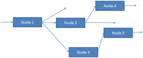
One type of multiple-node system for which most of the previous single-node results have an equivalent is referred to as a “rooted directed tree”. These are systems with only one entry point, no merging, no repeat visits, and for practical cases a finite number of nodes. Figure 1 shows a typical small example.

Figure 1. A typical (small) directed tree.

Note first of all that the finite number of nodes and no repeat visits mean that there are only a finite number of patient pathways, each of which can be used to define a type of patient with a specific set of requirements. As in single-node systems, the unlimited numbers of servers at each node means that each patient of each type proceeds along their pathway independently of all other patients.

If the interest is to model the total occupancy of the network of nodes, then this can be formulated as a single-node system, where patient types are defined according to the route that they follow, and each type of patient’s service time is their total service time across all the nodes that they visit. In theoretical terms, the probability distribution of total service time will be the convolution of the distributions of the individual node service times, whereas empirically one might estimate the distribution directly from total service time data. In either case results, 2.1.4(i)-(iii) can again be applied.

If the interest is to model the occupancy of one of the nodes (say node 3 in the simple example of Figure 2), then the state of interest (s) for any patient is occupancy of node 3. This can also be tackled using results 2.1.4(i)-(iii), again defining patient types according to the route that they follow. Only patient types whose route includes node 3 can contribute to its occupancy, so in the simple example, this is just the patient types following routes 1-3-5 and 1-2-3-5. For the first of these types: $$p_3\left(r,u,t\right)=\mathit{prob}\left[\left(\mathit{combined}\mathrm{ }\mathit{service}\mathrm{ }\mathit{time}\mathrm{ }\mathit{at}\mathrm{ }\mathit{nodes}\mathrm{ }1\mathrm{ }\&\mathrm{ }3\right)\ge \left(t-u\right)\right]-\mathit{prob}\left[\left(\mathit{service}\mathrm{ }\mathit{time}\mathrm{ }\mathit{at}\mathrm{ }\mathit{node}\mathrm{ }1\right)\ge \left(t-u\right)\right]$$

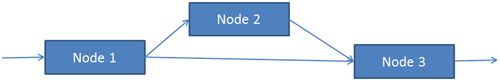
Figure 2. A simple tree with merging.

And for the second of these types: $$p_3\left(r,u,t\right)=\mathit{prob}\left[\left(\mathit{combined}\mathrm{ }\mathit{service}\mathrm{ }\mathit{time}\mathrm{ }\mathit{at}\mathrm{ }\mathit{nodes}\mathrm{ }1,\mathrm{ }2\mathrm{ }\&\mathrm{ }3\right)\ge \left(t-u\right)\right]-\mathit{prob}\left[\left(\mathit{combined}\mathrm{ }\mathit{service}\mathrm{ }\mathit{time}\mathrm{ }\mathit{at}\mathrm{ }\mathit{nodes}\mathrm{ }1\mathrm{ }\&\mathrm{ }2\right)\ge \left(t-u\right)\right]$$

As above, probability distributions for combined service times can be obtained as convolutions of the component distributions, or estimated directly from data on combined service times. In either case, results 2.1.4(i)-(iii) can again be applied.

2.4.2. More complicated networks

Once a network goes beyond the restrictions of a rooted directed tree, a variety of problematic issues can arise, including multiple entry points, merging of pathways and multiple visits to nodes. Figure 2 shows a simple example of a tree with merging, which can be considered as having two types of patient, who take the routes 1-2-3 and 1-3, respectively.

If the numbers arriving of the two types of patient are independent, then by results 2.1.4(i)-(iii) they will give rise to independent distributions of numbers of each type at each node, which can be combined in the usual ways.

However, if numbers of arrivals of the two patient types are not independent, very different results can occur. To take a simple example, suppose that lengths of stay at nodes 1, 2 and 3 are deterministic, spending 2 days at node 1, 2 days at node 2 (if needed) and 4 days at node 3. Six patients arrive at node 1 at time 0, each has a 0.7 chance of going via node 2, and our interest is in patients at node 3 on day 5. All the patients who go via node 2 will be at node 3 on day 5 and so will have a Bin(6,0.7) distribution, whilst all the patients who go direct to node 3 will also be at node 3 on day 5 and will have a Bin(6,0.3). However, these numbers of patients are clearly not independent, and in fact, their total is guaranteed to be 6 for this particular example. Hence this sort of scenario is not covered by results 2.1.4(i)–(iii), although in this case by careful consideration of the particular problem it has been possible to calculate the occupancy of interest.

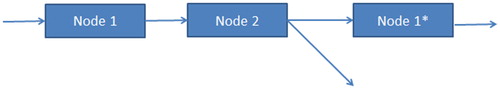
When some types of patients can return to a node, this can be modelled by introducing a dummy node, as shown in Figure 3 for a simple example where there are just two possible routes: 1-2 and 1-2-1*. In this case, each route can again define a type of patient whose location (including 1*) in the network can be modelled using results 2.1.4(i)–(iii). However, the numbers at node 1 and node 1* will not be independent, and so cannot be easily combined to give the distribution of the number of patients at the real node 1. Utley et al. (2009) speculate that methods for tackling issues such as this could be based upon using multinomial distributions to describe the probabilities of the same patients being in each or more than one location.

Figure 3. Using a dummy node for multiple visits.

Drawing on the influence of Massey and Whitt (1993) led Helm and van Oyen (2014) to propose a rather different way to deal with multiple-node networks. In particular, they argue that for predicting occupancy of a node (or a group of nodes), all that is needed to use results 2.1.4(i)–(iii) are the values of $p_s\left(r,u,t\right)$ for each patient type and for the node(s) of interest. Thus, the routes by which patients get to a node, or whether it is the first or a later visit, is immaterial to predicting the occupancy. Their approach relies on estimating the values of $p_s\left(r,u,t\right)$ from available data, rather than the more usual method involving combining routing probabilities and service time distributions, see Section 3.2 for further details.

2.4.3. Pseudocode for multiple-node infinite-server systems

As explained in the previous two sub-sections, quite a number of multiple-node systems can be tackled by a suitable choice of the state of interest in results 2.1.4(i)–(iii). Hence, the previous pseudocode is also directly applicable to these systems, with a suitable change of language to reflect the chosen definition of state of interest.

3. Healthcare applications

Healthcare applications to date of infinite-server queues have been dominated by studies of inpatient bed requirements, be it for a single ward, for multiple wards or for a whole hospital. However, there are also examples where the emphasis has been on staffing requirements, for example, in emergency departments, accident and emergency departments and community care. Modelling has been to support strategic, tactical and operational decision-making, and the models used have been time-homogeneous and time-inhomogeneous. In Section 3.1, we describe time-homogeneous models which are mainly used for strategic and tactical decision-making, and in Section 3.2, we describe time-inhomogeneous models which are used to support all three levels of decision-making.

3.1. Time-homogeneous models

Various authors have used time-homogeneous infinite-server models to address bed capacity issues in circumstances where it is believed that time-dependence of arrival rates are second order effects. By assuming random arrivals the well-known Erlang Loss formula, see for example Gross and Harris (1985), can be applied. This means that the steady-state probability that patients are turned away because all beds are full can be obtained simply from the truncated steady-state Poisson distribution of bed occupancy for the equivalent infinite-server system.

An early example is Bagust et al. (1999), writing in the British Medical Journal, who used a time-homogeneous model to demonstrate the implications of fluctuating and unpredictable demands for emergency admission for hospital management, and to quantify the daily risk of having insufficient beds. In fact, they chose to simulate the loss system rather than use the analytical Erlang loss formula, but the insights provided are the same. For a pool of 200 beds and the then current length of stay distributions, they showed that whilst average occupancy levels of 85% were likely to be achievable with relatively small numbers of patients turned away per year, a 90% occupancy level caused those numbers to grow dramatically.

In a later and more comprehensive paper, de Bruin, Bekker, van Zanten, and Koole (2010) first investigate how well the homogeneous Poisson arrivals assumption of the M/G/c/c model fits data collected on 24 clinical wards over a 3-year period. They found that Poisson distributions provided good fits for unscheduled patients, and more surprising they also showed good fits for scheduled patients for roughly half the wards, albeit at different levels for weekdays and weekends. They then argue that the M/G/c/c model provides an acceptable model for most wards, and demonstrate its use, including the Erlang loss formula, to help hospital managers judge acceptable occupancy levels for wards of different sizes and case mixes, and to estimate the benefits of merging operational units.

More recently, Monks et al. (2016), writing for a medical audience, used a three-node time-homogeneous infinite-server model to investigate capacity requirements for a stroke service comprising of an acute stroke unit, a rehabilitation unit and early supported discharge. They combine simulated infinite-server results with the Erlang Loss formula to estimate delay probabilities for patients needing acute beds and for patients needing rehabilitation beds under different scenarios, including current service, pooling (or partial pooling) of the acute and rehabilitation beds, and changes in the throughput of patients.

In a similar time-homogeneous vein, but considering elective patients, Gallivan et al. (2002) present results for an infinite-server model with constant daily arrivals of scheduled patients and a general distribution of length of stay. Also writing for a medical audience, their results comparing the distribution of bed demand with capacity clearly show how variability in length of stay contributes to variability in bed occupancy, and that the introduction of booked admissions would be unlikely to enable wards to operate at substantially increased bed occupancy levels. They also highlight and discuss the important issue of model complexity in this context. Infinite-server models deliberately do not attempt to include details of what might happen in practice in the event of bed requirements exceeding bed availability. They argue that attempting to do so might well overcomplicate the model, and that “…models do not need to replicate the full complexity of hospital operation to provide useful insights….” and “….models that attempt to do so can hinder understanding with confusing and irrelevant detail”.

3.2. Time-inhomogeneous models

A second area of application involves the use of time-inhomogeneous infinite-server queues to tackle the “hospital admission scheduling problem”, i.e., essentially tailoring admission schedules to make good use of available beds. There are two versions of how this task can be tackled. Version 1 is to simply use the infinite-server models to predict the bed usage of any admission schedule that is being considered, version 2 combines the predictive model with an optimisation algorithm intended to find the “best” admission schedule.

An early example of version 1, i.e., predictive modelling, is Utley et al. (2003), who assume time-dependent arrivals in discrete time to represent both scheduled and unscheduled admissions. Their formulation corresponds to a particular case of model 2.1.4(iii) in which the two types of arrival (R = 2) are scheduled and unscheduled. The numbers of scheduled arrivals are assumed to be deterministic and can differ by day of the week. Each arrival has a fixed probability of not attending, and a common length of stay distribution is assumed. The number of unscheduled arrivals have a general distribution, which can differ by day of the week, and they are assumed to have the same length of stay distribution as the scheduled patients. Their results include formulae for the steady-state mean and variance of bed demand for each day of the week for any assumed admission schedule. They demonstrate their results on data based upon a cardiac surgery department; and using the central limit theorem to justify the use of the normal distribution they calculate probabilities of daily demand exceeding bed capacity. As with Gallivan et al. (2002), they deliberately make no attempt to model what might happen if demand exceeds capacity.

Utley, Jit, and Gallivan (2008) use essentially the same infinite-server models to investigate a policy issue associated with the possible introduction of treatment centres. In theory, treatment centres have the potential to be more efficient than normal wards because they concentrate on homogeneous subsets of patients, and so reduce the variability in lengths of stay. Based on data for UK urology inpatient services, they use a range of scenarios to show how increases in efficiency may well be small or indeed not possible. Difficulties in achieving efficiencies are shown likely exist if only one or two hospitals are served by the treatment centre, and/or numbers of emergency patients are high, and/or the treatment centre patients turn out to be less homogeneous than intended.

Bekker and de Bruin (2010) use predictive models for continuous time-inhomogeneous infinite-server systems to investigate capacity planning issues for clinical wards. Like de Bruin et al. (2010) they argue that important insights can be obtained by making the simplifying assumption that both scheduled and unscheduled arrivals can be represented as Poisson. Making a further assumption of hyper-exponential distributions of length of stay, they go on to use analytical M(t)/H/∞ models combined with two different approximations (approximate Erlang loss formula and the square root staffing rule) to demonstrate how the impact of weekly fluctuations in arrival rates can have serious implications for the required bed capacity for clinical wards. They also go on to show how within day fluctuations in arrival rates can often be ironed out in this setting, but that they become important when setting staffing levels in an emergency department.

In the first approximation, they assume that arrivals are lost when beds are full (rather than attempt to model queueing patients or early discharges), and hence that performance is represented via a loss probability. This they estimate by applying the modified-offered-load approximation of Massey and Whitt (1994), which applies the steady-state Erlang loss formula with traffic intensity replaced by the time-dependent bed demand. Algorithms to improve upon this approximation for the case of exponential service times, see Alnowibet and Perros (2009), and for more general service times, see Izady and Worthington (2011), are now available.

In the second approximation, they highlight the potential value of using the square root staffing rule, a heuristic rule based on the work of Jennings, Mandelbaum, Massey, and Whitt (1996). The rule is usually associated with call centre staffing models, assumes Poisson arrivals and approximates the resulting Poisson distribution of demand by a Normal distribution to guide the extent to which staffing levels should exceed the time-dependent expected demands levels.

The applications of time-inhomogeneous models described so far have been concerned with strategic or tactical decisions about resourcing and/or patient scheduling. However, the same predictive time-dependent equations apply equally well for short-term planning decisions. Pagel et al. (2017) describe their use for forecasting the short-term demand for beds in an intensive care unit (ICU). Given their aim to forecast bed requirements in the next few days, they need to extend the standard formulation incorporating emergency and elective patients by adding a third type of patient, namely those patients already in the ICU. A further interesting feature of this paper is its description of the implementation of this model, and an evaluation of the implementation over a period of more than 3 years.

Gallivan and Utley (2005) develop a version 2 model, i.e., an optimisation approach, for the hospital admission scheduling problem. Their first step is a version 1 model providing analytic expressions for mean and variance of bed demand. The model they use is very similar to that of Utley et al. (2003), generalised to include patient types (e.g. defined by health-related groups) and simplified a little to assume Poisson unscheduled arrivals. After some discussion of possible optimisation criteria, they propose a linear programming (LP) formulation derived from road traffic modelling which minimises the maximum daily traffic intensities, subject to achieving target admission rates of patients of the different types. They demonstrate the approach on an example problem, based on a 32-bedded orthopaedic centre, which gives rise to a small LP problem, and suggests that the same approach could work well for significantly bigger and more detailed formulations.

Also important is their recognition that their LP formulation only approximates the “real” problem. In particular, the traffic intensities they use in their assumed objective and the admission levels they use in their assumed constraints are linear functions of scheduled admissions (i.e., the decision variables), hence enabling their LP formulation, whereas the probability of demand exceeding bed capacity (which more closely mirrors real management objectives or constraints) is not linear in the decision variables. Clearly, a “perfect” model would need to deal with this sort of nonlinearity, alongside recognition that the infinite-server formulation itself deliberately omits detailed modelling of how particular hospitals might deal with situations where demand exceeds capacity.

Isken et al. (2011) develop and apply methods based on the single-node results of Gallivan and Utley (2005) to tackle bed occupancy modelling and procedure scheduling for an obstetrics department consisting of four distinct units, and hence four nodes. Their formulation involves 11 patient types, each with specific requirements, and hence well-specified routes through the four nodes, with no repeat visits. However, rather than use the multi-node results described in Section 2.4, they assume that transfers of scheduled admissions between nodes can be represented as deterministic processes and hence they use single-node results to provide approximate formulae for the means and variances of daily bed demands at each node. Using their single-node results they then go on to propose an LP formulation based on smoothing daily occupancies, and a non-linear formulation which uses a normal approximation for the probabilities that daily demands exceed capacities.

Two further interesting features of their work are the development of open source software tools to implement their models, and the use of simulation models to attempt to validate some of the approximations that they use.

Presenting a more rigorous treatment of multi-node systems, Helm and van Oyen (2014) tackle the whole hospital admission scheduling problem in which each ward is represented by a node. They measure hospital performance in terms of throughputs, off-ward boarding of patients (i.e., when patients are diverted to other wards because their intended ward is full) and refused admissions (i.e., when admissions are refused because the hospital is full). In order to do so, they develop two stochastic location models, PALM (Poisson arrival-location model) and d-CALM (deterministic controlled-arrival-location model) to provide the values of $p_s\left(r,u,t\right)$ for each patient type and each node which are needed to use results 2.1.4(i)-(iii). They assume time-inhomogeneous Poisson arrivals of non-elective patients and day-of-week-dependent deterministic arrivals of elective patients, leading to expressions for the means of the Poisson distributions of the non-elective bed demands and for the means and variances of elective bed demands by ward and day.

In order to formulate a hospital-wide optimisation problem that is linear in its decision variables (essentially the daily throughputs of different patient types), they introduce linearised approximate expressions for their “blocking” probabilities, i.e., the probabilities that demands for each ward exceed their capacities, and the probability that total demand exceeds hospital capacity. They provide two formulations, one which maximises the weighted sum of throughputs of elective patients subject to constraints on the approximate blocking probabilities, and the second controlling blocking probabilities subject to achieving desired throughputs. As noted earlier, an important extra feature of their paper is the development of a practical approach for estimating values of $p_s\left(r,u,t\right)$ directly from available data, given that the directly observable behaviour of patients is influenced by the non-availability of beds whereas the values of $p_s\left(r,u,t\right)\mathrm{ }$that are required the need to be unaffected by bed availability. Hence, an important and innovative part of their paper is the development of a statistical approach capable of providing unbiased estimates of these probabilities. However, because it is a purely statistical approach, it does not naturally enable the probabilities to be updated to reflect actions that management might take.

Moving away from healthcare applications focussed on inpatient beds, Utley et al. (2009) develop predictive results for multimode systems of a “directed rooted tree” type in order to tackle the problem of estimating demand for community health services. In this work, nodes represent the state that a patient is in, which could be a physical location, or a type of therapy, a health condition, or a combination thereof. They assume general independent time-inhomogeneous distributions of arrivals in discrete time and general sojourn time distributions for each service to give time-dependent expressions for the means and variances of demand levels for each service. They illustrate the approach by predicting the growth of demand during the first year of a newly configured community service for people with common mental health problems. Following the spirit of earlier work, this information on “unfettered” demand can be used to guide capacity-related decisions.

Another area for healthcare applications is emergency departments where, as noted by Bekker and de Bruin (2010), the within-day variations in demand can be important for deciding staffing levels. Izady and Worthington (2012) formulate a UK accident and emergency department (AED) as a time-inhomogeneous network of finite server queues with Poisson arrivals (which they simulate), but use an analytic infinite-server multimode model combined with the square root staffing law to guide the hourly staffing levels of different types in the different service areas within the AED. The value of the infinite-server model here is to provide a heuristic to narrow down from a very large number of possibilities the staffing patterns worth simulating in order to find an efficient way to achieve waiting time targets.

Tan et al. (2013) also consider an emergency department setting in which they consider hourly staffing levels of doctors in two main areas (resuscitation/critical care and ambulatory care), but with the added features of (i) switching staff between the areas and (ii) patients having multiple movements between the areas. Their particular interest is to show the potential benefit of dynamic allocation of staff, in particular, switching doctors between the two areas based on real-time modelling of demand levels. Using infinite-server simulation models and heuristics based on the square root staffing law they design and evaluate static staffing schedules and dynamic staffing patterns, using historic arrival patterns for the former and historic and real-time arrivals for the latter. Their use of simulation models instead of analytical models brings with it some of the extra challenges associated with simulation optimisation, see, for example, Fu (2014) for an intensive introduction to simulation optimisation.

4. Future developments

Three directions for future developments are described here. The first direction is essentially new healthcare problems tackled using existing infinite-server models, the second is healthcare problems for which new infinite-server model development is required, the third is new ways of using infinite-server models (old and new) in combination with other models.

4.1. New applications of existing models

Existing models have mainly been used to inform strategic or tactical decision-making concerning major hospital resources for which arrival patterns, service times and routing probabilities are well established (with appropriately stable historic data) and/or subject to control. As data increasingly become available for a greater range of services in hospitals or in the community, there will be scope for addressing their strategic or tactical resourcing decisions as well.

A second data development is the growing amount of real-time data becoming available in healthcare, offering the scope for more operational resource allocation decisions to be underpinned by system modelling. The analytical nature of many infinite-server models and their associated short runtimes will be an advantage in this respect. The work of Pagel et al. (2017) on short-term predictions of ICU bed demands is an early example of this sort of work.

A third type of new application might stem from the scope for creative interpretations of the concept of a model that predicts the occurrence of “problems” or “pressure”, without any attempt to model the precise consequences of that pressure. For example, Suen (2015) shows how infinite-server models can be used to create convenient and insightful performance indicators to compare the performance of hospitals in a way that allows for their differing mixes of patients.

4.2. Healthcare problems requiring new infinite-server model developments

A key characteristic of healthcare applications of infinite-server models has been the assumed independent arrivals of different patient types and the assumption that patients progress through the service (or network of services) independently once they have arrived. Hence for cases where arrivals of patient types, either on the same day or on different days of the week, are correlated new model developments are required. Also, as outlined in Section 2.4.2, for cases where the network cannot be described as a rooted directed tree, the assumption of independence of travel breaks down and more work is required to develop appropriate modelling approaches.

Some interesting early work on some aspects of non-independence is described in Fakinos (1984) who considers infinite-server systems where arrivals occur in groups, and where the within-group service times are allowed to be dependent. Assuming that arrivals are generated by a non-homogeneous compound Poisson process (i.e., groups arrive as a non-homogeneous Poisson process, with group size having a known distribution), Fakinos uses probability generating functions to show that the number in the system at time t will have a compound Poisson distribution (i.e., number in the system can be seen as being made up of groups of individuals, where the number of groups is Poisson and the distribution of group sizes is known). Note that the mean of the Poisson distribution and the probability distribution of group sizes are derived from the parameters of the arrival process and the joint distributions of service times associated with the groups of arrivals of different sizes. Economou and Fakinos (1999) later show that the same approach can be extended to the case where there can be more than one type of customer in a group of arrivals, with each customer type having their own service time characteristics.

4.3. Combining infinite-server models with other models

Multi-fidelity modelling is a phrase that is more common in engineering than in management science but is one that encompasses key issues for the application of models in management decision-making. In engineering, a high fidelity model would often be a model that is accurate enough for its intended purpose but requiring a high computational cost; whereas a low fidelity model would have a lower computational cost but would not have the desired accuracy. In such circumstances, there can be scope for using the low fidelity model to, in some sense, narrow down the problem or solutions of interest, before using the high fidelity model to come to a final decision. Note that this concept goes beyond the merits of longer run lengths to achieve greater statistical accuracy common in simulation studies, and is concerned with the level of detail included in the model, and its consequential need for greater computational effort.

Xu, Lee, and Celik (2014) develop this principle in a management science simulation modelling setting, using a simple example of a manufacturing process to demonstrate the concept and the nature of results. They describe the principle as using a low fidelity simulation model to provide a preliminary comparison of all the possible options, before using a high fidelity simulation model to choose amongst the options that the low fidelity model identifies as most promising. Where the low fidelity model is an analytical model (as for the infinite-server models) rather than a simulation model, the scope for computational savings, and hence the potential advantage of the approach, is even greater.

A significant challenge for multi-fidelity modelling is the requirement that the low fidelity model is capable of ordering potential solutions sufficiently well that those identified as high performers according to the low fidelity model will also be high performers according to the high fidelity model. The fact that infinite-server models reflect many of the important characteristics known to be important in the solution of the real-life problems strengthens the likelihood that the required correlation will be present. The application of infinite-server models by Izady and Worthington (2012) to Accident and Emergency staffing patterns has some of these characteristics. Although they did not use their low fidelity model to consider all possible solutions, they nevertheless used it to find solutions that were going to be markedly better than existing staffing patterns.

Chow, Puterman, Salehirad, Huang, and Atkins (2011) provide a variation on the above theme which is interesting in a number of respects. Their low fidelity model is a mixed integer programming model designed to schedule surgical admissions so as to stabilise expected bed occupancies. This is then used alongside a (high fidelity) infinite-server simulation model to more accurately predict the likely stochastic consequences of schedules identified as “good” by the mixed integer programming model. As with some previous examples, the simulation model of the infinite-server system could, in theory, be replaced by an analytical model, however, in some circumstances, the simulation representation is quite convenient. Finally, the choice of an infinite-server model as a high fidelity model emphasises that the high fidelity model could well itself be an approximation of the real situation, but one that is deemed accurate enough for the intended purpose. Clearly, infinite-server models have the potential to take on a number of roles in situations where multi-fidelity models are being considered.

5. Summary

Infinite-server queueing models have a well-established track record in being used via the concept of offered load in healthcare applications. The mathematical approaches developed which underpin this work have taken a variety of forms, each with their own set of assumptions and notations. However, they are all centred around the concept of independence of travel which is guaranteed by the assumption of infinite servers. The first part of this paper has therefore been to consolidate the approaches and results used in this work in a form that is intended to be easily understood and easily applied by operational researchers interested to use them or to develop further results. Pseudocode for implementing the central set of results is also included to further facilitate such work.

The second part of the paper has reviewed, in terms of the consolidated theory, healthcare applications ranging from capacity planning for hospital wards to staff scheduling in A&E through to admission scheduling to smooth inpatient workloads. Some applications have used infinite-server models in a purely predictive sense, whereas others have integrated the predictions into optimisation formulations in an attempt to find optimal solutions, e.g. admission schedules. Most of the early examples concentrated on tackling strategic decisions and made use of historical data, whereas some more recent examples have looked at more operational decisions and have occasionally made use of near real-time data. In some cases, modellers have found it adequate to use time-homogeneous formulations whilst others have chosen to use time-inhomogeneous formulations.

This review then leads to the identification of three general directions for further work. New applications of existing models could be achieved simply by greater awareness of, and access to, the infinite-server modelling concepts and methods. Increasing data availability across a wider set of services in hospitals and in community service, some of it real-time data, should also contribute to this larger set of applications, including more support for operational decision-making. There is also scope for more creative uses of the ethos of infinite-server models, i.e., they use relatively simple models to indicate the pressure a system is under, and avoid the much more complicated (or impossible) task of modelling the consequences of that pressure.

The second general direction concerns new infinite-server model development. In particular, this needs to concentrate on approaches to deal with arrival patterns within which numbers of different types of patients cannot be considered as independent and also on approaches to deal with networks of services which cannot be described as a rooted directed tree.

The third general direction is, in fact, the arena of multi-fidelity modelling in which the natural analytical characteristics of infinite-server models seem particularly well suited to providing insightful and inexpensive low fidelity models to be used in combination with more expensive high fidelity models.

In summary, despite their unrealistic assumption of infinite resources, and hence their inability to directly model queues and queueing times, infinite-server queueing models have played an important role in supporting healthcare resourcing decisions, often via the offered load concept. Our hope is that consolidating the existing theory in an accessible form, providing a review of existing applications and identifying three directions for new work will enable further applications of the existing theory, and guide further developments of applicable theory.

Disclosure statement

No potential conflict of interest was reported by the authors.

Additional information

Funding

This work was funded by the Engineering and Physical Sciences Research Council [EP/H023151/1 STOR-i centre for doctoral training].

References

- Alnowibet, K., & Perros, H. (2009). Nonstationary analysis of the loss queue and of queueing networks of loss queues. European Journal of Operational Research, 196(3), 1015–1030. doi: 10.1016/j.ejor.2007.10.066
- Bagust, A., Place, M., & Posnett, J. W. (1999). Dynamics of bed use in accommodating emergency admissions: Stochastic simulation model. British Medical Journal, 319(7203), 155–158. doi: 10.1136/bmj.319.7203.155
- Bekker, R., & de Bruin, A. M. (2010). Time-dependent analysis for refused admissions in clinical wards. Annals of Operations Research, 178(1), 45–65. doi: 10.1007/s10479-009-0570-z
- Chow, V. S., M. L., Puterman, N., Salehirad, W., Huang, & Atkins, D. (2011). Reducing surgical ward congestion through improved surgical scheduling and uncapacitated simulation. Production and Operations Management, 20(3), 418–430. doi: 10.1111/j.1937-5956.2011.01226.x
- de Bruin, A. M., Bekker, R., van Zanten, L., & Koole, G. M. (2010). Dimensioning hospital wards using the Erlang loss model. Annals of Operations Research, 178(1), 23–43. doi: 10.1007/s10479-009-0647-8
- Economou, A., & Fakinos, D. (1999). The infinite server queue with arrivals generated by a non-homogeneous compound Poisson process and heterogeneous customers. Stochastic Models, 15(5), 993–1002.
- Eick, S. G., Massey, W. A., & Whitt, W. (1993). The physics of the Mt/G/∞ queue. Operations Research, 41(4), 731–742. doi: 10.1287/opre.41.4.731
- Fakinos, D. (1984). The infinite server queue with arrivals generated by a non-homogeneous compound Poisson process. Journal of the Operational Research Society, 35(5), 439–445. doi: 10.1057/jors.1984.85
- Fu, M. C. (2014). Handbook of simulation optimization. M. C. Fu (Ed.), New York: Springer.
- Gallivan, S. (2005). Mathematical methods to assist with hospital operation and planning. Clinical and Investigative Medicine, 28(6), 326–330.
- Gallivan, S., & Utley, M. (2005). Modelling admissions booking of elective inpatients into a treatment centre. IMA Journal of Management Mathematics, 16(3), 305–315. doi: 10.1093/imaman/dpi024
- Gallivan, S., Utley, M., Treasure, T., & Valencia, O. (2002). Booked inpatient admissions and hospital capacity: Mathematical modelling study. BMJ, 324(7332), 280–282. doi: 10.1136/bmj.324.7332.280
- Gross, D., & Harris, C. M. (1985). Fundamentals of queueing theory (2nd ed.), Hoboken, NJ: Wiley.
- Helm, J. E., & Van Oyen, M. P. (2014). Design and optimization methods for elective hospital admissions. Operations Research, 62(6), 1265–1282. doi: 10.1287/opre.2014.1317
- Isken, M. W., Ward, T. J., & Littig, S. J. (2011). An open source software project for obstetrical procedure scheduling and occupancy analysis. Health Care Management Science, 14(1), 56–73. doi: 10.1007/s10729-010-9141-8
- Izady, N., & Worthington, D. (2011). Approximate analysis of non-stationary loss queues and networks of loss queues with general service time distributions. European Journal of Operational Research, 213(3), 498–508. doi: 10.1016/j.ejor.2011.03.029
- Izady, N., & Worthington, D. (2012). Setting staffing requirements for time dependent queueing networks: The case of accident and emergency departments. European Journal of Operational Research, 219(3), 531–540. doi: 10.1016/j.ejor.2011.10.040
- Jennings, O. B., Mandelbaum, A., Massey, W. A., & Whitt, W. (1996). Server staffing to meet time-varying demand. Management Science, 42(10), 1383–1394. doi: 10.1287/mnsc.42.10.1383
- Massey, W. A., & Whitt, W. (1993). Networks of infinite-server queues with nonstationary Poisson input. Queueing Systems, 13(1–3), 183–250. doi: 10.1007/BF01158933
- Massey, W. A., & Whitt, W. (1994). An analysis of the modified offered load approximation for the Erlang loss model. The Annals of Applied Probability, 4(4), 1145–1160. doi: 10.1214/aoap/1177004908
- Mitrani, I. (1998). Probabilistic modelling. Cambridge: Cambridge University Press.
- Monks, T., Worthington, D., Allen, M., Pitt, M., Stein, K., & James, M. (2016). A modelling tool for capacity planning in acute and community stroke services. BMC Health Services Research, 16(1), 530 doi: 10.1186/s12913-016-1789-4
- Newell, G. (1966). The M/G/∞ queue. SIAM Journal on Applied Mathematics, 14(1), 86–88. doi: 10.1137/0114007
- Pagel, C., Banks, V., Pope, C., Whitmore, P., Brown, K., Goldman, A., & Utley, M. (2017). Development, implementation and evaluation of a tool for forecasting short term demand for beds in an intensive care unit. Operations Research for Health Care, 15, 19–31. http://dx.doi.org/10.1016/j.orhc.2017.08.003
- Palm, C. (1943). Intensity variations in telephone traffic. Ericsson Technics, 44, 1–189 (in German), (English translation by North Holland, Amsterdam, 1988).
- Suen, D. (2015). The development and application of an analytical healthcare model for understanding and improving hospital performance (Doctoral dissertation). Lancaster University, Lancaster.
- Tan, K. W., Tan, W. H., & Lau, H. C. (2013). Improving patient length-of-stay in emergency department through dynamic resource allocation policies, IEEE International Conference on Automation Science and Engineering (CASE), 984–989.
- Utley, M., Gallivan, S., Pagel, C., & Richards, D. (2009). Analytical methods for calculating the distribution of the occupancy of each state within a multi-state flow system. IMA Journal of Management Mathematics, 20(4), 345–355. doi: 10.1093/imaman/dpn031
- Utley, M., Gallivan, S., Treasure, T., & Valencia, O. (2003). Analytical methods for calculating the capacity required to operate an elective booked admissions policy for elective inpatient services. Health Care Management Science, 6(2), 97–104.
- Utley, M., Jit, M., & Gallivan, S. (2008). Restructuring routine elective services to reduce overall capacity requirements within a local health economy. Health Care Management Science, 11(3), 240–247.
- Weiss, N. A., Holmes, P. T., & Hardy, M. (2006). A course in probability. Boston, MA: Pearson Addison Wesley.
- Whitt, W. (2016). Queues with time-varying arrival rates: A bibliography. Working paper. New York: Columbia University.
- Worthington, D. (2009). Reflections on queue modelling from the last 50 years. Journal of the Operational Research Society, 60(suppl. 1), S83–S92. doi: 10.1057/jors.2008.178
- Xu, J., Lee, L. H., & Celik, N. (2014). Efficient multi-fidelity simulation optimization. Proceedings of the 2014 Winter Simulation Conference, 3941–3951.