Financial volatility modeling with option-implied information and important macro-factors

Abstract

The research debate on the informational content embedded in option prices mostly approves the incremental predictive power of implied volatility estimates for financial volatility forecasting beyond that contained in GARCH and realized variance models. Contributing to this ongoing debate, we introduce the novel AIM-HEAVY model, a tetravariate system with asymmetries, option-implied volatility, and economic uncertainty variables beyond daily and intra-daily dispersion measures included in the benchmark HEAVY specification. We associate financial with macroeconomic uncertainties to explore the macro-financial linkages in the high-frequency domain. In this vein, we further focus on economic factors that exacerbate stock market volatility and represent major threats to financial stability. Hence, our findings are directly connected to the current world-wide Coronavirus outbreak. Financial volatilities are already close to their crisis-peaks amid the generalized fear about controversial economic policies to support societies and the financial system, especially in the case of the heavily criticized UK authorities’ delayed and limited response.

Keywords:

• Economic policy uncertainty
• high-frequency data
• implied volatility
• macro-financial linkages
• realized variance
• risk management

1. Introduction

Financial volatility is widely recognized as one of the most significant inputs for any asset valuation task. On the one hand, market practitioners rely on robust volatility modeling to generate efficient up-to-the-minute forecasts of future volatility, required for day-to-day decisions on asset allocation, market risk hedging, derivatives pricing, capital budgeting, or any risk assessment consideration in the operations management context (see, for example, Benati, 2015; Cesarone & Colucci, 2018; Datta et al., 2007; Tan, 2002). On the other hand, policymakers consider financial market volatility as a barometer of the whole financial system and economy’s vulnerability. Motivated by the tremendous need for reliable estimates of subsequent volatility, academics have delved deeply into formalizing several volatility metrics and developing forecasting models, addressing a number of empirical features of the returns time series second moment.

Given that return volatility is unobservable, one requires first a proxy of this latent process. Daily squared returns and realized variance (computed on intra-daily observations) are the most popular measures of ex-post asset returns dispersion. An enormous amount of empirical literature has been investigating the forecasting ability of the conditional variance models for returns through the GARCH-type specifications and the long memory conditional mean models for the realized measures. Starting from Bollerslev (1986) with the introduction of GARCH models for daily returns conditional variance, the GARCH family expanded to cover numerous stylized facts of the financial time series’ volatility pattern, such as leverage (e.g. see Glosten et al., 1993) and long memory (e.g. see Baillie et al., 1996), among others, and even utilize truncated distributions for stock price limits (e.g. Adcock et al., 2019). Following the first studies that formalized the daily realized measures on intra-daily returns (e.g. the realized variance established by Andersen et al., 2001, and the realized kernel by Barndorff-Nielsen et al., 2008), Andersen et al. (2001) and Corsi (2009) proposed long memory models for the conditional mean of the realized variance, that is the ARFIMA and HAR specifications, respectively.

In order to improve the forecasting accuracy of the various volatility models, econometricians have developed specifications combining daily with intra-daily measures. Engle (2002) estimated the daily GARCH-X specification adding the realized measure as an exogenous variable in the GARCH(1,1) equation to capture the incremental information of the higher-frequency domain. Accordingly, Shephard and Sheppard (2010) introduced the HEAVY (High-frEquency-bAsed VolatilitY) framework and Hansen et al. (2012) followed with the Realized GARCH (see also Barunik et al., 2016). Both HEAVY and Realized GARCH jointly estimate daily returns’ conditional variance and realized measure’s conditional mean. The HEAVY system of equations is proved to adopt to information arrival more rapidly than the classic daily GARCH process. A key advantage is the system’s robustness to certain forms of structural breaks, especially during crisis periods, since the mean reversion and short-run momentum effects result in higher quality performance in volatility level shifts and more reliable forecasts (Shephard & Sheppard, 2010).

Apart from volatility modeling based on historical information, that is daily returns conditional variance and realized variance on intra-daily observations, there is another vein of research that employs the standard deviation extracted from option prices. Implied volatility is an ex-ante volatility proxy, that is more forward-looking since it captures the market’s forecast for volatility over the life of the option. This market-determined measure is widely believed to contain incremental information from options market participants and, therefore, superior predictive power for future volatility compared to historical information. Blair et al. (2001), Martens and Zein (2004), Frijns et al. (2010), and Busch et al. (2011) are among the huge variety of studies providing clear evidence in favor of the significant informational content in option-inferred standard deviation that yields remarkably lower forecasting errors in financial volatility predictions than historical time series models (either daily GARCH or realized variance autoregressive models).

In this paper, motivated by the merits of the HEAVY framework and the established body of work assessing the implied volatility superiority in volatility forecasting, we examine the inclusion of the ex-ante volatility proxy in the bivariate system of ex-post squared returns and realized variance equations on seven US and European stock index data. We first augment the bivariate benchmark specification with asymmetries through the structure of the GJR-GARCH (Glosten et al., 1993) which considerably improves Bollerslev’s model. One of our main findings in the asymmetric specification is that the conditional variance of returns and the conditional mean of the realized variance are significantly affected by the leverage effects from both variables, that is, squared negative returns and negative signed values of realized variance. Secondly, we test the informational role of implied volatility in modeling the returns conditional variance and the realized measure. We find that options market-determined variances are mostly better predictors of both ex-post volatility measures and conclude that the best volatility modeling framework is a trivariate system with asymmetries and all three variables: squared returns, realized and implied variances. In other words, we extend the bivariate Asymmetric model to the trivariate Asymmetric-Implied HEAVY specification which outperforms the former.

Thirdly, inspired by the importance of the macro-financial linkages, we explore the possible macro-effects on the financial volatility patterns by adding a fourth variable to the system, namely the daily Economic Policy Uncertainty index for the US and the UK (Baker et al., 2016). Our macro-risk factor added, apart from capturing the macro-impact, is also a sentiment proxy of the overall economic risks perception ubiquitous in the society and each economic agent separately. Such perceptions alongside volatility predictions are widely proved to be significant for any management decision process. The macro-augmented tetravariate system further improves the out-of-sample performance of our models providing evidence that macro-uncertainty contains a significant amount of information for predicting financial market volatility. Finally, we focus on the macro-financial linkages in the high-frequency domain by including additional macro-factors in the realized volatility equation of the tetravariate system and by investigating the destabilizing uncertainty effect on the various macro-financial parameters. The central finding obtained from the realized variance macro-analysis shows that higher credit risk pricing, financial stress risk, commodity values, unemployment, and inflation uncertainty exacerbate ex-post volatility. At the same time, our sensitivity analysis indicates that higher uncertainty magnifies the asymmetric and macro-effects on the realized measure, confirming the conclusion of Karanasos and Yfanti (2020) for the UK uncertainty destabilizing ramifications on European stock market volatility.

The present study aims at contributing to the existing empirical literature in three ways. First, we build on the successful HEAVY methodology for volatility forecasting to improve the volatility modeling framework by combining the conditional variance of daily returns with the leverage effect, the ex-post volatility realized measure on inter-period information, and the ex-ante implied volatility from option markets’ superior predictive content. The wide variety of the extant empirical studies mostly compares implied volatility with realized variance for conditional variance forecasting or implied volatility with daily squared returns to predict future realized variance, considering or ignoring asymmetries. To the best of our knowledge, we are the first to provide a complete system of equations with all three dispersion measures and demonstrate that this is the preferred specification over any bivariate combination in terms of both in- and out-of-sample performance. Existing studies conclude on the superiority of one sole measure to forecast the other one. Second, beyond forecasting the daily returns conditional variance and the realized measure which is the main research topic in existing literature, we investigate the dynamics of implied volatility per se which is a research challenge mostly overlooked by financial econometricians. Reliable implied volatility forecasts are of paramount importance for market practitioners in options trading and any other finance task that requires the volatility input, as well. The forecastability of market-determined volatility is only explored by a few papers applying autoregressive processes with or without long memory features (Dunis et al., 2013; Fernandes et al., 2014; Konstantinidi et al., 2008). In this study, we forecast implied volatility in the trivariate system where the best model includes first-order autoregressive terms associated with returns leverage effects, in many cases.

Our final contribution is the macro-extension of the trivariate system following Karanasos and Yfanti (2020) who have considered the macro-financial linkages in the high-frequency domain. Given that volatility in financial markets represents financial uncertainty, we attempt to associate it with the other type of uncertainty coming from the macroeconomic perspective. We include the daily Economic Policy Uncertainty index as the fourth endogenous variable in the tetravariate system and not as an exogenous regressor of the realized variance equation proposed by Karanasos and Yfanti (2020), who work on a narrower context, namely the bivariate returns-realized measure system, and apply the macro-financial linkages aspect only on the latter volatility estimator. Interestingly, the macro-uncertainty is found to have a discernible impact on two of the three financial uncertainty metrics, namely the squared returns and the realized variance, without receiving any significant financial uncertainty effect from US and European stock markets. Economic uncertainty, besides other macro-factors, introduces new frictions in financial markets that should be incorporated in financial time series modeling to compute more accurate macro-informed volatility forecasts. Overall, we introduce the Asymmetric-Implied-Macro (AIM) HEAVY model and achieve a richer understanding of the volatility dynamics highly beneficial for both market practitioners and policymakers in any business finance operation and regulatory response.

Our study is further relevant to a highly topical issue nowadays, the world-wide Coronavirus outbreak. Market turbulence is already observed through markedly increased volatilities close to the peak reached during the 2008 global crisis. Markets are seriously afflicted by the generalized fear about controversial economic policies to support societies and the financial system, especially in the case of the heavily criticized UK government’s delayed and deficient response. Given an unprecedented and challenging threat, namely the rapidly contagious virus across the whole universe, economic agents feel uncertainty about future government policy choices, their implementation, and their potential impact as well. Even if they see officials assuring that Covid-19 harmful effects are manageable, skepticism, criticism, and loss of confidence are still there and fairly captured by the Economic Policy Uncertainty index levels.

The remainder of the paper is structured as follows. In Section 2, we present the econometric framework with the proposed HEAVY extensions. Section 3 describes the data and Section 4 analyzes the in-sample estimation results. The next section focuses on the macro-factors incorporated in the realized variance equation and studies the policy uncertainty effects across the macro and volatility parameters of the realized measure equation. Section 6 discusses the out-of-sample performance of the proposed models. Finally, Section 7 concludes the analysis.

2. The econometric framework

Building on the HEAVY framework by Shephard and Sheppard (2010) who combine two volatility estimators in a bivariate system, we further account for the downside risk in the volatility process through our first Asymmetric HEAVY extension of the returns-realized variance system. Following Pong et al. (2004) who found that historical volatility forecasting accuracy is attributed to the intra-daily information rather than long memory considerations of the modeling framework, we do not enrich the HEAVY system with long memory features. Similarly, we prefer to ignore power effects (through the APARCH model of Ding et al., 1993) in order to stick to the second moment modeling and forecasting without the complexity of mixed power transformations of the four conditional variances included that would impede straightforward economic interpretations. Moreover, we augment the bivariate system with a third variable, the implied volatility measure, to capture the incremental information content from stock index options market beyond that contained in daily and intra-daily returns. Likewise, we further combine the three financial uncertainty proxies with a macro-uncertainty index to estimate the tetravariate specification of returns, realized and implied variance, and economic policy uncertainty. The additional input from options-inferred variation and economic sentiment in the bivariate system will further improve the model’s forecastability beyond the improvement that would be achieved by long memory features (see, for example, Karanasos et al., 2020). Lastly, we focus on the realized variance equation where we add additional macro-regressors for credit risk, financial stress, commodity prices, unemployment, and inflation, and perform a sensitivity analysis of the policy uncertainty effects on the macro and volatility parameters that drive the dynamics of the realized measure.

2.1. Benchmark and asymmetric formulation

The benchmark HEAVY specification (Shephard & Sheppard, 2010) employs the close-to-close returns (r_t) and the realized measure of dispersion based on intra-daily quotes, RM_t. We calculate the signed square rooted (SSR) realized measure as follows: $\widetilde{R{M}_t}=$sign$(r_t)\sqrt{R{M}_t},$ where sign$(r_t)=1,$ if $r_t⩾0$ and sign$(r_t)=-1,$ if r_t < 0. We assume that the returns and the SSR realized measure are characterized by the following equations: (1) $$r_t=e_{rt}{\sigma }_{rt},\widetilde{R{M}_t}=e_{Rt}{\sigma }_{Rt},$$(1) where the stochastic term e_it is independent and identically distributed (i.i.d), $i=r,R;$ σ_it is positive with probability one for all t and it is a measurable function of ${\mathcal{F}}_{t-1}^{(XF)},$ that is the filtration generated by all available information through time t − 1. The ${\mathcal{F}}_{t-1}^{(HF)}$ (X = H) notation refers to the high-frequency past data, i.e. for the case of the realized measure, and ${\mathcal{F}}_{t-1}^{(\mathit{LoF})}$ (X = Lo) to the low-frequency past data, i.e. for the case of the close-to-close daily returns. For notational convenience, we will drop hereafter the superscript XF. The HEAVY model assumes zero mean and unit variance for e_it. Hence, the two variables have zero conditional means and conditional variances given by: (2) $$\mathbb{E}(r_t^2|{\mathcal{F}}_{t-1})={\sigma }_{rt}^2,\mathrm{ }\mathbb{E}({\widetilde{R{M}_t}}^2|{\mathcal{F}}_{t-1})=\mathbb{E}(R{M}_t|{\mathcal{F}}_{t-1})={\sigma }_{Rt}^2.$$(2) with $\mathbb{E}(·),$ the expectation operator notation. We call the variance equations HEAVY-i, $i=r,R$ for the returns and the realized measure.

To recapitulate, the benchmark system consists of two conditional variance GARCH-type equations, the GARCH(1,0)-X for returns and the GARCH(1,1) for the SSR realized measure¹: (3) $$\begin{array}{c}\text{HEAVY}-r\text{:}\mathrm{ }(1-{\beta }_{r}L){\sigma }_{rt}^2={\omega }_r+{\alpha }_{rR}L(R{M}_t),\\ \text{HEAVY}-R\text{:}\mathrm{ }(1-{\beta }_{R}L){\sigma }_{Rt}^2={\omega }_R+{\alpha }_{RR}L(R{M}_t).\end{array}$$(3)

The asymmetric extension of the bivariate HEAVY(1, 1) is characterized by the following equations (for notational simplicity, we will drop hereafter the order of the model in case of (1, 1)): (4) $$(1-{\beta }_{i}L){\sigma }_{it}^2={\omega }_i+({\alpha }_{ir}+{\gamma }_{ir}{s}_{t-1})L(r_t^2)+({\alpha }_{iR}+{\gamma }_{iR}{s}_{t-1})L(R{M}_t),\text{\hspace{0.5em}for\hspace{0.5em}}i=r,R,$$(4) where L denotes the lag operator and $s_t=0.5[1-$sign$(r_t)],$ that is, s_t = 1 if r_t < 0 and 0 otherwise; γ_ii, γ_ij ($i\ne j$) are the asymmetry parameters (own and cross leverage, respectively); positive asymmetry parameters indicate larger contribution of negative returns shocks in the volatility trajectory. We name α_iR and γ_iR as the Heavy parameters (own when i = R and cross when $i\ne R,$ four in total) that measure the realized measure’s effect on the two conditional variances. Similarly, the α_ir and γ_ir are the four Arch parameters (own when i = r and cross for $i\ne r$). They capture the squared returns’ impact on the two conditional variances. Lastly, we impose the non-negativity constraint with all parameters bound to non-negative values (see, for example, Conrad & Karanasos, 2010).

Our asymmetric extension (A-HEAVY) in the general form of eq. (4)(4) $$(1-{\beta }_{i}L){\sigma }_{it}^2={\omega }_i+({\alpha }_{ir}+{\gamma }_{ir}{s}_{t-1})L(r_t^2)+({\alpha }_{iR}+{\gamma }_{iR}{s}_{t-1})L(R{M}_t),\text{\hspace{0.5em}for\hspace{0.5em}}i=r,R,$$(4) incorporates the leverage effect in the benchmark model². The Gaussian quasi-maximum likelihood estimators (QMLE) and multistep-ahead predictors of the GJR-GARCH framework (see, for example, Glosten et al., 1993) are applied in this study. We initially estimate the general form of the two equations with all Heavy and Arch terms. When a parameter is found insignificant, it is excluded resulting in the statistically most preferred reduced form of eq. (4)(4) $$(1-{\beta }_{i}L){\sigma }_{it}^2={\omega }_i+({\alpha }_{ir}+{\gamma }_{ir}{s}_{t-1})L(r_t^2)+({\alpha }_{iR}+{\gamma }_{iR}{s}_{t-1})L(R{M}_t),\text{\hspace{0.5em}for\hspace{0.5em}}i=r,R,$$(4) .

2.2. The AIM-HEAVY specification

Inspired by the voluminous implied volatility literature which has already provided strong evidence on the superior volatility information contained in option prices, we further augment the asymmetric specification with a third dependent variable, the implied variance extracted from stock index options³. Following the early studies of Latane and Rendleman (1976) and Chiras and Manaster (1978) on the superior predictive power of option-implied standard deviations for future volatility forecasting, Day and Lewis (1992) and Lamoureux and Lastrapes (1993) questioned their overperformance compared to historical time series models, elucidating that implied volatilities are biased and inefficient predictors with poor contribution in volatility forecasting accuracy partly due to misspecification errors. In marked contrast, the vast majority of the subsequent studies (see, for example, Blair et al., 2001; Busch et al., 2011; Christensen & Prabhala, 1998; Frijns et al., 2010; Kambouroudis et al., 2016; Martens & Zein, 2004; Oikonomou et al., 2019) alongside the improvement in implied volatility extraction techniques from option prices (Carr & Wu, 2006; Fleming, 1998; Jiang & Tian, 2005) confirm that the variability implicit in options, interpreted as an ex-ante volatility market forecast, is a substantially better predictor with incremental information value for future volatility beyond that captured by squared returns or realized variance.

The volatility modeling research does not consider significant macro-determinants of the volatility process in the high-frequency domain. The empirical evidence on the economic drivers of equity volatility mostly employs lower- than daily-frequency macro-variables (monthly or quarterly). We trace the first studies that explained monthly stock volatility with the business cycle dynamics back in Schwert (1989) and Hamilton and Lin (1996). Engle and Rangel (2008) and Engle et al. (2013) further use Spline- and MIDAS-GARCH to link daily volatility with lower-frequency macro-proxies through the mixed-frequencies approach. Corradi et al. (2013) explore the economic impact on monthly returns, volatilities, and volatility risk-premia. Finally, Conrad and Loch (2015) test quarterly macro-regressors of daily conditional variance and Meligkotsidou et al. (2019) include monthly macro-financial factors in monthly realized volatility quantile forecasting. The common outcome of the volatility determinants research is the counter-cyclical behavior of financial volatility on economic activity indices.

Along these lines, we first test the inclusion of an alternative measure of volatility to the A-HEAVY framework, that is we employ the implied variance, hereafter IV. We form the SSR IV (${\widetilde{IV}}_t=\mathit{sign}(r_t)\sqrt{I{V}_t}$). Our next extension incorporates the macro-effects in the trivariate Asymmetric-Implied (AI) specification. We include a fourth variable to estimate the Asymmetric-Implied-Macro HEAVY tetravariate system. The daily Economic Policy Uncertainty index, hereafter EPU, is our new variable included in its SSR form (${\widetilde{\mathit{EPU}}}_t=\mathit{sign}(\mathit{dEP}{U}_t)\sqrt{EP{U}_t}$), where the sign comes from the EPU index growth rate ($\mathit{dEP}{U}_t=\hspace{0.17em}\text{ln}\hspace{0.17em}(EP{U}_t)-\hspace{0.17em}\text{ln}\hspace{0.17em}(EP{U}_{t-1})$). The bivariate equation (1)(1) $$r_t=e_{rt}{\sigma }_{rt},\widetilde{R{M}_t}=e_{Rt}{\sigma }_{Rt},$$(1) is extended first to a trivariate volatility system with IV and second a tetravariate macro-augmented model with EPU: $$r_t=e_{rt}{\sigma }_{rt},\widetilde{R{M}_t}=e_{Rt}{\sigma }_{Rt},\widetilde{I{V}_t}=e_{It}{\sigma }_{It},\widetilde{EP{U}_t}=e_{Ut}{\sigma }_{Ut},$$ where the stochastic term e_it is again independent and identically distributed (i.i.d), $i=r,R,I,U;$ and σ_it is positive with probability one for all t. In the tetravariate model, the four series have zero conditional means, and the two conditional variances added are given by: (5) $$\mathbb{E}({\widetilde{I{V}_t}}^2|{\mathcal{F}}_{t-1})=\mathbb{E}(I{V}_t|{\mathcal{F}}_{t-1})={\sigma }_{It}^2,\mathrm{ }\mathbb{E}({\widetilde{EP{U}_t}}^2|{\mathcal{F}}_{t-1})=\mathbb{E}(EP{U}_t|{\mathcal{F}}_{t-1})={\sigma }_{Ut}^2$$(5)

The four variance equations (eq. (2) (5)(5) $$\mathbb{E}({\widetilde{I{V}_t}}^2|{\mathcal{F}}_{t-1})=\mathbb{E}(I{V}_t|{\mathcal{F}}_{t-1})={\sigma }_{It}^2,\mathrm{ }\mathbb{E}({\widetilde{EP{U}_t}}^2|{\mathcal{F}}_{t-1})=\mathbb{E}(EP{U}_t|{\mathcal{F}}_{t-1})={\sigma }_{Ut}^2$$(5) ) are called AIM-HEAVY-i, $i=r,R,I,U$ for the returns, the realized measure, the implied variance, and the economic policy uncertainty, respectively. The AIM specification for the tetravariate system consists of the following equations: (6) $$\begin{array}{c}(1-{\beta }_{i}L){\sigma }_{it}^2={\omega }_i+({\alpha }_{ir}+{\gamma }_{ir}{s}_{t-1})L(r_t^2)+({\alpha }_{iR}+{\gamma }_{iR}{s}_{t-1})L(R{M}_t)+\\ ({\alpha }_{iI}+{\gamma }_{iI}{s}_{t-1})L(I{V}_t)+({\alpha }_{iU}+{\varphi }_{iU}{\varsigma }_{t-1})L(EP{U}_t),\text{\hspace{0.5em}for\hspace{0.5em}i}=\mathrm{r},\mathrm{R},\mathrm{I},\mathrm{U},\end{array}$$(6) where ${\varsigma }_t=0.5[1-$sign$(\mathit{dEP}{U}_t)],$ that is, ${\varsigma }_t=1$ if dEPU_t > 0 and 0 otherwise; ${\varphi }_{iU}$ is the EPU asymmetry parameter; positive asymmetry parameter indicate larger contribution of positive EPU growth shocks in the volatility trajectory. In this extension, we estimate eight Heavy and Arch parameters, while we further focus on the Implied (α_iI and γ_iI) and Macro (α_iU and ${\varphi }_{iU}$) parameters. These parameters capture the effects of the implied volatility and macro-uncertainty on the four conditional variances.

Moreover, focusing on further macro-drivers of the realized measure, we conclude our analysis with the addition of exogenous macro-regressors in the AIM-HEAVY-R specification: (7) $$\begin{array}{c}(1-{\beta }_{R}L){\sigma }_{Rt}^2={\omega }_R+({\alpha }_{RR}+{\gamma }_{RR}{s}_{t-1})L(R{M}_t)+({\alpha }_{Rr}+{\gamma }_{Rr}{s}_{t-1})L(r_t^2)+\\ ({\alpha }_{RI}+{\gamma }_{RI}{s}_{t-1})L(I{V}_t)+({\alpha }_{RU}+{\varphi }_{RU}{\varsigma }_{t-1})\\ L(EP{U}_t)+{\zeta }_{R}C{R}_{t-1}+{\eta }_{R}FS{R}_{t-1}+{\vartheta }_{R}C{M}_{t-1}+{\delta }_{R}U{R}_{t-1}+{\lambda }_{R}IN{F}_{t-1}.\end{array}$$(7)

On the one hand, global credit risk is captured by the ${\zeta }_R$ coefficient of the CR_t variable, which is the Moody’s BAA over AAA corporate bonds spreads (often referred to as default spread). We further estimate the global financial stress effect (η_R) proxied by the conditional variance of the OFR (Office of Financial Research) Financial Stress Index (FSR_t). The risk of financial stress in the global economy due to liquidity and credit constraints constitutes a major contractive force driving the financial cycle, which boosts stock markets volatility at higher trajectories. On the other hand, the effect (${\vartheta }_R$) of the commodity market proxy (CM_t) applied comes from the S&P GSCI index, an index weighting the major commodities. The commodity variable used is a global benchmark that heavily affects the cost of production for firms in the economy. Tighter credit and liquidity conditions and higher commodity prices are found to exacerbate realized volatility in equity markets (Karanasos & Yfanti, 2020). The first three global macro-financial factors (CR_t, CM_t,FSR_t) are measured at daily frequency while the latter two, Unemployment rate (UR_t) and Inflation Uncertainty ($IN{F}_t$), are monthly variables of the local macroeconomic environment, widely-used in the extant volatility determinants literature. Higher unemployment rate and inflation risk are found to destabilize equity markets (Conrad & Loch, 2015; Engle & Rangel, 2008).

Finally, we complement the realized measure macro-extension with the sensitivity analysis of the realized measure model to EPU shocks. We estimate the effect of EPU on the Heavy, Arch, Implied, and Macro parameters through the EPU interaction terms added in eq. (7)(7) $$\begin{array}{c}(1-{\beta }_{R}L){\sigma }_{Rt}^2={\omega }_R+({\alpha }_{RR}+{\gamma }_{RR}{s}_{t-1})L(R{M}_t)+({\alpha }_{Rr}+{\gamma }_{Rr}{s}_{t-1})L(r_t^2)+\\ ({\alpha }_{RI}+{\gamma }_{RI}{s}_{t-1})L(I{V}_t)+({\alpha }_{RU}+{\varphi }_{RU}{\varsigma }_{t-1})\\ L(EP{U}_t)+{\zeta }_{R}C{R}_{t-1}+{\eta }_{R}FS{R}_{t-1}+{\vartheta }_{R}C{M}_{t-1}+{\delta }_{R}U{R}_{t-1}+{\lambda }_{R}IN{F}_{t-1}.\end{array}$$(7) as follows: (8) $$\begin{array}{c}(1-{\beta }_{R}L){\sigma }_{Rt}^2={\omega }_R+[{\alpha }_{RR}+{\alpha }_{RR}^{\mathit{epu}}EP{U}_{t-1}+({\gamma }_{RR}+{\gamma }_{RR}^{\mathit{epu}}EP{U}_{t-1})s_{t-1}]L(R{M}_t)+[{\alpha }_{Rr}+{\alpha }_{Rr}^{\mathit{epu}}EP{U}_{t-1}+\\ ({\gamma }_{Rr}+{\gamma }_{Rr}^{\mathit{epu}}EP{U}_{t-1})s_{t-1}]L(r_t^2)+[{\alpha }_{RI}+{\alpha }_{RI}^{\mathit{epu}}EP{U}_{t-1}+({\gamma }_{RI}+{\gamma }_{RI}^{\mathit{epu}}EP{U}_{t-1})s_{t-1}]L(I{V}_t)+\\ ({\alpha }_{RU}+{\varphi }_{RU}{\varsigma }_{t-1})L(EP{U}_t)+({\zeta }_R+{\zeta }_R^{\mathit{epu}}EP{U}_{t-1})C{R}_{t-1}+({\eta }_R+{\eta }_R^{\mathit{epu}}EP{U}_{t-1})FS{R}_{t-1}+\\ ({\vartheta }_R+{\vartheta }_R^{\mathit{epu}}EP{U}_{t-1})C{M}_{t-1}+({\delta }_R+{\delta }_R^{\mathit{epu}}EP{U}_{t-1})U{R}_{t-1}+({\lambda }_R+{\lambda }_R^{\mathit{epu}}EP{U}_{t-1})IN{F}_{t-1}.\end{array}$$(8)

The EPU interaction parameters are denoted with the ^epu superscript. The interaction terms are calculated by multiplying the EPU index with the respective variable under consideration as indicated in eq. (8)(8) $$\begin{array}{c}(1-{\beta }_{R}L){\sigma }_{Rt}^2={\omega }_R+[{\alpha }_{RR}+{\alpha }_{RR}^{\mathit{epu}}EP{U}_{t-1}+({\gamma }_{RR}+{\gamma }_{RR}^{\mathit{epu}}EP{U}_{t-1})s_{t-1}]L(R{M}_t)+[{\alpha }_{Rr}+{\alpha }_{Rr}^{\mathit{epu}}EP{U}_{t-1}+\\ ({\gamma }_{Rr}+{\gamma }_{Rr}^{\mathit{epu}}EP{U}_{t-1})s_{t-1}]L(r_t^2)+[{\alpha }_{RI}+{\alpha }_{RI}^{\mathit{epu}}EP{U}_{t-1}+({\gamma }_{RI}+{\gamma }_{RI}^{\mathit{epu}}EP{U}_{t-1})s_{t-1}]L(I{V}_t)+\\ ({\alpha }_{RU}+{\varphi }_{RU}{\varsigma }_{t-1})L(EP{U}_t)+({\zeta }_R+{\zeta }_R^{\mathit{epu}}EP{U}_{t-1})C{R}_{t-1}+({\eta }_R+{\eta }_R^{\mathit{epu}}EP{U}_{t-1})FS{R}_{t-1}+\\ ({\vartheta }_R+{\vartheta }_R^{\mathit{epu}}EP{U}_{t-1})C{M}_{t-1}+({\delta }_R+{\delta }_R^{\mathit{epu}}EP{U}_{t-1})U{R}_{t-1}+({\lambda }_R+{\lambda }_R^{\mathit{epu}}EP{U}_{t-1})IN{F}_{t-1}.\end{array}$$(8) . For example, ${\alpha }_{Rr}^{\mathit{epu}}$ is the parameter of the lagged squared returns multiplied with the lagged EPU, capturing the EPU impact on the Arch coefficient (α_Rr).

3. Data description

We estimate the HEAVY framework for seven equity markets. Shephard and Sheppard (2010) have demonstrated that the benchmark specification enhances the model’s performance significantly by considering mean reversion and momentum effects. We enrich their model of daily returns and intra-daily realized variation measure developing an asymmetric tetravariate system by adding the implied volatility measure and the EPU index beyond the leverage effect incorporated.

3.1. Volatility measures

We download data for seven US and European stock indices from the Oxford-Man Institute’s realized library version 0.3 (OMI library of Heber et al., 2009): Dow Jones Industrial Average (DJ) and Standard & Poor’s 500 (SP) from the US, Euro Stoxx 50 (EU) from Europe, FTSE 100 (FTSE) from the UK, DAX from Germany, CAC 40 (CAC) from France, and AEX from the Netherlands. Our sample spans from 02/01/2001 to 30/09/2019 for the European indices while the sample of the US indices starts on 03/01/2000. The OMI library reports among others daily stock market closing prices and various realized variation measures computed on intra-daily quotes from the Reuters DataScope Tick History database. We calculate the daily returns on the daily closing prices, $P_t^C,$ as follows: $r_t=\hspace{0.17em}\text{ln}\hspace{0.17em}(P_t^C)-\hspace{0.17em}\text{ln}\hspace{0.17em}(P_{t-1}^C).$ We also use the realized variance from 5-minute returns, that is $R{V}_t=\sum x_{j,t}^2$ ($x_{j,t}^2$ is the squared 5-minute return of the j-th trade of the t-th day).

We further download the daily implied volatility index data for the seven US and European stock index options markets under scope from Thomson Reuters Datastream (VXD for DJ, VIX for SP, VSTOXX for EU, VFTSE for FTSE, VDAX-new for DAX, VCAC for CAC, and VAEX for AEX). They all apply the VIX model-free approach to extract the volatility expectation over the life of the option (indices used here represent the expected one-month volatility) from the observed option prices. We have witnessed a wide consensus that the model-free approach utilizing a wide variety of puts and calls is preferred with misspecification errors significantly eliminated. Empirical research has demonstrated that the particular VIX algorithm overperforms the reverse engineering of the Black-Scholes model (Carr & Wu, 2006; Jiang & Tian, 2005). Since the implied indices are in annualized and volatility terms as quoted in the market, we apply the transformation proposed by Blair et al. (2001) in order to turn the annualized volatility measure to a daily variance index as follows: daily implied variance = $I{V}_t={\left[\frac{{\text{Annual}\mathrm{ }\text{Implied}\mathrm{ }\text{Volatility}}_t}{\sqrt{252}}\right]}^2.$ Following this calculation, the IV_t can be directly incorporated in the HEAVY framework we propose for the second moments, namely the daily stock index return variances.

Table 1 provides dispersion metrics for each index squared returns, realized and implied variances time series. We present the annualized volatility and the standard deviation of the series. The annualized volatilities are higher than the standard deviations. The open-to-close variation represented by the realized variance is characterized by lower dispersion than the close-to-close yield in the squared returns series, as expected given that realized variance ignores the overnight noise. The implied variance from the options market has the lowest standard deviation and the highest annualized volatility compared to the other two variance time series.

Table 1. Dispersion measures for squared returns, realized and implied variance.

Sample period				$r_t^2$		RVt		IVt
Index	Start date	End date	Obs.	Avol	sd	Avol	sd	Avol	sd
DJ	03/01/2000	27/09/2019	4950	0.178	0.040	0.165	0.026	0.200	0.017
SP	03/01/2000	30/09/2019	4955	0.188	0.045	0.164	0.024	0.213	0.020
EU	02/01/2001	30/09/2019	4779	0.224	0.054	0.199	0.032	0.255	0.026
FTSE	02/01/2001	27/06/2019	4661	0.181	0.039	0.171	0.028	0.209	0.020
DAX	02/01/2001	30/09/2019	4755	0.229	0.059	0.200	0.029	0.251	0.026
CAC	02/01/2001	30/09/2019	4783	0.221	0.052	0.181	0.023	0.239	0.022
AEX	02/01/2001	30/09/2019	4783	0.219	0.056	0.169	0.020	0.243	0.027

Notes: Annualized volatility and standard deviation are denoted as Avol and sd, respectively.

3.2. Macroeconomic variables

We further shed light on the high-frequency macro-financial linkages by augmenting the HEAVY specification with non-negative daily macro-proxies alongside significant monthly volatility determinants. We aim at contributing to the existing empirical evidence on the macro-factors driving financial volatility by using daily macro-variables (instead of the widely-used monthly or quarterly proxies). The higher the frequency of economic news incorporated in forecasting the volatility pattern, the more accurately the predicted values will be. Daily volatility forecasts, updated with daily shocks from the continuously evolving macro environment, offer the necessary tools for market participants closely watching day-to-day volatility dynamics, trading and investing in the markets, or supervising and regulating the financial system. On the contrary, forecasts based on macro-shocks with a one- or three-month lag cannot reflect the up-to-date influence which economic fundamentals exert on financial markets. The use of the high-frequency macro-domain in volatility modeling becomes even more crucial in crisis periods where the macro-conditions change very rapidly.

The extant volatility determinants research provides ample evidence on lower- than daily-frequency macro-financial variables driving the stock market volatility pattern. Equities volatility is tightly related to the uncertainty over the future expected cashflows of the firms issuing the stocks traded. These cashflows constitute the direct result of the firms’ performance which is, in turn, strongly affected by the business cycle dynamics. Besides the cashflow volume, the economic stance also determines the valuation of the cashflows through the discount rates used to define their present value ( for a more detailed discussion on the economic theory supporting the stock volatility-macro conditions countercyclical nexus see Paye, 2012; Christiansen et al., 2012; Mittnik et al., 2015 ). Therefore, the volatility modeling literature relies on macroeconomic condition metrics to demonstrate the macro-financial effects on stock market volatility driven either by the cashflow or the discount rates channel. Schwert (1989) chooses monetary and real activity variables to predict monthly stock volatility, including monthly inflation, monetary base, and industrial production growth rates as the key economic indicators. Hamilton and Lin (1996) further point out how recessions exacerbate stock returns dispersion. The quarterly Gross Domestic Product (GDP) and the monthly Industrial Production growth rates are the main real activity variables with a negative impact on equities volatility while monthly or quarterly inflation destabilizes stock markets. Engle and Rangel (2008) extend the macro-analysis by adding the second moment of the economic factors alongside their levels. They find that, apart from the negative GDP growth and positive inflation effect on volatility, the output and inflation uncertainties (proxied by their variance) also play a key role in exacerbating equities fluctuations. Moreover, they additionally estimate a significant inflating effect from interest rates variability to capture the discount rates channel independently from the inflation factor. Conrad and Loch (2015) estimate the effect of each quarterly explanatory economic indicator used separately on S&P 500 conditional variance. Besides the negative effect of activity indices, they demonstrate the positive unemployment impact on volatility and the negative consumer sentiment/confidence influence. Finally, Meligkotsidou et al. (2019) choose monthly inflation to capture the macroeconomic stance and default spreads alongside several bond yield rates for the financial cycle effect on volatility forecasting.

Motivated by the literature gap on daily economic drivers of the volatility process, we first enrich the model of daily, intra-daily, and implied volatility with daily proxies of the macroeconomic environment similar to the ones used in the extant monthly or quarterly volatility determinant studies. Since inflation, unemployment, industrial production, agents’ confidence, and most monetary, activity, and sentiment indices are not available in a daily frequency, we turn to daily variables portraying the real economy. The EPU index is directly associated with the business cycle given its sound contractive effects on investment and employment (Baker et al., 2016). EPU replaces here the activity proxies considered in prior empirical research and is expected to exert an opposite sign effect on volatility compared to the sign observed when economic activity variables are included. Uncertainty depresses the level of activity and elevated uncertainty characterizes prolonged recessions hindering subsequent recoveries. EPU is also used in place of confidence variables (Conrad & Loch, 2015). Moreover, we take into account the credit channel’s and the overall financial stress daily influence to substitute the monetary and business conditions’ effect on equity volatility, in line with Schwert (1989), who proposed leverage, interest rate, and corporate bond volatility. Finally, based on the significant link between the macroeconomy and commodity prices established by Barsky and Kilian (2004) who connected rising oil prices, in particular, with recessions, we choose to include daily price indices of the commodity markets and expect an upward trend of stock volatility in response to higher commodity prices with distorting economic impact.

In this vein, we first examine the role of uncertainty in volatility modeling using the news-based EPU index, the sole uncertainty metric provided in daily frequency by Baker et al. (2016) for the US and the UK (www.policyuncertainty.com) and considered as the most comprehensive one, including both economic and policy-related constituents of uncertainty (see also Karanasos & Yfanti, 2020, for a detailed uncertainty literature review and a critical discussion of the EPU merits). The credit market is proxied by the Moody’s default spread, defined as the difference of BAA over AAA bond yields (BAA_AAA). Moody’s provides daily global averages of AAA and BAA corporate bond yields (available at FRED database). Higher default spread denotes higher credit risk pricing bringing higher turbulence in the credit channel, namely the corporations’ credit conditions (increased cost of financing). The global financial and liquidity conditions are considered through the conditional variance of the OFR Financial Stress Index (FSI), downloaded from the OFR database. The FSI variance is given by the AR(1)-GARCH(1,1) specification estimated on the FSI growth rate and represents the risk of financial stress. Moreover, the commodity price conditions are included here through the S&P Goldman Sachs Commodity Index (GSCI). GSCI captures the firms’ production cost (retrieved from Thomson Reuters Datastream). Increasing commodity values mostly bring production and investment deterioration due to increased cost effects on corporations. GSCI is a widely-watched global commodity markets performance benchmark, where most liquid commodities are included, with oil representing a major component of the composite index. Finally, next to the daily global macro-financial regressors, we also include two jointly significant monthly local macro-factors. We choose the Harmonised Unemployment Rate (HUR) and the inflation uncertainty measured by the AR(1)-GARCH(1,1) conditional variance of the Consumer Price Index (CPI) annual growth (OECD database) of the US to be included in DJ and SP realized variance and of the European Union for EU, FTSE, DAX, CAC, and AEX indices. Unemployment and inflation uncertainty are both widely-used in existing literature as activity and monetary conditions indicators with a significant positive impact on the volatility trajectory.

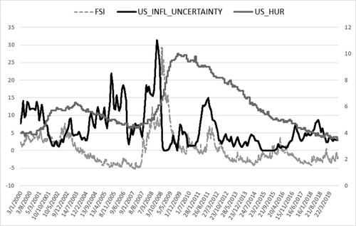
GSCI and HUR are log-transformed⁴ and together with the BAA_AAA spread level, the financial stress index volatility, and the inflation uncertainty, they are all five included in the realized variance model, where they are shown to be jointly significant. Due to the GARCH positivity constraints, we impose the positive sign restrictions on the estimated coefficients of the non-negative regressors. Therefore, our macro-financial linkages analysis is conducted on factors that exacerbate volatility. Figures 1–4 show the co-movement of DJ volatility with the macro-proxies. Rising economic policy uncertainty, default spreads, financial stress risk, commodity prices, unemployment, and inflation uncertainty, all lead to higher volatility levels, a characteristic feature of weaker economic stance.

Figure 1. DJ implied variance, DJ squared returns, and US EPU.

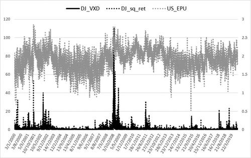
Figure 2. DJ realized variance, US EPU, and Moody’s default spread.

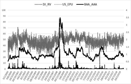
Figure 3. DJ realized variance, US EPU, and S&P GSCI index.

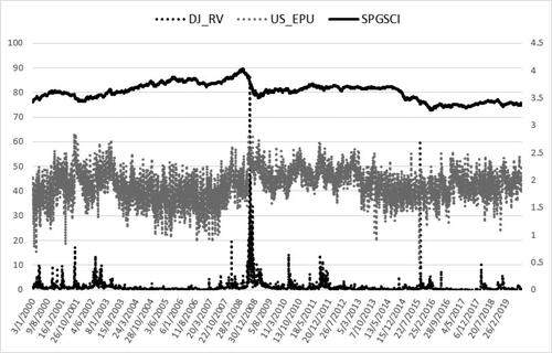
Figure 4. Global FSI, US unemployment rate, and US inflation uncertainty.

Before selecting the five macro-financial regressors for the realized variance equation, we tested a plethora of real activity, monetary, and financial candidates in daily and monthly frequency as discussed in the relevant literature. We chose the combination of jointly significant variables that minimize the information criteria and maximize the log-Likelihood score. Given the GARCH positivity constraints, we had to first exclude the variables with negative values and the variables with a negative impact on volatility. For example, the monthly IP growth rate and the daily term spread, the most representative activity indices, were significant when included alone and not with other macro-indices, they were estimated with negative signed coefficients and their time series come up with negative and non-negative values. Thus, we replaced them with a similar activity proxy, the unemployment rate, to reliably capture the business cycle phase. Among the daily variables tested with a significant positive effect but not jointly significant with other proxies or not complying with the positivity conditions are the 3-month-Libor rates, the 3-month-Treasury bill yields, the OFR FSI level, the crude oil futures implied volatility (OVX), and the Geopolitical Risk index by Caldara and Iacoviello (2018). We also excluded confidence or sentiment variables with a negative impact on volatility (e.g. the monthly Business and Consumer Confidence indices from the OECD database and the daily News Sentiment Index from the FRB San Francisco dataset, Buckman et al., 2020) but replaced them with the EPU positive effect. Overall, we resulted in a set of five macro-financial factors and the EPU impact, all exacerbating equities volatility. The six in total inflating macro-effects on the daily volatility pattern capture all major aspects of the business and financial cycle daily and monthly dynamics, keeping the simple AIM-HEAVY structure based on the GJR-GARCH-X and without allowing for any discount in the model’s reliability due to the positivity constraints imposed.

4. In-sample estimation results

Following Engle (2002) who introduced the GARCH-X process adding exogenous regressors in the conditional variance, various studies analyzed the asymptotic properties of this model considering a fractionally integrated covariate (see, for example, Francq & Thieu, 2019, for the univariate case, and Ling & McAleer, 2003; Han, 2015; Han & Kristensen, 2014; Nakatani and Teräsvirta, 2009; Pedersen, 2017, for the multivariate GARCH processes). For the asymmetric HEAVY extensions, we use the Gaussian QMLE and multistep-ahead predictors of the GJR-GARCH specification (Glosten et al., 1993). In line with Pedersen and Rahbek (2019), we first test for conditional heteroscedasticity (the arch effect) and since the homoscedasticity hypothesis is rejected, we perform one-sided significance tests on the regressors of the GARCH equations.

4.1. Benchmark and asymmetric formulation

We initially present the results of the benchmark model (Shephard & Sheppard, 2010), that is, the bivariate returns-realized measure system without asymmetries (Table 2). The preferred returns equation is a GARCH(1, 0)-X process without the lagged squared returns. The own Arch effect, α_rr, becomes insignificant when we include the lagged realized measure cross effect, α_rR. For the SSR realized variance, we choose a GARCH(1, 1) without the returns impact. The chosen benchmark HEAVY specifications, after testing all three alternative GARCH models of order (1, 1), (1, 1)-X and (1, 0)-X, are identical to Shephard and Sheppard (2010) with similar coefficients values and the same finding that the intra-daily realized measure does all the work at moving around both conditional variances. The benchmark’s finding, as we demonstrate hereafter, does not apply for the extended asymmetric system. Finally, the Sign Bias test (SBT) of Engle and Ng (1993) shows that the returns asymmetric effect is ignored by the benchmark estimations (p-values < 0.05).

Table 2. The bivariate benchmark HEAVY system (eq. (3)(3) $$\begin{array}{c}\text{HEAVY}-r\text{:}\mathrm{ }(1-{\beta }_{r}L){\sigma }_{rt}^2={\omega }_r+{\alpha }_{rR}L(R{M}_t),\\ \text{HEAVY}-R\text{:}\mathrm{ }(1-{\beta }_{R}L){\sigma }_{Rt}^2={\omega }_R+{\alpha }_{RR}L(R{M}_t).\end{array}$$(3) ).

	DJ	SP	EU	FTSE	DAX	CAC	AEX
Panel A. $\text{HEAVY}-\mathrm{r}:$ $(1-{\beta }_{r}L){\sigma }_{rt}^2={\omega }_r+{\alpha }_{rR}L(R{M}_t)$
βr	$\underset{{(16.08)}^{\ast \ast \ast }}{0.65}$	$\underset{{(12.35)}^{\ast \ast \ast }}{0.62}$	$\underset{{(14.28)}^{\ast \ast \ast }}{0.64}$	$\underset{{(14.09)}^{\ast \ast \ast }}{0.64}$	$\underset{{(13.01)}^{\ast \ast \ast }}{0.63}$	$\underset{{(7.46)}^{\ast \ast \ast }}{0.43}$	$\underset{{(9.59)}^{\ast \ast \ast }}{0.53}$
αrR	$\underset{{(7.66)}^{\ast \ast \ast }}{0.39}$	$\underset{{(6.98)}^{\ast \ast \ast }}{0.49}$	$\underset{{(7.62)}^{\ast \ast \ast }}{0.45}$	$\underset{{(7.21)}^{\ast \ast \ast }}{0.38}$	$\underset{{(7.23)}^{\ast \ast \ast }}{0.47}$	$\underset{{(8.99)}^{\ast \ast \ast }}{0.83}$	$\underset{{(8.29)}^{\ast \ast \ast }}{0.76}$
SBT	$\underset{[0.00]}{3.07}$	$\underset{[0.01]}{2.58}$	$\underset{[0.00]}{3.47}$	$\underset{[0.01]}{2.65}$	$\underset{[0.00]}{4.08}$	$\underset{[0.05]}{1.93}$	$\underset{[0.02]}{2.35}$
AIC	2.5613	2.6337	3.0891	2.6391	3.1362	3.0575	$2.9082$
lnL	$-6335.04$	$-6520.63$	$-7376.85$	$-6146.20$	$-7451.64$	$-7307.48$	$-6950.61$
Panel B. $\text{HEAVY}-\mathrm{R}:$ $(1-{\beta }_{R}L){\sigma }_{Rt}^2={\omega }_R+{\alpha }_{RR}L(R{M}_t)$
βR	$\underset{{(14.06)}^{\ast \ast \ast }}{0.57}$	$\underset{{(13.77)}^{\ast \ast \ast }}{0.52}$	$\underset{{(16.38)}^{\ast \ast \ast }}{0.58}$	$\underset{{(16.28)}^{\ast \ast \ast }}{0.62}$	$\underset{{(19.53)}^{\ast \ast \ast }}{0.59}$	$\underset{{(16.26)}^{\ast \ast \ast }}{0.56}$	$\underset{{(16.19)}^{\ast \ast \ast }}{0.54}$
αRR	$\underset{{(9.26)}^{\ast \ast \ast }}{0.44}$	$\underset{{(11.26)}^{\ast \ast \ast }}{0.48}$	$\underset{{(11.50)}^{\ast \ast \ast }}{0.40}$	$\underset{{(9.12)}^{\ast \ast \ast }}{0.37}$	$\underset{{(13.28)}^{\ast \ast \ast }}{0.40}$	$\underset{{(12.12)}^{\ast \ast \ast }}{0.42}$	$\underset{{(12.85)}^{\ast \ast \ast }}{0.44}$
SBT	$\underset{[0.00]}{3.68}$	$\underset{[0.00]}{4.74}$	$\underset{[0.01]}{2.61}$	$\underset{[0.01]}{2.64}$	$\underset{[0.01]}{2.83}$	$\underset{[0.05]}{1.98}$	$\underset{[0.00]}{2.94}$
AIC	2.3978	2.3511	2.8544	2.5475	2.8201	2.6802	$2.4764$
lnL	$-5930.31$	$-5820.68$	$-6816.20$	$-5932.64$	$-6700.30$	$-6405.42$	$-5918.14$

Notes: The numbers in parentheses are t-statistics. The numbers in square brackets are p-values. ${}^{\ast \ast \ast },$${}^{\ast \ast },$ ${}^{\ast }$ denote significance at the 0.01, 0.05, 0.10 level, respectively. SBT stands for the Sign Bias test of Engle and Ng (1993).

AIC is the Akaike Information Criterion value and lnL the log-likelihood value for each specification.

Next, we enrich the bivariate benchmark specification with asymmetries. Our first extension, the Asymmetric HEAVY model (eq. (4)(4) $$(1-{\beta }_{i}L){\sigma }_{it}^2={\omega }_i+({\alpha }_{ir}+{\gamma }_{ir}{s}_{t-1})L(r_t^2)+({\alpha }_{iR}+{\gamma }_{iR}{s}_{t-1})L(R{M}_t),\text{\hspace{0.5em}for\hspace{0.5em}}i=r,R,$$(4) ), involves again the two volatility measures proposed by Shephard and Sheppard (2010), the conditional variance of returns and the realized variance. Table 2 presents the in-sample results across the seven indices. The SBT values show that asymmetries are not omitted anymore, while the information criteria and log-likelihood scores clearly prefer the asymmetric formulation. Our main finding here, in the presence of leverage, is the bidirectional spillover effect between the two volatility series, whereas in the benchmark model the realized measure does not receive any effect from daily squared returns. We estimate significant leverage parameters with double asymmetries incorporated in both equations. The returns conditional variance is affected by own asymmetries (γ_rr), the realized variance (α_rR), and cross asymmetries (γ_rR). The realized measure trajectory is determined by the own Heavy terms (lagged realized variance, α_RR, and own asymmetry, γ_RR) with the exception of FTSE where own asymmetry is insignificant and excluded. Moreover, we estimate significant cross Arch asymmetry impact, γ_Rr, but without the Arch term (α_Rr).

4.2. The implied variance extension

After illustrating the significant contribution of asymmetries in the benchmark model, we proceed with the second HEAVY extension. In light of the ample evidence in favor of implied variance as an additional useful source of information for volatility forecasting, we initially include IVs in two asymmetric bivariate systems: the first is a combination of IV with returns and the second involves IV with realized variance (Tables 4 and 5). Comparing the returns equations in Tables 3 and 4, the conditional variance of returns shows a better fit when the realized variance is included for four out of the seven indices (SP, DAX, CAC, AEX), while in the remaining three cases (DJ, EU, FTSE) the implied variance is the preferred regressor in the returns GJR-GARCH(1,0)-X specification with both asymmetric effects from returns and IVs. Interestingly, the own leverage terms (γ_rr) are higher in the returns-IV system across all indices. In the realized variance specifications of Tables 3 and 5, we observe that realized variance is better modeled with the direct IV contribution but without IV cross asymmetry compared to the A-HEAVY-R equation with the effect from lagged negative squared returns. When we include IV in the realized measure equation, we estimate significantly lower Garch effects (β_R) and higher own Heavy asymmetries (γ_RR). Hence, we can assert that in realized measure modeling when IV information is incorporated, the effects from its own lagged conditional mean is limited. Simultaneously, the own leverage contribution is stronger in all cases, even in FTSE where γ_RR is excluded in the Asymmetric bivariate model without IVs. Assessing the IV equation results of the two bivariate systems (Tables 4 and 5), we demonstrate that the best model for IV per se in most indices is the GARCH(1,1)-X with the cross asymmetry of returns (γ_Ir) as regressor and without own leverage term significant (γ_II). Only for EU, we statistically prefer the GARCH(1,1) specification without any covariate (both Heavy and Arch effects are insignificant and therefore excluded).

Table 3. The bivariate A-HEAVY system (eq. (4)(4) $$(1-{\beta }_{i}L){\sigma }_{it}^2={\omega }_i+({\alpha }_{ir}+{\gamma }_{ir}{s}_{t-1})L(r_t^2)+({\alpha }_{iR}+{\gamma }_{iR}{s}_{t-1})L(R{M}_t),\text{\hspace{0.5em}for\hspace{0.5em}}i=r,R,$$(4) ).

	DJ	SP	EU	FTSE	DAX	CAC	AEX
Panel A. A-$\text{HEAVY}-\mathrm{r}$ $\begin{array}{c}(1-{\beta }_{r}L){\sigma }_{rt}^2={\omega }_r+({\alpha }_{rr}+{\gamma }_{rr}{s}_{t-1})L(r_t^2)+({\alpha }_{rR}+{\gamma }_{rR}{s}_{t-1})L(R{M}_t)\end{array}$
βr	$\underset{{(32.67)}^{\ast \ast \ast }}{0.76}$	$\underset{{(26.50)}^{\ast \ast \ast }}{0.73}$	$\underset{{(19.42)}^{\ast \ast \ast }}{0.77}$	$\underset{{(30.30)}^{\ast \ast \ast }}{0.80}$	$\underset{{(17.77)}^{\ast \ast \ast }}{0.74}$	$\underset{{(5.85)}^{\ast \ast \ast }}{0.57}$	$\underset{{(13.56)}^{\ast \ast \ast }}{0.71}$
γrr	$\underset{{(3.59)}^{\ast \ast \ast }}{0.08}$	$\underset{{(1.66)}^{\ast }}{0.04}$	$\underset{{(3.38)}^{\ast \ast \ast }}{0.08}$	$\underset{{(5.73)}^{\ast \ast \ast }}{0.11}$	$\underset{{(2.79)}^{\ast \ast \ast }}{0.06}$	$\underset{{(2.14)}^{\ast \ast }}{0.07}$	$\underset{{(3.97)}^{\ast \ast \ast }}{0.10}$
αrR	$\underset{{(3.44)}^{\ast \ast \ast }}{0.11}$	$\underset{{(3.86)}^{\ast \ast \ast }}{0.16}$	$\underset{{(1.97)}^{\ast \ast }}{0.13}$	$\underset{{(1.90)}^{\ast }}{0.05}$	$\underset{{(2.60)}^{\ast \ast \ast }}{0.17}$	$\underset{{(2.32)}^{\ast \ast }}{0.43}$	$\underset{{(2.55)}^{\ast \ast \ast }}{0.24}$
γrR	$\underset{{(5.09)}^{\ast \ast \ast }}{0.22}$	$\underset{{(5.96)}^{\ast \ast \ast }}{0.32}$	$\underset{{(3.56)}^{\ast \ast \ast }}{0.20}$	$\underset{{(4.38)}^{\ast \ast \ast }}{0.16}$	$\underset{{(3.60)}^{\ast \ast \ast }}{0.20}$	$\underset{{(3.49)}^{\ast \ast \ast }}{0.27}$	$\underset{{(4.24)}^{\ast \ast \ast }}{0.25}$
SBT	$\underset{[0.75]}{0.32}$	$\underset{[0.73]}{0.35}$	$\underset{[0.45]}{0.75}$	$\underset{[0.33]}{0.98}$	$\underset{[0.30]}{1.04}$	$\underset{[0.76]}{0.31}$	$\underset{[0.40]}{0.85}$
AIC	2.5407	2.6150	3.0748	2.6109	3.1261	3.0497	2.8946
lnL	$-6280.59$	$-6470.95$	$-7339.14$	$-6077.03$	$-7424.27$	$-7285.21$	$-6914.64$
Panel B. A-$\text{HEAVY}-\mathrm{R}$ $\begin{array}{c}(1-{\beta }_{R}L){\sigma }_{Rt}^2={\omega }_R+({\alpha }_{RR}+{\gamma }_{RR}{s}_{t-1})L(R{M}_t)+({\alpha }_{Rr}+{\gamma }_{Rr}{s}_{t-1})L(r_t^2)\end{array}$
βR	$\underset{{(27.63)}^{\ast \ast \ast }}{0.67}$	$\underset{{(23.65)}^{\ast \ast \ast }}{0.64}$	$\underset{{(20.59)}^{\ast \ast \ast }}{0.69}$	$\underset{{(27.48)}^{\ast \ast \ast }}{0.73}$	$\underset{{(26.36)}^{\ast \ast \ast }}{0.70}$	$\underset{{(20.09)}^{\ast \ast \ast }}{0.68}$	$\underset{{(18.06)}^{\ast \ast \ast }}{0.64}$
αRR	$\underset{{(8.63)}^{\ast \ast \ast }}{0.20}$	$\underset{{(9.17)}^{\ast \ast \ast }}{0.24}$	$\underset{{(4.51)}^{\ast \ast \ast }}{0.20}$	$\underset{{(5.98)}^{\ast \ast \ast }}{0.19}$	$\underset{{(7.93)}^{\ast \ast \ast }}{0.21}$	$\underset{{(6.84)}^{\ast \ast \ast }}{0.22}$	$\underset{{(6.25)}^{\ast \ast \ast }}{0.25}$
γRR	$\underset{{(5.64)}^{\ast \ast \ast }}{0.12}$	$\underset{{(5.77)}^{\ast \ast \ast }}{0.12}$	$\underset{{(1.69)}^{\ast }}{0.05}$		$\underset{{(4.11)}^{\ast \ast \ast }}{0.07}$	$\underset{{(3.47)}^{\ast \ast \ast }}{0.06}$	$\underset{{(2.36)}^{\ast \ast \ast }}{0.05}$
γRr	$\underset{{(5.25)}^{\ast \ast \ast }}{0.09}$	$\underset{{(6.31)}^{\ast \ast \ast }}{0.08}$	$\underset{{(9.40)}^{\ast \ast \ast }}{0.09}$	$\underset{{(9.19)}^{\ast \ast \ast }}{0.12}$	$\underset{{(8.66)}^{\ast \ast \ast }}{0.06}$	$\underset{{(8.45)}^{\ast \ast \ast }}{0.06}$	$\underset{{(8.59)}^{\ast \ast \ast }}{0.07}$
SBT	$\underset{[0.23]}{1.21}$	$\underset{[0.28]}{1.07}$	$\underset{[0.18]}{1.33}$	$\underset{[0.13]}{1.52}$	$\underset{[0.55]}{0.60}$	$\underset{[0.68]}{0.41}$	$\underset{[0.64]}{0.46}$
AIC	2.3825	2.3386	2.8446	2.5337	2.8127	2.6727	2.4671
lnL	$-5889.36$	$-5786.46$	$-6789.22$	$-5898.23$	$-6679.42$	$-6384.16$	$-5892.59$

Notes: See notes in Table 2.

Table 4. The bivariate asymmetric returns-implied variance system.

	DJ	SP	EU	FTSE	DAX	CAC	AEX
Panel A. Returns $\begin{array}{c}(1-{\beta }_{r}L){\sigma }_{rt}^2={\omega }_r+({\alpha }_{rr}+{\gamma }_{rr}{s}_{t-1})L(r_t^2)+({\alpha }_{rI}+{\gamma }_{rI}{s}_{t-1})L(I{V}_t)\end{array}$
βr	$\underset{{(20.23)}^{\ast \ast \ast }}{0.74}$	$\underset{{(15.03)}^{\ast \ast \ast }}{0.72}$	$\underset{{(17.75)}^{\ast \ast \ast }}{0.74}$	$\underset{{(21.36)}^{\ast \ast \ast }}{0.76}$	$\underset{{(16.96)}^{\ast \ast \ast }}{0.74}$	$\underset{{(16.40)}^{\ast \ast \ast }}{0.73}$	$\underset{{(29.26)}^{\ast \ast \ast }}{0.77}$
γrr	$\underset{{(7.44)}^{\ast \ast \ast }}{0.15}$	$\underset{{(5.85)}^{\ast \ast \ast }}{0.13}$	$\underset{{(6.82)}^{\ast \ast \ast }}{0.15}$	$\underset{{(8.07)}^{\ast \ast \ast }}{0.17}$	$\underset{{(7.05)}^{\ast \ast \ast }}{0.14}$	$\underset{{(7.35)}^{\ast \ast \ast }}{0.16}$	$\underset{{(8.32)}^{\ast \ast \ast }}{0.16}$
αrI	$\underset{{(2.56)}^{\ast \ast \ast }}{0.08}$	$\underset{{(2.18)}^{\ast \ast }}{0.08}$	$\underset{{(2.24)}^{\ast \ast }}{0.08}$	$\underset{{(2.49)}^{\ast \ast \ast }}{0.06}$	$\underset{{(2.66)}^{\ast \ast \ast }}{0.10}$	$\underset{{(2.15)}^{\ast \ast }}{0.09}$	$\underset{{(2.47)}^{\ast \ast \ast }}{0.05}$
γrI	$\underset{{(4.70)}^{\ast \ast \ast }}{0.12}$	$\underset{{(5.44)}^{\ast \ast \ast }}{0.15}$	$\underset{{(4.63)}^{\ast \ast \ast }}{0.12}$	$\underset{{(3.78)}^{\ast \ast \ast }}{0.08}$	$\underset{{(3.85)}^{\ast \ast \ast }}{0.11}$	$\underset{{(4.69)}^{\ast \ast \ast }}{0.14}$	$\underset{{(5.40)}^{\ast \ast \ast }}{0.11}$
AIC	2.5386	2.6182	3.0672	2.6032	3.1302	3.0527	2.8958
lnL	$-6275.37$	$-6478.89$	$-7321.00$	$-6059.07$	$-7433.87$	$-7292.42$	$-6917.44$
Panel B. Implied Variance $\begin{array}{c}(1-{\beta }_{I}L){\sigma }_{It}^2={\omega }_I+({\alpha }_{II}+{\gamma }_{II}{s}_{t-1})L(I{V}_t)+({\alpha }_{Ir}+{\gamma }_{Ir}{s}_{t-1})L(r_t^2)\end{array}$
βI	$\underset{{(5.28)}^{\ast \ast \ast }}{0.15}$	$\underset{{(5.08)}^{\ast \ast \ast }}{0.29}$	$\underset{{(3.01)}^{\ast \ast \ast }}{0.39}$	$\underset{{(8.87)}^{\ast \ast \ast }}{0.38}$	$\underset{{(3.24)}^{\ast \ast \ast }}{0.24}$	$\underset{{(5.15)}^{\ast \ast \ast }}{0.35}$	$\underset{{(14.51)}^{\ast \ast \ast }}{0.47}$
αII	$\underset{{(29.66)}^{\ast \ast \ast }}{0.84}$	$\underset{{(11.55)}^{\ast \ast \ast }}{0.69}$	$\underset{{(6.81)}^{\ast \ast \ast }}{0.60}$	$\underset{{(13.72)}^{\ast \ast \ast }}{0.60}$	$\underset{{(9.57)}^{\ast \ast \ast }}{0.74}$	$\underset{{(8.95)}^{\ast \ast \ast }}{0.62}$	$\underset{{(15.16)}^{\ast \ast \ast }}{0.50}$
γIr	$\underset{{(2.55)}^{\ast \ast \ast }}{0.01}$	$\underset{{(2.99)}^{\ast \ast \ast }}{0.03}$	$\underset{{(3.85)}^{\ast \ast \ast }}{0.03}$	$\underset{{(7.42)}^{\ast \ast \ast }}{0.04}$	$\underset{{(3.48)}^{\ast \ast \ast }}{0.02}$	$\underset{{(6.30)}^{\ast \ast \ast }}{0.04}$	$\underset{{(11.05)}^{\ast \ast \ast }}{0.05}$
AIC	3.0120	3.1191	3.4958	3.0477	3.4640	3.3757	3.3164
lnL	$-7447.59$	$-7720.53$	$-8345.74$	$-7095.53$	$-8228.13$	$-8065.66$	$-7923.75$

Notes: See notes in Table 2.

Table 5. The bivariate asymmetric realized measure-implied variance system.

	DJ	SP	EU	FTSE	DAX	CAC	AEX
Panel A. Realized Variance $\begin{array}{c}(1-{\beta }_{R}L){\sigma }_{Rt}^2={\omega }_R+({\alpha }_{RR}+{\gamma }_{RR}{s}_{t-1})L(R{M}_t)+({\alpha }_{RI}+{\gamma }_{RI}{s}_{t-1})L(I{V}_t)\end{array}$
βR	$\underset{{(9.25)}^{\ast \ast \ast }}{0.47}$	$\underset{{(7.33)}^{\ast \ast \ast }}{0.36}$	$\underset{{(5.16)}^{\ast \ast \ast }}{0.38}$	$\underset{{(4.90)}^{\ast \ast \ast }}{0.37}$	$\underset{{(7.39)}^{\ast \ast \ast }}{0.46}$	$\underset{{(8.18)}^{\ast \ast \ast }}{0.42}$	$\underset{{(7.60)}^{\ast \ast \ast }}{0.41}$
αRR	$\underset{{(7.89)}^{\ast \ast \ast }}{0.21}$	$\underset{{(9.19)}^{\ast \ast \ast }}{0.26}$	$\underset{{(5.27)}^{\ast \ast \ast }}{0.20}$	$\underset{{(4.50)}^{\ast \ast \ast }}{0.15}$	$\underset{{(7.71)}^{\ast \ast \ast }}{0.23}$	$\underset{{(8.51)}^{\ast \ast \ast }}{0.26}$	$\underset{{(8.27)}^{\ast \ast \ast }}{0.27}$
γRR	$\underset{{(8.49)}^{\ast \ast \ast }}{0.26}$	$\underset{{(9.16)}^{\ast \ast \ast }}{0.23}$	$\underset{{(5.83)}^{\ast \ast \ast }}{0.18}$	$\underset{{(5.28)}^{\ast \ast \ast }}{0.19}$	$\underset{{(8.39)}^{\ast \ast \ast }}{0.16}$	$\underset{{(8.88)}^{\ast \ast \ast }}{0.17}$	$\underset{{(8.89)}^{\ast \ast \ast }}{0.18}$
αRI	$\underset{{(5.34)}^{\ast \ast \ast }}{0.14}$	$\underset{{(6.75)}^{\ast \ast \ast }}{0.17}$	$\underset{{(4.99)}^{\ast \ast \ast }}{0.19}$	$\underset{{(5.33)}^{\ast \ast \ast }}{0.25}$	$\underset{{(4.48)}^{\ast \ast \ast }}{0.14}$	$\underset{{(6.00)}^{\ast \ast \ast }}{0.13}$	$\underset{{(5.75)}^{\ast \ast \ast }}{0.10}$
AIC	2.3795	2.3316	2.8392	2.5276	2.8108	2.6709	2.4664
lnL	$-5883.09$	$-5770.45$	$-6777.73$	$-5884.24$	$-6676.26$	$-6381.03$	$-5892.07$
Panel B. Implied Variance $\begin{array}{c}(1-{\beta }_{I}L){\sigma }_{It}^2={\omega }_I+({\alpha }_{II}+{\gamma }_{II}{s}_{t-1})L(I{V}_t)+({\alpha }_{IR}+{\gamma }_{IR}{s}_{t-1})L(R{M}_t)\end{array}$
βI	$\underset{{(5.47)}^{\ast \ast \ast }}{0.14}$	$\underset{{(5.03)}^{\ast \ast \ast }}{0.28}$	$\underset{{(3.81)}^{\ast \ast \ast }}{0.38}$	$\underset{{(8.19)}^{\ast \ast \ast }}{0.35}$	$\underset{{(3.10)}^{\ast \ast \ast }}{0.22}$	$\underset{{(5.19)}^{\ast \ast \ast }}{0.32}$	$\underset{{(13.78)}^{\ast \ast \ast }}{0.44}$
αII	$\underset{{(31.83)}^{\ast \ast \ast }}{0.84}$	$\underset{{(11.97)}^{\ast \ast \ast }}{0.69}$	$\underset{{(6.26)}^{\ast \ast \ast }}{0.61}$	$\underset{{(14.38)}^{\ast \ast \ast }}{0.63}$	$\underset{{(9.99)}^{\ast \ast \ast }}{0.75}$	$\underset{{(9.90)}^{\ast \ast \ast }}{0.64}$	$\underset{{(15.85)}^{\ast \ast \ast }}{0.53}$
γIR	$\underset{{(2.56)}^{\ast \ast \ast }}{0.02}$	$\underset{{(3.52)}^{\ast \ast \ast }}{0.05}$		$\underset{{(4.23)}^{\ast \ast \ast }}{0.04}$	$\underset{{(2.85)}^{\ast \ast \ast }}{0.03}$	$\underset{{(5.98)}^{\ast \ast \ast }}{0.07}$	$\underset{{(8.39)}^{\ast \ast \ast }}{0.08}$
AIC	3.0120	3.1191	3.4955	3.0479	3.4641	3.3758	3.3167
lnL	$-7447.58$	$-7720.55$	$-8347.76$	$-7096.17$	$-8228.32$	$-8065.95$	$-7924.66$

Notes: See notes in Table 2.

Next, we estimate the trivariate system with all three financial volatilities, namely the Asymmetric-Implied HEAVY (Table 6). Both conditional variances of returns and SSR realized variance receive the options market information content. The returns results (Panel A) show that both intra-daily (RM) and options-implied sources are informative for the conditional variance of daily returns, with own asymmetries (γ_rr) always significant and cross asymmetries either from IVs or RMs. Only the DJ specification includes all three Arch, Heavy, and Implied asymmetries. The realized variance estimations (Panel B) involve the negative squared returns and the IV apart from the own RM leverage. Overall, the trivariate specification for returns and RM outperforms in-sample all bivariate models (Tables 2–5) confirming the significant information role of options-inferred variance in accordance with the extant literature. On the basis of this evidence, we conjecture that daily and intra-daily volatility modeling should undoubtedly utilize the ex-ante market forecast for future volatility besides asymmetries. Regarding the IV per se (Panel C), after trying all trivariate combinations, we statistically prefer a univariate GARCH(1,1) specification for the US indices and two European markets, EU and DAX, whereas SSR IVs of FTSE, CAC, and AEX are best estimated with the cross Arch leverage effect.

Table 6. The trivariate AI-HEAVY system.

	DJ	SP	EU	FTSE	DAX	CAC	AEX
Panel A. AI-$\text{HEAVY}-\mathrm{r}$ $\begin{array}{c}(1-{\beta }_{r}L){\sigma }_{rt}^2={\omega }_r+({\alpha }_{rr}+{\gamma }_{rr}{s}_{t-1})L(r_t^2)+\\ ({\alpha }_{rR}+{\gamma }_{rR}{s}_{t-1})L(R{M}_t)+({\alpha }_{rI}+{\gamma }_{rI}{s}_{t-1})L(I{V}_t)\end{array}$
βr	$\underset{{(15.93)}^{\ast \ast \ast }}{0.69}$	$\underset{{(20.92)}^{\ast \ast \ast }}{0.70}$	$\underset{{(14.17)}^{\ast \ast \ast }}{0.69}$	$\underset{{(18.51)}^{\ast \ast \ast }}{0.72}$	$\underset{{(11.49)}^{\ast \ast \ast }}{0.68}$	$\underset{{(3.93)}^{\ast \ast \ast }}{0.45}$	$\underset{{(7.51)}^{\ast \ast \ast }}{0.61}$
γrr	$\underset{{(3.44)}^{\ast \ast \ast }}{0.09}$	$\underset{{(1.84)}^{\ast }}{0.05}$	$\underset{{(2.63)}^{\ast \ast \ast }}{0.08}$	$\underset{{(5.29)}^{\ast \ast \ast }}{0.13}$	$\underset{{(2.29)}^{\ast \ast }}{0.06}$	$\underset{{(2.22)}^{\ast \ast }}{0.06}$	$\underset{{(3.28)}^{\ast \ast \ast }}{0.10}$
αrR	$\underset{{(1.78)}^{\ast }}{0.07}$	$\underset{{(4.86)}^{\ast \ast \ast }}{0.22}$			$\underset{{(1.67)}^{\ast }}{0.09}$	$\underset{{(3.62)}^{\ast \ast \ast }}{0.45}$	$\underset{{(1.78)}^{\ast }}{0.17}$
γrR	$\underset{{(2.26)}^{\ast \ast }}{0.16}$		$\underset{{(5.48)}^{\ast \ast \ast }}{0.28}$	$\underset{{(4.48)}^{\ast \ast \ast }}{0.16}$	$\underset{{(4.87)}^{\ast \ast \ast }}{0.25}$		$\underset{{(4.95)}^{\ast \ast \ast }}{0.30}$
αrI	$\underset{{(2.35)}^{\ast \ast }}{0.08}$		$\underset{{(3.11)}^{\ast \ast \ast }}{0.12}$	$\underset{{(3.69)}^{\ast \ast \ast }}{0.09}$	$\underset{{(2.40)}^{\ast \ast }}{0.10}$	$\underset{{(1.75)}^{\ast }}{0.12}$	$\underset{{(2.91)}^{\ast \ast \ast }}{0.11}$
γrI	$\underset{{(1.76)}^{\ast }}{0.06}$	$\underset{{(6.63)}^{\ast \ast \ast }}{0.16}$				$\underset{{(3.68)}^{\ast \ast \ast }}{0.14}$
AIC	2.5292	2.6060	3.0606	2.6000	3.1204	3.0396	2.8863
lnL	$-6250.34$	$-6448.83$	$-7305.23$	$-6051.77$	$-7409.73$	$-7260.22$	$-6893.75$
Panel B. AI-$\text{HEAVY}-\mathrm{R}$ $\begin{array}{c}(1-{\beta }_{R}L){\sigma }_{Rt}^2={\omega }_R+({\alpha }_{RR}+{\gamma }_{RR}{s}_{t-1})L(R{M}_t)+\\ ({\alpha }_{Rr}+{\gamma }_{Rr}{s}_{t-1})L(r_t^2)+({\alpha }_{RI}+{\gamma }_{RI}{s}_{t-1})L(I{V}_t)\end{array}$
βR	$\underset{{(15.18)}^{\ast \ast \ast }}{0.55}$	$\underset{{(11.65)}^{\ast \ast \ast }}{0.46}$	$\underset{{(8.34)}^{\ast \ast \ast }}{0.51}$	$\underset{{(7.19)}^{\ast \ast \ast }}{0.55}$	$\underset{{(11.23)}^{\ast \ast \ast }}{0.56}$	$\underset{{(11.05)}^{\ast \ast \ast }}{0.52}$	$\underset{{(9.88)}^{\ast \ast \ast }}{0.49}$
αRR	$\underset{{(7.70)}^{\ast \ast \ast }}{0.16}$	$\underset{{(8.08)}^{\ast \ast \ast }}{0.20}$	$\underset{{(4.42)}^{\ast \ast \ast }}{0.14}$	$\underset{{(3.14)}^{\ast \ast \ast }}{0.10}$	$\underset{{(7.20)}^{\ast \ast \ast }}{0.19}$	$\underset{{(7.04)}^{\ast \ast \ast }}{0.20}$	$\underset{{(7.16)}^{\ast \ast \ast }}{0.22}$
γRR	$\underset{{(5.44)}^{\ast \ast \ast }}{0.15}$	$\underset{{(5.46)}^{\ast \ast \ast }}{0.13}$	$\underset{{(2.87)}^{\ast \ast \ast }}{0.08}$	$\underset{{(2.04)}^{\ast \ast }}{0.06}$	$\underset{{(4.62)}^{\ast \ast \ast }}{0.08}$	$\underset{{(4.28)}^{\ast \ast \ast }}{0.08}$	$\underset{{(3.36)}^{\ast \ast \ast }}{0.07}$
γRr	$\underset{{(5.84)}^{\ast \ast \ast }}{0.11}$	$\underset{{(5.99)}^{\ast \ast \ast }}{0.09}$	$\underset{{(8.19)}^{\ast \ast \ast }}{0.10}$	$\underset{{(7.74)}^{\ast \ast \ast }}{0.12}$	$\underset{{(7.84)}^{\ast \ast \ast }}{0.07}$	$\underset{{(7.93)}^{\ast \ast \ast }}{0.07}$	$\underset{{(8.58)}^{\ast \ast \ast }}{0.08}$
αRI	$\underset{{(5.06)}^{\ast \ast \ast }}{0.11}$	$\underset{{(6.94)}^{\ast \ast \ast }}{0.13}$	$\underset{{(4.56)}^{\ast \ast \ast }}{0.14}$	$\underset{{(3.68)}^{\ast \ast \ast }}{0.16}$	$\underset{{(4.66)}^{\ast \ast \ast }}{0.10}$	$\underset{{(5.84)}^{\ast \ast \ast }}{0.10}$	$\underset{{(5.52)}^{\ast \ast \ast }}{0.08}$
AIC	2.3743	2.3277	2.8352	2.5226	2.8080	2.6674	2.4616
lnL	$-5868.10$	$-5758.51$	$-6765.77$	$-5870.40$	$-6667.25$	$-6370.45$	$-5878.44$
Panel C. AI-$\text{HEAVY}-\mathrm{I}$ $\begin{array}{c}(1-{\beta }_{I}L){\sigma }_{It}^2={\omega }_I+({\alpha }_{II}+{\gamma }_{II}{s}_{t-1})L(I{V}_t)+\\ ({\alpha }_{IR}+{\gamma }_{IR}{s}_{t-1})L(R{M}_t)+({\alpha }_{Ir}+{\gamma }_{Ir}{s}_{t-1})L(r_t^2)\end{array}$
βI	$\underset{{(4.64)}^{\ast \ast \ast }}{0.11}$	$\underset{{(4.76)}^{\ast \ast \ast }}{0.26}$	$\underset{{(3.81)}^{\ast \ast \ast }}{0.38}$	$\underset{{(8.87)}^{\ast \ast \ast }}{0.38}$	$\underset{{(3.05)}^{\ast \ast \ast }}{0.20}$	$\underset{{(5.15)}^{\ast \ast \ast }}{0.35}$	$\underset{{(14.51)}^{\ast \ast \ast }}{0.47}$
αII	$\underset{{(36.57)}^{\ast \ast \ast }}{0.88}$	$\underset{{(13.77)}^{\ast \ast \ast }}{0.73}$	$\underset{{(6.26)}^{\ast \ast \ast }}{0.61}$	$\underset{{(13.72)}^{\ast \ast \ast }}{0.60}$	$\underset{{(11.82)}^{\ast \ast \ast }}{0.79}$	$\underset{{(8.95)}^{\ast \ast \ast }}{0.62}$	$\underset{{(15.16)}^{\ast \ast \ast }}{0.50}$
γIr				$\underset{{(7.42)}^{\ast \ast \ast }}{0.04}$		$\underset{{(6.30)}^{\ast \ast \ast }}{0.04}$	$\underset{{(11.05)}^{\ast \ast \ast }}{0.05}$
AIC	3.0118	3.1190	3.4955	3.0477	3.4638	3.3757	3.3164
lnL	$-7449.60$	$-7722.89$	$-8347.76$	$-7095.53$	$-8230.38$	$-8065.66$	$-7923.75$

Notes: See notes in Table 2.

4.3. The AIM-HEAVY specification

Research on the uncertainty-volatility link in the high-frequency domain is in its infancy. Antonakakis et al. (2013) have estimated the time-varying correlations of S&P 500 returns, VIX, and EPU in a monthly context, resulting in a positive VIX-EPU and a negative returns-EPU average correlation, confirming Pastor and Veronesi (2013) monthly OLS results. Higher uncertainty weakens equities performance and coincides with elevated volatility. Moreover, a positive relation between monthly implied volatilities and macro-uncertainty, proxied by the disagreement on macro-fundamentals’ projections among economists, has been recently asserted by Li et al. (2020).

In the present study, we include the EPU index as the fourth dependent variable in a tetravariate system for volatility modeling. Alongside the three financial uncertainty measures, we investigate the macroeconomic information effects from US and UK to the US and the European stock markets, respectively. The tetravariate Asymmetric-Implied-Macro HEAVY model (Table 7) estimates four conditional variances: returns, SSR realized and implied variance, and SSR EPU. For the first two measures (Panels A & B), we obtain similar results to the trivariate model (Table 6, Panels A & B) with the addition of the EPU exacerbating impact on financial volatility. The EPU impact is either direct (α_rU) or asymmetric (${\varphi }_{rU}$), with asymmetry in macro-uncertainty defined as the positive EPU shock and not the negative shock as in the returns case. The inflating impact from increased US and UK EPU is in line with Pastor and Veronesi (2013), who first associated volatilities with EPU, concluding on a positive link. The positive link corroborates Conrad and Loch (2015), among others, on the consumer confidence negative effect. Confidence is the antipode of uncertainty. Consequently, we estimate here an opposite sign, as expected. We further observe, according to AIC and lnL scores, a better in-sample fit of returns and RM macro-models compared to trivariate equations without EPU regressors. The improvement coming from the macro-information content is small but significant. On the other hand, the IV specification is identical to the trivariate system (Tables 6 and 7, Panel C) given that EPU exerts no significant influence on option-inferred variability, and therefore we still prefer the univariate model or the specification with the lagged negative squared returns. Hence, we can deduce that the options-market volatility expectation may subsume the macroeconomic information included in the EPU metric. Intriguingly, the policy uncertainty (Table 7, Panel D) is best estimated with the positive asymmetry effect and receives no financial volatility impact from either of the three measures⁵.

Table 7. The tetravariate AIM-HEAVY system (eq. (6)(6) $$\begin{array}{c}(1-{\beta }_{i}L){\sigma }_{it}^2={\omega }_i+({\alpha }_{ir}+{\gamma }_{ir}{s}_{t-1})L(r_t^2)+({\alpha }_{iR}+{\gamma }_{iR}{s}_{t-1})L(R{M}_t)+\\ ({\alpha }_{iI}+{\gamma }_{iI}{s}_{t-1})L(I{V}_t)+({\alpha }_{iU}+{\varphi }_{iU}{\varsigma }_{t-1})L(EP{U}_t),\text{\hspace{0.5em}for\hspace{0.5em}i}=\mathrm{r},\mathrm{R},\mathrm{I},\mathrm{U},\end{array}$$(6) ).

	DJ	SP	EU	FTSE	DAX	CAC	AEX
Panel A. AIM-$\text{HEAVY}-\mathrm{r}$ $\begin{array}{c}(1-{\beta }_{r}L){\sigma }_{rt}^2={\omega }_r+({\alpha }_{rr}+{\gamma }_{rr}{s}_{t-1})L(r_t^2)+({\alpha }_{rR}+{\gamma }_{rR}{s}_{t-1})L(R{M}_t)+\\ ({\alpha }_{rI}+{\gamma }_{rI}{s}_{t-1})L(I{V}_t)+({\alpha }_{rU}+{\varphi }_{rU}{\varsigma }_{t-1})L(EP{U}_t)\end{array}$
βr	$\underset{{(16.89)}^{\ast \ast \ast }}{0.70}$	$\underset{{(20.37)}^{\ast \ast \ast }}{0.69}$	$\underset{{(14.17)}^{\ast \ast \ast }}{0.69}$	$\underset{{(19.49)}^{\ast \ast \ast }}{0.72}$	$\underset{{(12.57)}^{\ast \ast \ast }}{0.69}$	$\underset{{(3.96)}^{\ast \ast \ast }}{0.48}$	$\underset{{(7.60)}^{\ast \ast \ast }}{0.63}$
γrr	$\underset{{(3.51)}^{\ast \ast \ast }}{0.09}$	$\underset{{(1.96)}^{\ast \ast }}{0.05}$	$\underset{{(2.63)}^{\ast \ast \ast }}{0.08}$	$\underset{{(5.28)}^{\ast \ast \ast }}{0.13}$	$\underset{{(2.43)}^{\ast \ast }}{0.06}$	$\underset{{(2.20)}^{\ast \ast }}{0.06}$	$\underset{{(3.37)}^{\ast \ast \ast }}{0.10}$
αrR	$\underset{{(1.74)}^{\ast }}{0.07}$	$\underset{{(4.83)}^{\ast \ast \ast }}{0.22}$			$\underset{{(1.73)}^{\ast }}{0.09}$	$\underset{{(3.42)}^{\ast \ast \ast }}{0.43}$	$\underset{{(1.66)}^{\ast }}{0.16}$
γrR	$\underset{{(2.39)}^{\ast \ast }}{0.17}$		$\underset{{(5.48)}^{\ast \ast \ast }}{0.28}$	$\underset{{(4.62)}^{\ast \ast \ast }}{0.17}$	$\underset{{(4.80)}^{\ast \ast \ast }}{0.25}$		$\underset{{(5.00)}^{\ast \ast \ast }}{0.30}$
αrI	$\underset{{(2.38)}^{\ast \ast }}{0.08}$		$\underset{{(3.11)}^{\ast \ast \ast }}{0.12}$	$\underset{{(3.71)}^{\ast \ast \ast }}{0.09}$	$\underset{{(2.33)}^{\ast \ast }}{0.09}$	$\underset{{(1.70)}^{\ast }}{0.10}$	$\underset{{(2.78)}^{\ast \ast \ast }}{0.10}$
γrI	$\underset{{(1.66)}^{\ast }}{0.05}$	$\underset{{(6.25)}^{\ast \ast \ast }}{0.15}$				$\underset{{(3.81)}^{\ast \ast \ast }}{0.14}$
${\varphi }_{rU}$	$\underset{{(1.79)}^{\ast }}{0.02}$	$\underset{{(2.09)}^{\ast \ast }}{0.02}$		$\underset{{(1.66)}^{\ast }}{0.02}$	$\underset{{(1.77)}^{\ast }}{0.02}$	$\underset{{(1.73)}^{\ast }}{0.02}$	$\underset{{(1.81)}^{\ast }}{0.02}$
AIC	2.5285	2.6052	3.0606	2.5998	3.1203	3.0395	2.8863
lnL	$-6247.42$	$-6445.68$	$-7305.23$	$-6050.32$	$-7409.01$	$-7259.55$	$-6893.14$
Panel B. AIM-$\text{HEAVY}-\mathrm{R}$ $\begin{array}{c}(1-{\beta }_{R}L){\sigma }_{Rt}^2={\omega }_R+({\alpha }_{RR}+{\gamma }_{RR}{s}_{t-1})L(R{M}_t)+({\alpha }_{Rr}+{\gamma }_{Rr}{s}_{t-1})L(r_t^2)+\\ ({\alpha }_{RI}+{\gamma }_{RI}{s}_{t-1})L(I{V}_t)+({\alpha }_{RU}+{\varphi }_{RU}{\varsigma }_{t-1})L(EP{U}_t)\end{array}$
βR	$\underset{{(15.12)}^{\ast \ast \ast }}{0.55}$	$\underset{{(11.85)}^{\ast \ast \ast }}{0.46}$	$\underset{{(8.40)}^{\ast \ast \ast }}{0.50}$	$\underset{{(6.86)}^{\ast \ast \ast }}{0.54}$	$\underset{{(11.40)}^{\ast \ast \ast }}{0.55}$	$\underset{{(10.58)}^{\ast \ast \ast }}{0.52}$	$\underset{{(9.88)}^{\ast \ast \ast }}{0.49}$
αRR	$\underset{{(7.83)}^{\ast \ast \ast }}{0.16}$	$\underset{{(7.75)}^{\ast \ast \ast }}{0.19}$	$\underset{{(4.54)}^{\ast \ast \ast }}{0.15}$	$\underset{{(3.15)}^{\ast \ast \ast }}{0.10}$	$\underset{{(7.40)}^{\ast \ast \ast }}{0.19}$	$\underset{{(6.93)}^{\ast \ast \ast }}{0.20}$	$\underset{{(7.21)}^{\ast \ast \ast }}{0.22}$
γRR	$\underset{{(5.57)}^{\ast \ast \ast }}{0.14}$	$\underset{{(5.49)}^{\ast \ast \ast }}{0.13}$	$\underset{{(2.94)}^{\ast \ast \ast }}{0.08}$	$\underset{{(2.10)}^{\ast \ast }}{0.06}$	$\underset{{(4.70)}^{\ast \ast \ast }}{0.08}$	$\underset{{(4.25)}^{\ast \ast \ast }}{0.08}$	$\underset{{(3.34)}^{\ast \ast \ast }}{0.07}$
γRr	$\underset{{(5.10)}^{\ast \ast \ast }}{0.11}$	$\underset{{(5.97)}^{\ast \ast \ast }}{0.09}$	$\underset{{(8.12)}^{\ast \ast \ast }}{0.10}$	$\underset{{(7.68)}^{\ast \ast \ast }}{0.12}$	$\underset{{(7.80)}^{\ast \ast \ast }}{0.07}$	$\underset{{(7.99)}^{\ast \ast \ast }}{0.07}$	$\underset{{(8.59)}^{\ast \ast \ast }}{0.08}$
αRI	$\underset{{(5.82)}^{\ast \ast \ast }}{0.11}$	$\underset{{(7.18)}^{\ast \ast \ast }}{0.13}$	$\underset{{(4.69)}^{\ast \ast \ast }}{0.14}$	$\underset{{(3.69)}^{\ast \ast \ast }}{0.16}$	$\underset{{(4.71)}^{\ast \ast \ast }}{0.10}$	$\underset{{(5.70)}^{\ast \ast \ast }}{0.10}$	$\underset{{(5.53)}^{\ast \ast \ast }}{0.08}$
αRU		$\underset{{(2.05)}^{\ast \ast }}{0.01}$		$\underset{{(2.28)}^{\ast \ast }}{0.02}$		$\underset{{(2.09)}^{\ast \ast }}{0.02}$	$\underset{{(1.78)}^{\ast }}{0.01}$
${\varphi }_{RU}$	$\underset{{(1.65)}^{\ast }}{0.01}$		$\underset{{(1.73)}^{\ast }}{0.01}$		$\underset{{(1.79)}^{\ast }}{0.01}$
AIC	2.3742	2.3275	2.8350	2.5225	2.8079	2.6672	2.4616
lnL	$-5867.61$	$-5758.24$	$-6765.42$	$-5869.38$	$-6666.99$	$-6370.07$	$-5878.37$

Notes: See notes in Table 2.

Table 7. The tetravariate AIM-HEAVY system. (continued).

	DJ	SP	EU	FTSE	DAX	CAC	AEX
Panel C. AIM-$\text{HEAVY}-\mathrm{I}$ $\begin{array}{c}(1-{\beta }_{I}L){\sigma }_{It}^2={\omega }_I+({\alpha }_{II}+{\gamma }_{II}{s}_{t-1})L(I{V}_t)+({\alpha }_{IR}+{\gamma }_{IR}{s}_{t-1})L(R{M}_t)+\\ ({\alpha }_{Ir}+{\gamma }_{Ir}{s}_{t-1})L(r_t^2)+({\alpha }_{IU}+{\varphi }_{IU}{\varsigma }_{t-1})L(EP{U}_t)\end{array}$
βI	$\underset{{(4.64)}^{\ast \ast \ast }}{0.11}$	$\underset{{(4.76)}^{\ast \ast \ast }}{0.26}$	$\underset{{(3.81)}^{\ast \ast \ast }}{0.38}$	$\underset{{(8.87)}^{\ast \ast \ast }}{0.38}$	$\underset{{(3.05)}^{\ast \ast \ast }}{0.20}$	$\underset{{(5.15)}^{\ast \ast \ast }}{0.35}$	$\underset{{(14.51)}^{\ast \ast \ast }}{0.47}$
αII	$\underset{{(36.57)}^{\ast \ast \ast }}{0.88}$	$\underset{{(13.77)}^{\ast \ast \ast }}{0.73}$	$\underset{{(6.26)}^{\ast \ast \ast }}{0.61}$	$\underset{{(13.72)}^{\ast \ast \ast }}{0.60}$	$\underset{{(11.82)}^{\ast \ast \ast }}{0.79}$	$\underset{{(8.95)}^{\ast \ast \ast }}{0.62}$	$\underset{{(15.16)}^{\ast \ast \ast }}{0.50}$
γIr				$\underset{{(7.42)}^{\ast \ast \ast }}{0.04}$		$\underset{{(6.30)}^{\ast \ast \ast }}{0.04}$	$\underset{{(11.05)}^{\ast \ast \ast }}{0.05}$
AIC	3.0118	3.1190	3.4955	3.0477	3.4638	3.3757	3.3164
lnL	$-7449.60$	$-7722.89$	$-8347.76$	$-7095.53$	$-8230.38$	$-8065.66$	$-7923.75$
	US_EPU	US_EPU	UK_EPU	UK_EPU	UK_EPU	UK_EPU	UK_EPU
	DJ	SP	EU	FTSE	DAX	CAC	AEX
Panel D. AIM-$\text{HEAVY}-\mathrm{U}$ $(1-{\beta }_{U}L){\sigma }_{Ut}^2={\omega }_U+({\alpha }_{UU}+{\varphi }_{UU}{\varsigma }_{t-1})L(EP{U}_t)$
βU	$\underset{{(49.63)}^{\ast \ast \ast }}{0.83}$	$\underset{{(49.57)}^{\ast \ast \ast }}{0.83}$	$\underset{{(39.03)}^{\ast \ast \ast }}{0.88}$	$\underset{{(42.53)}^{\ast \ast \ast }}{0.88}$	$\underset{{(39.05)}^{\ast \ast \ast }}{0.88}$	$\underset{{(39.75)}^{\ast \ast \ast }}{0.88}$	$\underset{{(39.64)}^{\ast \ast \ast }}{0.88}$
αUU	$\underset{{(10.55)}^{\ast \ast \ast }}{0.15}$	$\underset{{(10.53)}^{\ast \ast \ast }}{0.15}$	$\underset{{(5.46)}^{\ast \ast \ast }}{0.11}$	$\underset{{(5.59)}^{\ast \ast \ast }}{0.10}$	$\underset{{(5.47)}^{\ast \ast \ast }}{0.11}$	$\underset{{(5.42)}^{\ast \ast \ast }}{0.11}$	$\underset{{(5.41)}^{\ast \ast \ast }}{0.11}$
${\varphi }_{UU}$	$\underset{{(4.73)}^{\ast \ast \ast }}{0.01}$	$\underset{{(4.54)}^{\ast \ast \ast }}{0.01}$	$\underset{{(3.48)}^{\ast \ast \ast }}{0.01}$	$\underset{{(3.44)}^{\ast \ast \ast }}{0.01}$	$\underset{{(3.24)}^{\ast \ast \ast }}{0.01}$	$\underset{{(4.15)}^{\ast \ast \ast }}{0.01}$	$\underset{{(3.81)}^{\ast \ast \ast }}{0.01}$
AIC	3.4824	3.4824	3.6995	3.7010	3.6996	3.6996	$3.6997$
lnL	$-8611.46$	$-8620.12$	$-8832.24$	$-8617.46$	$-8788.00$	$-8839.96$	$-8840.01$

Notes: See notes in Table 2.

5. Macro-financial linkages in the high-frequency domain

Our macro-augmented tetravariate system provides clear evidence supporting the enhancement of the HEAVY framework with asymmetries, implied variance, and macro-uncertainty. In this Section, we delve into the macro-financial linkages in the high-frequency domain by focusing on further macro-proxies with significant impact on the realized measure dynamics. Besides the EPU regressor, we explore additional global and local macro-financial effects. The global effects are incorporated with daily proxies of credit risk ($C{R}_t$), financial stress risk (FSR_t), and commodity prices (CM_t) while the local effects are captured by monthly unemployment (UR_t) and inflation uncertainty ($IN{F}_t$) regressors. On the one hand, the default corporate bond spread is used for the credit channel, the conditional variance of the FSI series corresponds to the financial stress risk, and GSCI gauges the commodities effect. On the other hand, unemployment rates and inflation risk are key real activity and monetary conditions proxies, respectively. Both monthly covariates are incorporated in the daily variance equation through the cubic spline interpolation method that transforms the monthly to a daily series. Our results are also robust to alternative methods of interpolation since both linear and constant methods tested give similar results in terms of levels and significance of the coefficients estimated for each monthly macro-factor.

All global daily and local monthly macro-financial variables included in the AIM-HEAVY-R equation (eq. (7)(7) $$\begin{array}{c}(1-{\beta }_{R}L){\sigma }_{Rt}^2={\omega }_R+({\alpha }_{RR}+{\gamma }_{RR}{s}_{t-1})L(R{M}_t)+({\alpha }_{Rr}+{\gamma }_{Rr}{s}_{t-1})L(r_t^2)+\\ ({\alpha }_{RI}+{\gamma }_{RI}{s}_{t-1})L(I{V}_t)+({\alpha }_{RU}+{\varphi }_{RU}{\varsigma }_{t-1})\\ L(EP{U}_t)+{\zeta }_{R}C{R}_{t-1}+{\eta }_{R}FS{R}_{t-1}+{\vartheta }_{R}C{M}_{t-1}+{\delta }_{R}U{R}_{t-1}+{\lambda }_{R}IN{F}_{t-1}.\end{array}$$(7) ) are estimated with coefficients jointly highly significant with the expected positive sign in all cases, except for the EU index which receives no effect from commodities and inflation uncertainty (Table 8). The remaining parameters of the realized variance equation are similar to the tetravariate results (Table 7, Panel B). Our findings confirm the countercyclical behavior of equity markets volatility which increases in response to economic downturns. Elevated economic uncertainty, corporate default risk, financial stress risk, commodity prices, unemployment, and inflation uncertainty are mostly associated with business cycle bottoms, driving stock volatilities higher. The magnitude and importance of each macro-impact across the seven stock indices is quite similar when comparing the respective coefficients’ level and significance. Our modeling framework is robust to the sample period applied. After estimating the whole AIM-HEAVY model for different subperiods, we obtain similar results across the four equations of the tetravariate system compared to the whole sample results. Likewise, the macro-effects, observed in the two-decade sample, remain jointly significant with the expected exacerbating influence on volatility across the different subsamples tested (subperiod estimation results not reported due to space consideration, available upon request).

Table 8. The AIM-HEAVY-R equation with additional macro-proxies (eq. (7)(7) $$\begin{array}{c}(1-{\beta }_{R}L){\sigma }_{Rt}^2={\omega }_R+({\alpha }_{RR}+{\gamma }_{RR}{s}_{t-1})L(R{M}_t)+({\alpha }_{Rr}+{\gamma }_{Rr}{s}_{t-1})L(r_t^2)+\\ ({\alpha }_{RI}+{\gamma }_{RI}{s}_{t-1})L(I{V}_t)+({\alpha }_{RU}+{\varphi }_{RU}{\varsigma }_{t-1})\\ L(EP{U}_t)+{\zeta }_{R}C{R}_{t-1}+{\eta }_{R}FS{R}_{t-1}+{\vartheta }_{R}C{M}_{t-1}+{\delta }_{R}U{R}_{t-1}+{\lambda }_{R}IN{F}_{t-1}.\end{array}$$(7) ).

	DJ	SP	EU	FTSE	DAX	CAC	AEX
$\begin{array}{c}(1-{\beta }_{R}L){\sigma }_{Rt}^2={\omega }_R+({\alpha }_{RR}+{\gamma }_{RR}{s}_{t-1})L(R{M}_t)+({\alpha }_{Rr}+{\gamma }_{Rr}{s}_{t-1})L(r_t^2)+\\ ({\alpha }_{RI}+{\gamma }_{RI}{s}_{t-1})L(I{V}_t)+({\alpha }_{RU}+{\varphi }_{RU}{\varsigma }_{t-1})L(EP{U}_t)+\\ {\zeta }_{R}C{R}_{t-1}+{\eta }_{R}FS{R}_{t-1}+{\vartheta }_{R}C{M}_{t-1}+{\delta }_{R}U{R}_{t-1}+{\lambda }_{R}IN{F}_{t-1}\end{array}$
βR	$\underset{{(13.31)}^{\ast \ast \ast }}{0.52}$	$\underset{{(10.65)}^{\ast \ast \ast }}{0.44}$	$\underset{{(7.94)}^{\ast \ast \ast }}{0.50}$	$\underset{{(6.58)}^{\ast \ast \ast }}{0.53}$	$\underset{{(11.00)}^{\ast \ast \ast }}{0.55}$	$\underset{{(10.66)}^{\ast \ast \ast }}{0.52}$	$\underset{{(9.69)}^{\ast \ast \ast }}{0.50}$
αRR	$\underset{{(5.52)}^{\ast \ast \ast }}{0.12}$	$\underset{{(6.15)}^{\ast \ast \ast }}{0.16}$	$\underset{{(4.27)}^{\ast \ast \ast }}{0.14}$	$\underset{{(3.01)}^{\ast \ast \ast }}{0.09}$	$\underset{{(7.28)}^{\ast \ast \ast }}{0.18}$	$\underset{{(6.82)}^{\ast \ast \ast }}{0.18}$	$\underset{{(6.48)}^{\ast \ast \ast }}{0.21}$
γRR	$\underset{{(6.30)}^{\ast \ast \ast }}{0.15}$	$\underset{{(6.29)}^{\ast \ast \ast }}{0.14}$	$\underset{{(2.85)}^{\ast \ast \ast }}{0.08}$	$\underset{{(2.17)}^{\ast \ast }}{0.07}$	$\underset{{(4.80)}^{\ast \ast \ast }}{0.08}$	$\underset{{(4.46)}^{\ast \ast \ast }}{0.08}$	$\underset{{(3.42)}^{\ast \ast \ast }}{0.07}$
γRr	$\underset{{(5.24)}^{\ast \ast \ast }}{0.11}$	$\underset{{(5.98)}^{\ast \ast \ast }}{0.10}$	$\underset{{(8.24)}^{\ast \ast \ast }}{0.10}$	$\underset{{(7.54)}^{\ast \ast \ast }}{0.12}$	$\underset{{(7.76)}^{\ast \ast \ast }}{0.07}$	$\underset{{(8.27)}^{\ast \ast \ast }}{0.07}$	$\underset{{(8.87)}^{\ast \ast \ast }}{0.08}$
αRI	$\underset{{(6.41)}^{\ast \ast \ast }}{0.14}$	$\underset{{(6.88)}^{\ast \ast \ast }}{0.15}$	$\underset{{(4.31)}^{\ast \ast \ast }}{0.14}$	$\underset{{(3.39)}^{\ast \ast \ast }}{0.17}$	$\underset{{(4.42)}^{\ast \ast \ast }}{0.11}$	$\underset{{(5.09)}^{\ast \ast \ast }}{0.10}$	$\underset{{(4.94)}^{\ast \ast \ast }}{0.07}$
αRU		$\underset{{(1.72)}^{\ast }}{0.01}$		$\underset{{(2.68)}^{\ast \ast \ast }}{0.03}$		$\underset{{(2.27)}^{\ast \ast }}{0.02}$	$\underset{{(2.00)}^{\ast \ast }}{0.01}$
${\varphi }_{RU}$	$\underset{{(1.99)}^{\ast \ast }}{0.01}$		$\underset{{(1.98)}^{\ast \ast }}{0.01}$		$\underset{{(1.73)}^{\ast }}{0.01}$
ζR	$\underset{{(2.87)}^{\ast \ast \ast }}{0.03}$	$\underset{{(2.20)}^{\ast \ast }}{0.02}$	$\underset{{(1.78)}^{\ast }}{0.04}$	$\underset{{(1.99)}^{\ast \ast }}{0.02}$	$\underset{{(2.56)}^{\ast \ast \ast }}{0.01}$	$\underset{{(2.49)}^{\ast \ast \ast }}{0.05}$	$\underset{{(3.38)}^{\ast \ast \ast }}{0.04}$
ηR	$\underset{{(4.34)}^{\ast \ast \ast }}{0.002}$	$\underset{{(5.07)}^{\ast \ast \ast }}{0.002}$	$\underset{{(2.18)}^{\ast \ast }}{0.004}$	$\underset{{(2.18)}^{\ast \ast }}{0.003}$	$\underset{{(2.79)}^{\ast \ast \ast }}{0.002}$	$\underset{{(3.25)}^{\ast \ast \ast }}{0.002}$	$\underset{{(1.93)}^{\ast \ast }}{0.004}$
${\vartheta }_R$	$\underset{{(5.31)}^{\ast \ast \ast }}{0.05}$	$\underset{{(4.80)}^{\ast \ast \ast }}{0.02}$		$\underset{{(2.09)}^{\ast \ast }}{0.02}$	$\underset{{(1.96)}^{\ast \ast }}{0.02}$	$\underset{{(3.46)}^{\ast \ast \ast }}{0.05}$	$\underset{{(1.75)}^{\ast }}{0.03}$
δR	$\underset{{(5.43)}^{\ast \ast \ast }}{0.12}$	$\underset{{(2.84)}^{\ast \ast \ast }}{0.07}$	$\underset{{(3.56)}^{\ast \ast \ast }}{0.04}$	$\underset{{(1.98)}^{\ast \ast }}{0.04}$	$\underset{{(3.21)}^{\ast \ast \ast }}{0.07}$	$\underset{{(2.37)}^{\ast \ast }}{0.07}$	$\underset{{(2.29)}^{\ast \ast }}{0.04}$
λR	$\underset{{(3.43)}^{\ast \ast \ast }}{0.002}$	$\underset{{(2.39)}^{\ast \ast }}{0.003}$		$\underset{{(1.68)}^{\ast }}{0.01}$	$\underset{{(2.92)}^{\ast \ast \ast }}{0.004}$	$\underset{{(1.78)}^{\ast }}{0.002}$	$\underset{{(2.06)}^{\ast \ast }}{0.002}$
AIC	2.3682	2.3259	2.8344	2.5220	2.8076	2.6669	2.4613
lnL	$-5850.31$	$-5750.81$	$-6761.82$	$-5861.12$	$-6655.50$	$-6362.25$	$-5866.79$

Notes: See notes in Table 2.

Increased financing costs captured by the credit risk pricing with the corporate bond default spreads (ζ_R) and financial stress risk (η_R) raise realized variance in equity markets, as expected since the turbulence in the credit markets and higher risk of financial stress conditions always give significant volatility spillover effects to stock markets (see also Asgharian et al., 2013). Our default spreads results are also in line with Engle and Rangel (2008), who find a positive impact of sovereign bond yields dispersion on equities volatility. The commodity estimates, not surprisingly, show that lower stock market volatilities are associated with decreased commodity prices that imply reduced supplies’ cost for corporations, boosting productivity, investment, and activity growth, in general. Since higher oil cost is mostly observed during macroeconomic recessions (Barsky & Kilian, 2004), the commodity-realized variance positive link, captured by ${\vartheta }_R,$ confirms existing evidence on the negative nexus of economic expansion and market volatility (see, for example, the gross domestic product growth effects in Engle & Rangel, 2008). Moreover, the significant magnifying effect from local unemployment and inflation are also in line with recent macro-financial research. Among others, Conrad and Loch (2015) and Engle and Rangel (2008) estimate positive coefficients for unemployment growth and inflation uncertainty, respectively, when used as explanatory variables of equity volatility dynamics. Overall, we verify the sound macro-impact from the real economy, monetary dynamics, corporate credit, and commodity markets beyond that captured by EPU. According to lower AIC and higher lnL values reported compared to the tetravariate case without the incremental global and local information content from the macroeconomic environment, the in-sample estimation improvement is more sound in US indices than the European markets.

After highlighting the direct EPU influence on volatility and the additional five daily and monthly macro-effects, as well, we further investigate the EPU impact on the Heavy, Arch, Implied, and Macro parameters of the realized variance equation (eq. (8)(8) $$\begin{array}{c}(1-{\beta }_{R}L){\sigma }_{Rt}^2={\omega }_R+[{\alpha }_{RR}+{\alpha }_{RR}^{\mathit{epu}}EP{U}_{t-1}+({\gamma }_{RR}+{\gamma }_{RR}^{\mathit{epu}}EP{U}_{t-1})s_{t-1}]L(R{M}_t)+[{\alpha }_{Rr}+{\alpha }_{Rr}^{\mathit{epu}}EP{U}_{t-1}+\\ ({\gamma }_{Rr}+{\gamma }_{Rr}^{\mathit{epu}}EP{U}_{t-1})s_{t-1}]L(r_t^2)+[{\alpha }_{RI}+{\alpha }_{RI}^{\mathit{epu}}EP{U}_{t-1}+({\gamma }_{RI}+{\gamma }_{RI}^{\mathit{epu}}EP{U}_{t-1})s_{t-1}]L(I{V}_t)+\\ ({\alpha }_{RU}+{\varphi }_{RU}{\varsigma }_{t-1})L(EP{U}_t)+({\zeta }_R+{\zeta }_R^{\mathit{epu}}EP{U}_{t-1})C{R}_{t-1}+({\eta }_R+{\eta }_R^{\mathit{epu}}EP{U}_{t-1})FS{R}_{t-1}+\\ ({\vartheta }_R+{\vartheta }_R^{\mathit{epu}}EP{U}_{t-1})C{M}_{t-1}+({\delta }_R+{\delta }_R^{\mathit{epu}}EP{U}_{t-1})U{R}_{t-1}+({\lambda }_R+{\lambda }_R^{\mathit{epu}}EP{U}_{t-1})IN{F}_{t-1}.\end{array}$$(8) ). We present the uncertainty effect on each parameter of the model as estimated through alternative restricted forms of the equation including each EPU effect separately, that is we include one interaction term at a time. Table 9 summarizes the indirect uncertainty effects from the interaction terms estimations. All coefficients are significant with positive signs, denoting the magnifying EPU impact on each variable. Elevated uncertainty exerts a remarkable increasing influence on the Heavy, Arch, Implied, and Macro effects. Intriguingly, we demonstrate that higher uncertainty means a stronger credit and commodity market conditions impact on the realized variance (see also the recent evidence on the uncertainty association with credit and commodities in Alessandri & Mumtaz, 2019; Antonakakis et al., 2017, respectively ). Finally, the unemployment and inflation effects are also exaggerated by the uncertainty channel as expected from the ample empirical evidence on the uncertainty countercyclical link to key leading macro-indicators (see, for example, the contractive EPU role on shaping the business cycle fluctuations in Colombo, 2013; Jones & Olson, 2013; Shoag & Veuger, 2016; Caggiano et al., 2017 ).

Table 9. The EPU effect on heavy, arch, implied, and macro parameters of the AIM-HEAVY-R equation (eq. (8)(8) $$\begin{array}{c}(1-{\beta }_{R}L){\sigma }_{Rt}^2={\omega }_R+[{\alpha }_{RR}+{\alpha }_{RR}^{\mathit{epu}}EP{U}_{t-1}+({\gamma }_{RR}+{\gamma }_{RR}^{\mathit{epu}}EP{U}_{t-1})s_{t-1}]L(R{M}_t)+[{\alpha }_{Rr}+{\alpha }_{Rr}^{\mathit{epu}}EP{U}_{t-1}+\\ ({\gamma }_{Rr}+{\gamma }_{Rr}^{\mathit{epu}}EP{U}_{t-1})s_{t-1}]L(r_t^2)+[{\alpha }_{RI}+{\alpha }_{RI}^{\mathit{epu}}EP{U}_{t-1}+({\gamma }_{RI}+{\gamma }_{RI}^{\mathit{epu}}EP{U}_{t-1})s_{t-1}]L(I{V}_t)+\\ ({\alpha }_{RU}+{\varphi }_{RU}{\varsigma }_{t-1})L(EP{U}_t)+({\zeta }_R+{\zeta }_R^{\mathit{epu}}EP{U}_{t-1})C{R}_{t-1}+({\eta }_R+{\eta }_R^{\mathit{epu}}EP{U}_{t-1})FS{R}_{t-1}+\\ ({\vartheta }_R+{\vartheta }_R^{\mathit{epu}}EP{U}_{t-1})C{M}_{t-1}+({\delta }_R+{\delta }_R^{\mathit{epu}}EP{U}_{t-1})U{R}_{t-1}+({\lambda }_R+{\lambda }_R^{\mathit{epu}}EP{U}_{t-1})IN{F}_{t-1}.\end{array}$$(8) ).

	DJ	SP	EU	FTSE	DAX	CAC	AEX
${\alpha }_{RR}^{\mathit{epu}}$	$\underset{{(6.11)}^{\ast \ast \ast }}{0.07}$	$\underset{{(6.93)}^{\ast \ast \ast }}{0.08}$	$\underset{{(4.45)}^{\ast \ast \ast }}{0.05}$	$\underset{{(3.11)}^{\ast \ast \ast }}{0.04}$	$\underset{{(6.46)}^{\ast \ast \ast }}{0.07}$	$\underset{{(5.21)}^{\ast \ast \ast }}{0.08}$	$\underset{{(6.14)}^{\ast \ast \ast }}{0.09}$
${\gamma }_{RR}^{\mathit{epu}}$	$\underset{{(5.45)}^{\ast \ast \ast }}{0.06}$	$\underset{{(4.89)}^{\ast \ast \ast }}{0.07}$	$\underset{{(3.76)}^{\ast \ast \ast }}{0.03}$	$\underset{{(2.05)}^{\ast \ast }}{0.03}$	$\underset{{(4.19)}^{\ast \ast \ast }}{0.03}$	$\underset{{(4.50)}^{\ast \ast \ast }}{0.04}$	$\underset{{(3.40)}^{\ast \ast \ast }}{0.03}$
${\gamma }_{Rr}^{\mathit{epu}}$	$\underset{{(4.81)}^{\ast \ast \ast }}{0.04}$	$\underset{{(5.21)}^{\ast \ast \ast }}{0.04}$	$\underset{{(8.81)}^{\ast \ast \ast }}{0.04}$	$\underset{{(7.71)}^{\ast \ast \ast }}{0.06}$	$\underset{{(7.33)}^{\ast \ast \ast }}{0.03}$	$\underset{{(9.00)}^{\ast \ast \ast }}{0.03}$	$\underset{{(8.77)}^{\ast \ast \ast }}{0.03}$
${\alpha }_{RI}^{\mathit{epu}}$	$\underset{{(6.01)}^{\ast \ast \ast }}{0.04}$	$\underset{{(7.54)}^{\ast \ast \ast }}{0.06}$	$\underset{{(4.24)}^{\ast \ast \ast }}{0.04}$	$\underset{{(4.31)}^{\ast \ast \ast }}{0.09}$	$\underset{{(5.88)}^{\ast \ast \ast }}{0.03}$	$\underset{{(6.23)}^{\ast \ast \ast }}{0.05}$	$\underset{{(5.54)}^{\ast \ast \ast }}{0.03}$
${\zeta }_R^{\mathit{epu}}$	$\underset{{(2.11)}^{\ast \ast }}{0.01}$	$\underset{{(1.97)}^{\ast \ast }}{0.01}$	$\underset{{(2.78)}^{\ast \ast \ast }}{0.003}$	$\underset{{(1.96)}^{\ast \ast }}{0.01}$	$\underset{{(1.77)}^{\ast }}{0.004}$	$\underset{{(2.21)}^{\ast \ast }}{0.02}$	$\underset{{(3.56)}^{\ast \ast \ast }}{0.02}$
${\eta }_R^{\mathit{epu}}$	$\underset{{(3.78)}^{\ast \ast \ast }}{0.001}$	$\underset{{(4.75)}^{\ast \ast \ast }}{0.001}$	$\underset{{(2.05)}^{\ast \ast }}{0.002}$	$\underset{{(1.89)}^{\ast }}{0.002}$	$\underset{{(2.63)}^{\ast \ast \ast }}{0.001}$	$\underset{{(2.96)}^{\ast \ast \ast }}{0.001}$	$\underset{{(2.38)}^{\ast \ast }}{0.002}$
${\vartheta }_R^{\mathit{epu}}$	$\underset{{(1.80)}^{\ast }}{0.01}$	$\underset{{(1.66)}^{\ast }}{0.004}$		$\underset{{(2.01)}^{\ast \ast }}{0.01}$	$\underset{{(1.99)}^{\ast \ast }}{0.01}$	$\underset{{(2.36)}^{\ast \ast }}{0.02}$	$\underset{{(1.79)}^{\ast }}{0.01}$
${\delta }_R^{\mathit{epu}}$	$\underset{{(3.42)}^{\ast \ast \ast }}{0.03}$	$\underset{{(2.67)}^{\ast \ast \ast }}{0.03}$	$\underset{{(1.79)}^{\ast }}{0.02}$	$\underset{{(1.99)}^{\ast \ast }}{0.02}$	$\underset{{(2.09)}^{\ast \ast }}{0.03}$	$\underset{{(1.98)}^{\ast \ast }}{0.03}$	$\underset{{(2.89)}^{\ast \ast \ast }}{0.01}$
${\lambda }_R^{\mathit{epu}}$	$\underset{{(2.97)}^{\ast \ast \ast }}{0.001}$	$\underset{{(2.47)}^{\ast \ast \ast }}{0.001}$		$\underset{{(2.56)}^{\ast \ast \ast }}{0.004}$	$\underset{{(2.52)}^{\ast \ast \ast }}{0.003}$	$\underset{{(2.39)}^{\ast \ast }}{0.001}$	$\underset{{(1.98)}^{\ast \ast }}{0.001}$

Notes: See notes in Table 2. Superscripts indicate the EPU effect.

6. Out-of-sample forecasting performance

Beyond the in-sample estimation of the various HEAVY extensions, where the tetravariate system provides the best fit for financial volatility, we consider the out-of-sample performance of the proposed specifications. From a utilitarian point of view, the success of our models can only be claimed through the strong evidence of their superior predictive power. Therefore, we calculate multistep-ahead out-of-sample forecasts in order to compare the forecasting accuracy of our proposed specifications with the benchmark model of Shephard and Sheppard (2010). 1-, 5-, 10-, and 22-step-ahead forecasts of the conditional variances for the benchmark, the asymmetric bivariate, the trivariate, and the tetravariate models are computed with a rolling window in-sample estimation of 2500 observations (the starting in-sample estimation period for DJ spans from 3/1/2000 until 24/12/2009). The equations are estimated daily on the 2500-day rolling sample. For each specification, the out-of-sample forecasts for DJ are as follows: 2450 one-day, 2446 five-day, 2441 ten-day, and 2439 twenty-two-day forecasted variances. The Mean Square Error (MSE) and the QLIKE Loss Function (Patton, 2011) are the chosen metrics to evaluate our point forecasts given the actual values. We further calculate the ratio of the forecast losses for each extended formulation and each forecast horizon to the benchmark’s losses (using the average MSE and QLIKE of each forecasted values’ time series). A loss ratio lower than one denotes the predictive superiority of the HEAVY extensions, and, more generally, the lowest ratio indicates the best model in terms of its forecasting performance.

Table 10 presents the DJ results that provide strong evidence in favor of our augmented models’ forecastability over the benchmark’s out-of-sample performance across all time horizons (similar conclusions for the other six indices available upon request). Regarding the returns equations (Table 10, Panel A), we compare the forecast losses of the benchmark HEAVY-r equation (Table 2, Panel A) with the asymmetric specifications from the proposed bivariate (Tables 3 and 4, Panel A), trivariate (Table 6, Panel A, implied variance extension), and tetravariate (Table 7, Panel A, macro-augmented extension with EPU) systems. We divide each specification’s losses with the benchmark’s losses (MSE and QLIKE ratios for the benchmark are equal to the unity). The most accurate predictions are computed by the model with the lowest loss ratio. Thus, the tetravariate AIM case is the best performing specification for returns in the one- up to ten-day out-of-sample forecasts, while, for the one-month forecasts, the trivariate specification without the EPU effect dominates all other models with the lowest losses. Similarly to the returns forecasting evaluation, in the realized measure (Table 10, Panel B), we compare the benchmark HEAVY- R equation (Table 2, Panel B) with the enriched asymmetric specifications (Table 3, Panel B, Table 5, Panel A, Tables 6 and 7, Panel B, and Table 8) and observe the best forecasting performance from the tetravariate system with all five macros included alongside the EPU effect. Finally, for the IV equation (Table 10, Panel C), the benchmark case is the preferred univariate GARCH(1,1) model without any effect from returns or the realized measure (Table 7, Panel C) while the alternative bivariates come from the IV combination with the other two volatility metrics (Tables 4 and 5, Panel B). The most accurate implied variance forecasts (with the lowest loss ratio) are calculated from the univariate model across all time horizons with minor predictive benefits over the two bivariate cases.

Table 10. Dow Jones out-of-sample forecasts: MSE and QLIKE ratios of extended to benchmark models’ losses.

	MSE				QLIKE
Specifications↓ m-steps →	1	5	10	22	1	5	10	22
Panel A: Returns
Benchmark Bivariate	1.000	1.000	1.000	1.000	1.000	1.000	1.000	1.000
Asymmetric Bivarite (returns-RM)	0.790	0.803	0.812	0.833	0.783	0.799	0.792	0.824
Asymmetric Bivarite (returns-IV)	0.769	0.777	0.770	0.756	0.759	0.750	0.763	0.800
Asymmetric Trivariate	0.711	0.736	0.732	$\mathbf{0}.\mathbf{7}\mathbf{0}\mathbf{1}$	0.719	0.704	0.736	$\mathbf{0}.\mathbf{7}\mathbf{8}\mathbf{8}$
Asymmetric Tetravariate	$\mathbf{0}.\mathbf{7}\mathbf{0}\mathbf{5}$	$\mathbf{0}.\mathbf{7}\mathbf{2}\mathbf{9}$	$\mathbf{0}.\mathbf{7}\mathbf{2}\mathbf{5}$	0.710	$\mathbf{0}.\mathbf{7}\mathbf{1}\mathbf{6}$	$\mathbf{0}.\mathbf{7}\mathbf{0}\mathbf{1}$	$\mathbf{0}.\mathbf{7}\mathbf{3}\mathbf{0}$	0.793
Panel B: Realized Measure
Benchmark Bivariate	1.000	1.000	1.000	1.000	1.000	1.000	1.000	1.000
Asymmetric Bivarite (returns-RM)	0.836	0.874	0.852	0.902	0.808	0.830	0.822	0.864
Asymmetric Bivarite (RM-IV)	0.781	0.799	0.811	0.841	0.750	0.774	0.767	0.823
Asymmetric Trivariate	0.727	0.738	0.730	0.751	0.696	0.721	0.709	0.770
Asymmetric Tetravariate	0.721	0.735	0.733	0.755	0.690	0.715	0.713	0.776
Asymmetric Tetravariate with additional macros	$\mathbf{0}.\mathbf{7}\mathbf{1}\mathbf{1}$	$\mathbf{0}.\mathbf{7}\mathbf{3}\mathbf{2}$	$\mathbf{0}.\mathbf{7}\mathbf{1}\mathbf{8}$	$\mathbf{0}.\mathbf{7}\mathbf{3}\mathbf{8}$	$\mathbf{0}.\mathbf{6}\mathbf{6}\mathbf{1}$	$\mathbf{0}.\mathbf{7}\mathbf{0}\mathbf{2}$	$\mathbf{0}.\mathbf{6}\mathbf{8}\mathbf{5}$	$\mathbf{0}.\mathbf{7}\mathbf{1}\mathbf{4}$
Panel B: Implied Variance${}^{⊛}$
Univariate	$\mathbf{1}.\mathbf{0}\mathbf{0}\mathbf{0}$	$\mathbf{1}.\mathbf{0}\mathbf{0}\mathbf{0}$	$\mathbf{1}.\mathbf{0}\mathbf{0}\mathbf{0}$	$\mathbf{1}.\mathbf{0}\mathbf{0}\mathbf{0}$	$\mathbf{1}.\mathbf{0}\mathbf{0}\mathbf{0}$	$\mathbf{1}.\mathbf{0}\mathbf{0}\mathbf{0}$	$\mathbf{1}.\mathbf{0}\mathbf{0}\mathbf{0}$	$\mathbf{1}.\mathbf{0}\mathbf{0}\mathbf{0}$
Bivariate (IV-RM)	1.005	1.008	1.003	1.012	1.021	1.020	1.017	1.012
Bivariate (IV-returns)	1.001	1.001	1.001	1.002	1.001	1.001	1.003	1.002

Notes: Bold numbers denote minimum values across the different formulations for each forecast horizon.

${}^{⊛}$For the IV equation the univariate model is considered as benchmark for the MSE and QLIKE ratios.

Overall, the extended specifications developed here perform better than the benchmark HEAVY models in the short- and long-term horizons, with the forecasts significantly closer to the actual values for the enriched HEAVY formulations. Our enhanced in-sample estimations with asymmetries, implied variance, and economic uncertainty (and the additional macro-effects for the realized variance) have transferred their predictive superiority to the out-of-sample computations. Investors and risk managers should utilize our macro-informed framework’s short-term predictions. At the same time, policymakers can benefit from our superior longer-term forecasts to build reliable scenarios on future financial volatility given the important options’ informational contribution and the macro-effects.

7. Conclusions

We have enriched the HEAVY framework for volatility modeling by considering leverage, options-inferred information, and macro-features. We estimate a tetravariate system for the conditional variance of daily returns, realized variance on intra-daily observations, implied variance from options prices, and economic policy uncertainty and demonstrate the forecasting dominance of our extensions over the benchmark HEAVY model through the out-of-sample forecasting across multiple short- and long-term horizons for seven stock indices. We observe the incremental predictive power of the informational content contained in asymmetries, option prices, and macro-characteristics relevant to financial markets such as uncertainty, credit, commodity, real activity, and monetary conditions. The leverage from negative returns, the ex-ante volatility component of options, and the daily and monthly macro-drivers, all three highly informative contributions show a superior explanatory power in-sample that carries over to the out-of-sample predictions.

This paper makes several contributions to the research on volatility modeling and on the much-debated macro-financial nexus. Apart from confirming the voluminous research findings in favor of the implied volatility merits for volatility forecasting and the overall options market informational efficiency, we complement the related literature by predicting volatility with a system that prefers all three volatility proxies from daily, intra-daily, and option-inferred observations modeled simultaneously. Existing studies mostly compare the different metrics to conclude on the superiority of only one proxy to be incorporated in the other’s predictions. We also demarcate our analysis from existing empirical evidence by focusing on the high-frequency macro-financial linkages inside the Asymmetric HEAVY framework of returns, realized, and implied variance forecasting, where we shed light on new evidence highlighting the important role of daily policy uncertainty and further macro-factors. Distinct features of economic worsening such as higher macro-uncertainty, default spreads, financial stress and inflation risk, commodity prices, and unemployment raise equity volatilities, while EPU further intensifies the Heavy, Arch, Implied, and Macro effects on the realized measure.

Overall, we develop a complete volatility modeling framework building on the HEAVY structure with important implications for market and policy practitioners. We integrate the incremental informational content of observed option prices, intra-daily trades, and the daily and monthly macroeconomic stance to improve the forecast quality of the volatility latent process and provide useful predictions of future financial volatility to practitioners. Accurate volatility forecasts are essential for various business functions, such as portfolio selection, investment performance evaluation, macro-informed trading, and almost any risk management and valuation task in business analytics. The insights we glean from the extended HEAVY results project also important policy implications. Financial regulators and economic policymakers should consider our reliable predictions of the financial markets’ volatility trajectory across every aspect of policy responses for the financial system proactive risk assessment and the financial stability oversight policies. Additionally, our findings are crucial for both regulatory authorities and practitioners in the current times of elevated EPU levels due to the Coronavirus outbreak, with rallying policy and macro-financial risks and agents climbing a wall of unprecedented worry. We have seen governments trying to address the virus contagion effects with controversial and in many cases delayed and modest policy responses. Such practices further spread the loss of confidence across all agents’ thoughts, leaving entrepreneurs, managers, and investors in a precarious position to introduce their own initiatives for timely and appropriate measures.

As part of future research, volatility modeling of further asset classes should use the AIM-HEAVY system by testing alternative macro-proxies. Of particular interest would be also the addition of more volatility measures beyond the implied variance, such as the volatility of volatility effect utilizing the implied variance extracted from VXX options, the options written on VIX futures (Bao et al., 2012; Kaeck & Seeger, 2020).

Disclosure statement

No potential conflict of interest was reported by the authors.

Notes

1 The GARCH (1,1) conditional variance for the SSR realized measure is similar to a MEM (1,1) conditional mean specification for the realized measure. MEM stands for the Multiplicative Error Model of Engle (2002) for the conditional mean of a non-negative time series process. In other words, the GARCH model for the conditional variance of the SSR realized measure (assuming zero mean), is similar to the MEM model for the conditional mean of the realized measure.

2 An alternative way to account for the downside risk is to include semivariances instead of negative squared returns (see, for example, Sévi, 2014).

3 We also tested the inclusion of range-based volatility indices (Garman & Klass, 1980; Parkinson, 1980, volatility measures) and the variance risk premium. The implied variance is the statistically preferred volatility index compared to the other two alternatives for our HEAVY framework’s in- and out-of-sample performance. The range-based measures and the variance risk premium although significant, their predictive power is lower than the option-implied volatility’s forecasting superiority for both returns and realized variance predictions (results available upon request).

4 The log-transformed series are positive since all observations are higher than one. Given that GSCI and HUR are non-negative (they can have values lower than one), we, alternatively, use the GSCI series’ divided by 10000 and the HUR series in its original value of the unemployment rate. The estimated coefficients are similar to the log-transformed results in terms of significance and level (results available upon request).

5 For both IV and EPU equations, the sum of own Arch and Garch coefficients (and half the own Asymmetry where applicable) is close to unity, indicative of an IGARCH-type behaviour. However, the sum is always estimated lower than the unity, preventing from modelling volatility as an explosive process.

References

- Adcock, C. J., Ye, C., Yin, S., & Zhang, D. (2019). Price discovery and volatility spillover with price limits in Chinese A-shares market: A truncated GARCH approach. Journal of the Operational Research Society, 70(10), 1709–1719. https://doi.org/10.1080/01605682.2018.1542973
- Alessandri, P., & Mumtaz, H. (2019). Financial regimes and uncertainty shocks. Journal of Monetary Economics, 101, 31–46. https://doi.org/10.1016/j.jmoneco.2018.05.001
- Andersen, T. G., Bollerslev, T., Diebold, F. X., & Labys, P. (2001). The distribution of realized exchange rate volatility. Journal of the American Statistical Association, 96(453), 42–55. https://doi.org/10.1198/016214501750332965
- Antonakakis, N., Chatziantoniou, I., & Filis, G. (2013). Dynamic co-movements of stock market returns, implied volatility and policy uncertainty. Economics Letters, 120(1), 87–92. https://doi.org/10.1016/j.econlet.2013.04.004
- Antonakakis, N., Chatziantoniou, I., & Filis, G. (2017). Oil shocks and stock markets: Dynamic connectedness under the prism of recent geopolitical and economic unrest. International Review of Financial Analysis, 50, 1–26. https://doi.org/10.1016/j.irfa.2017.01.004
- Asgharian, H., Hou, A. J., & Javed, F. (2013). The importance of the macroeconomic variables in forecasting stock return variance: A GARCH-MIDAS approach. Journal of Forecasting, 32(7), 600–612. https://doi.org/10.1002/for.2256
- Baillie, R. T., Bollerslev, T., & Mikkelsen, H. O. (1996). Fractionally integrated generalized autoregressive conditional heteroskedasticity. Journal of Econometrics, 74(1), 3–30. https://doi.org/10.1016/S0304-4076(95)01749-6
- Baker, S. R., Bloom, N., & Davis, S. J. (2016). Measuring economic policy uncertainty. The Quarterly Journal of Economics, 131(4), 1593–1636. https://doi.org/10.1093/qje/qjw024
- Bao, Q., Li, S., & Gong, D. (2012). Pricing VXX option with default risk and positive volatility skew. European Journal of Operational Research, 223(1), 246–255. https://doi.org/10.1016/j.ejor.2012.06.006
- Barndorff-Nielsen, O. E., Hansen, P. R., Lunde, A., & Shephard, N. (2008). Designing realized kernels to measure the ex-post variation of equity prices in the presence of noise. Econometrica, 76, 1481–1536.
- Barsky, R. B., & Kilian, L. (2004). Oil and the macroeconomy since the 1970s. Journal of Economic Perspectives, 18(4), 115–134. https://doi.org/10.1257/0895330042632708
- Barunik, J., Krehlik, T., & Vacha, L. (2016). Modeling and forecasting exchange rate volatility in time-frequency domain. European Journal of Operational Research, 251(1), 329–340. https://doi.org/10.1016/j.ejor.2015.12.010
- Benati, S. (2015). Using medians in portfolio optimization. Journal of the Operational Research Society, 66(5), 720–731. https://doi.org/10.1057/jors.2014.57
- Blair, B. J., Poon, S.-H., & Taylor, S. J. (2001). Forecasting S&P100 volatility: The incremental information content of implied volatilities and high-frequency index returns. Journal of Econometrics, 105(1), 5–26. https://doi.org/10.1016/S0304-4076(01)00068-9
- Bollerslev, T. (1986). Generalized autoregressive conditional heteroskedasticity. Journal of Econometrics, 31(3), 307–327. https://doi.org/10.1016/0304-4076(86)90063-1
- Buckman, S. R., Shapiro, A. H., Sudhof, M., & Wilson, D. J. (2020). News sentiment in the time of COVID-19. FRBSF Economic Letter, 2020-08, 1–5.
- Busch, T., Christensen, B. J., & Nielsen, M. O. (2011). The role of implied volatility in forecasting future realized volatility and jumps in foreign exchange, stock, and bond markets. Journal of Econometrics, 160(1), 48–57. https://doi.org/10.1016/j.jeconom.2010.03.014
- Caggiano, G., Castelnuovo, E., & Figueres, J. M. (2017). Economic policy uncertainty and unemployment in the United States: A nonlinear approach. Economics Letters, 151, 31–34. https://doi.org/10.1016/j.econlet.2016.12.002
- Caldara, D., Iacoviello, M. (2018). Measuring geopolitical risk. FRB International Finance Discussion Paper No. 1222. https://doi.org/10.17016/IFDP.2018.1222
- Carr, P., & Wu, L. (2006). A tale of two indices. The Journal of Derivatives, 13(3), 13–29. https://doi.org/10.3905/jod.2006.616865
- Cesarone, F., & Colucci, S. (2018). Minimum risk versus capital and risk diversification strategies for portfolio construction. Journal of the Operational Research Society, 69(2), 183–200. https://doi.org/10.1057/s41274-017-0216-5
- Chiras, D. P., & Manaster, S. (1978). The information content of option prices and a test of market efficiency. Journal of Financial Economics, 6(2–3), 213–234. https://doi.org/10.1016/0304-405X(78)90030-2
- Christensen, B. J., & Prabhala, N. R. (1998). The relation between implied and realized volatility. Journal of Financial Economics, 50(2), 125–150. https://doi.org/10.1016/S0304-405X(98)00034-8
- Christiansen, C., Schmeling, M., & Schrimpf, A. (2012). A comprehensive look at financial volatility prediction by economic variables. Journal of Applied Econometrics, 27(6), 956–977. https://doi.org/10.1002/jae.2298
- Colombo, V. (2013). Economic policy uncertainty in the US: Does it matter for the Euro area? Economics Letters, 121(1), 39–42. https://doi.org/10.1016/j.econlet.2013.06.024
- Conrad, C., & Karanasos, M. (2010). Negative volatility spillovers in the unrestricted ECCC-GARCH model. Econometric Theory, 26(3), 838–862. https://doi.org/10.1017/S0266466609990120
- Conrad, C., & Loch, K. (2015). Anticipating long-term stock market volatility. Journal of Applied Econometrics, 30(7), 1090–1114. https://doi.org/10.1002/jae.2404
- Corradi, V., Distaso, W., & Mele, A. (2013). Macroeconomic determinants of stock volatility and volatility premiums. Journal of Monetary Economics, 60(2), 203–220. https://doi.org/10.1016/j.jmoneco.2012.10.019
- Corsi, F. (2009). A simple approximate long-memory model of realized volatility. Journal of Financial Econometrics, 7(2), 174–196. https://doi.org/10.1093/jjfinec/nbp001
- Datta, S., Granger, C. W. J., Barari, M., & Gibbs, T. (2007). Management of supply chain: An alternative modelling technique for forecasting. Journal of the Operational Research Society, 58(11), 1459–1469. https://doi.org/10.1057/palgrave.jors.2602419
- Day, T. E., & Lewis, C. M. (1992). Stock market volatility and the information content of stock index options. Journal of Econometrics, 52(1–2), 267–287. https://doi.org/10.1016/0304-4076(92)90073-Z
- Ding, Z., Granger, C. W. J., & Engle, R. F. (1993). A long memory property of stock market returns and a new model. Journal of Empirical Finance, 1(1), 83–106. https://doi.org/10.1016/0927-5398(93)90006-D
- Dunis, C., Kellard, N. M., & Snaith, S. (2013). Forecasting EUR–USD implied volatility: The case of intraday data. Journal of Banking & Finance , 37(12), 4943–4957. https://doi.org/10.1016/j.jbankfin.2013.08.028
- Engle, R. F. (2002). New frontiers for ARCH models. Journal of Applied Econometrics, 17(5), 425–446. https://doi.org/10.1002/jae.683
- Engle, R. F., Ghysels, E., & Sohn, B. (2013). Stock market volatility and macroeconomic fundamentals. Review of Economics and Statistics, 95(3), 776–797. https://doi.org/10.1162/REST_a_00300
- Engle, R. F., & Ng, V. K. (1993). Measuring and testing the impact of news on volatility. The Journal of Finance, 48(5), 1749–1778. https://doi.org/10.1111/j.1540-6261.1993.tb05127.x
- Engle, R. F., & Rangel, J. G. (2008). The spline-GARCH model for low-frequency volatility and its global macroeconomic causes. Review of Financial Studies, 21(3), 1187–1222. https://doi.org/10.1093/rfs/hhn004
- Fernandes, M., Medeiros, M. C., & Scharth, M. (2014). Modeling and predicting the CBOE market volatility index. Journal of Banking & Finance, 40, 1–10. https://doi.org/10.1016/j.jbankfin.2013.11.004
- Fleming, J. (1998). The quality of market volatility forecasts implied by S&P 100 index option prices. Journal of Empirical Finance, 5(4), 317–345. https://doi.org/10.1016/S0927-5398(98)00002-4
- Francq, C., & Thieu, L. Q. (2019). QML inference for volatility models with covariates. Econometric Theory, 35(1), 37–72. https://doi.org/10.1017/S0266466617000512
- Frijns, B., Tallau, C., & Tourani-Rad, A. (2010). The information content of implied volatility: Evidence from Australia. Journal of Futures Markets, 30(2), 134–155. https://doi.org/10.1002/fut.20405
- Garman, M., & Klass, M. (1980). On the estimation of security price volatilities from historical data. The Journal of Business, 53(1), 67–78. https://doi.org/10.1086/296072
- Glosten, L. R., Jagannathan, R., & Runkle, D. E. (1993). On the relation between the expected value and the volatility of the nominal excess return on stocks. The Journal of Finance, 48(5), 1779–1801. https://doi.org/10.1111/j.1540-6261.1993.tb05128.x
- Hamilton, J., & Lin, G. (1996). Stock market volatility and the business cycle. Journal of Applied Econometrics, 11(5), 573–593. https://doi.org/10.1002/(SICI)1099-1255(199609)11:5<573::AID-JAE413>3.0.CO;2-T
- Han, H. (2015). Asymptotic properties of GARCH-X processes. Journal of Financial Econometrics, 13(1), 188–221. https://doi.org/10.1093/jjfinec/nbt023
- Han, H., & Kristensen, D. (2014). Asymptotic theory for the QMLE in GARCH-X models with stationary and nonstationary covariates. Journal of Business & Economic Statistics , 32(3), 416–429. https://doi.org/10.1080/07350015.2014.897954
- Hansen, P. R., Huang, Z., & Shek, H. (2012). Realized GARCH: A joint model for returns and realized measures of volatility. Journal of Applied Econometrics, 27(6), 877–906. https://doi.org/10.1002/jae.1234
- Heber, G., Lunde, A., Shephard, N., & Sheppard, K. (2009). Oxford-Man Institute’s realized library, version 0.3. Oxford-Man Institute, University of Oxford.
- Jiang, G. J., & Tian, Y. S. (2005). The model-free implied volatility and its information content. Review of Financial Studies, 18(4), 1305–1342. https://doi.org/10.1093/rfs/hhi027
- Jones, P. M., & Olson, E. (2013). The time-varying correlation between uncertainty, output, and inflation: Evidence from a DCC-GARCH model. Economics Letters, 118(1), 33–37. https://doi.org/10.1016/j.econlet.2012.09.012
- Kaeck, A., & Seeger, N. J. (2020). VIX derivatives, hedging and vol-of-vol risk. European Journal of Operational Research, 283(2), 767–782. https://doi.org/10.1016/j.ejor.2019.11.034
- Kambouroudis, D. S., McMillan, D. G., & Tsakou, K. (2016). Forecasting stock return volatility: A comparison of garch, implied volatility, and realized volatility models. Journal of Futures Markets, 36(12), 1127–1163. https://doi.org/10.1002/fut.21783
- Karanasos, M., & Yfanti, S. (2020). On the macro-drivers of realized volatility: The destabilizing impact of UK policy uncertainty across Europe. European Journal of Finance, 26, 1146–1183.
- Karanasos, M., Yfanti, S., & Christopoulos, A. (2020). The long memory HEAVY process: Modeling and forecasting financial volatility. Annals of Operations Research, 1–20. https://doi.org/10.1007/s10479-019-03493-8
- Konstantinidi, E., Skiadopoulos, G., & Tzagkaraki, E. (2008). Can the evolution of implied volatility be forecasted? Evidence from European and US implied volatility indices. Journal of Banking & Finance, 32(11), 2401–2411. https://doi.org/10.1016/j.jbankfin.2008.02.003
- Lamoureux, C. G., & Lastrapes, W. D. (1993). Forecasting stock-return variance: Toward an understanding of stochastic implied volatilities. Review of Financial Studies, 6(2), 293–326. https://doi.org/10.1093/rfs/6.2.293
- Latane, H. A., & Rendleman, R. J. J. (1976). Standard deviations of stock price ratios implied in option prices. The Journal of Finance, 31(2), 369–381. https://doi.org/10.2307/2326608
- Li, H., Li, H., Lu, L., Theocharides, G., & Xiong, X. (2020). Macro disagreement and international options markets. Journal of International Financial Markets, Institutions and Money, 65, 101187. https://doi.org/10.1016/j.intfin.2020.101187
- Ling, S., & McAleer, M. (2003). Asymptotic theory for a vector ARMA-GARCH model. Econometric Theory, 19(02), 280–310. https://doi.org/10.1017/S0266466603192092
- Martens, M., & Zein, J. (2004). Predicting financial volatility: High-frequency time-series forecasts vis-a-vis implied volatility. Journal of Futures Markets, 24(11), 1005–1028. https://doi.org/10.1002/fut.20126
- Meligkotsidou, L., Panopoulou, E., Vrontos, I. D., & Vrontos, S. D. (2019). Quantile forecast combinations in realised volatility prediction. Journal of the Operational Research Society, 70(10), 1720–1733. https://doi.org/10.1080/01605682.2018.1489354
- Mittnik, S., Robinzonov, N., & Spindler, M. (2015). Stock market volatility: Identifying major drivers and the nature of their impact. Journal of Banking & Finance, 58, 1–14. https://doi.org/10.1016/j.jbankfin.2015.04.003
- Nakatani, T., & Teräsvirta, T. (2009). Testing for volatility interactions in the constant conditional correlation GARCH model. Econometrics Journal, 12(1), 147–163. https://doi.org/10.1111/j.1368-423X.2008.00261.x
- Oikonomou, I., Stancu, A., Symeonidis, L., & Simen, C. W. (2019). The information content of short-term options. Journal of Financial Markets, 46, 100504. https://doi.org/10.1016/j.finmar.2019.07.003
- Parkinson, M. (1980). The extreme value method for estimating the variance of the rate of return. The Journal of Business, 53(1), 61–65. https://doi.org/10.1086/296071
- Pastor, L., & Veronesi, P. (2013). Political uncertainty and risk premia. Journal of Financial Economics, 110(3), 520–545. https://doi.org/10.1016/j.jfineco.2013.08.007
- Patton, A. J. (2011). Volatility forecast comparison using imperfect volatility proxies. Journal of Econometrics, 160(1), 246–256. https://doi.org/10.1016/j.jeconom.2010.03.034
- Paye, B. S. (2012). Déjà vol’: Predictive regressions for aggregate stock market volatility using macroeconomic variables. Journal of Financial Economics, 106(3), 527–546. https://doi.org/10.1016/j.jfineco.2012.06.005
- Pedersen, R. S. (2017). Inference and testing on the boundary in extended constant conditional correlation GARCH models. Journal of Econometrics, 196(1), 23–36. https://doi.org/10.1016/j.jeconom.2016.09.004
- Pedersen, R. S., & Rahbek, A. (2019). Testing GARCH-X type models. Econometric Theory, 35(05), 1012–1047. https://doi.org/10.1017/S026646661800035X
- Pong, S., Shackleton, M. B., Taylor, S. J., & Xu, X. (2004). Forecasting currency volatility: A comparison of implied volatilities and AR(FI)MA models. Journal of Banking & Finance, 28(10), 2541–2563. https://doi.org/10.1016/j.jbankfin.2003.10.015
- Schwert, G. W. (1989). Why does stock market volatility change over time? The Journal of Finance, 44(5), 1115–1153. https://doi.org/10.1111/j.1540-6261.1989.tb02647.x
- Sévi, B. (2014). Forecasting the volatility of crude oil futures using intraday data. European Journal of Operational Research, 235(3), 643–659. https://doi.org/10.1016/j.ejor.2014.01.019
- Shephard, N., & Sheppard, K. (2010). Realising the future: Forecasting with high-frequency-based volatility (HEAVY) models. Journal of Applied Econometrics, 25(2), 197–231. https://doi.org/10.1002/jae.1158
- Shoag, D., & Veuger, S. (2016). Uncertainty and the geography of the great recession. Journal of Monetary Economics, 84, 84–93. https://doi.org/10.1016/j.jmoneco.2016.11.002
- Tan, B. (2002). Managing manufacturing risks by using capacity options. Journal of the Operational Research Society, 53(2), 232–242. https://doi.org/10.1057/palgrave.jors.2601283