Optimisation of containerised air cargo forwarding plans considering a hub consolidation process with cargo loading

Abstract

Air cargo plays an important role in supporting global supply chains; this becomes more vital when facing uncertainties in a crisis such as the COVID-19 pandemic. This motivates our study on air cargo forwarding plans, considering demand uncertainties and economic conditions. Cargos are placed into air containers based on weights and volumes, and then flown from regional collection points into a hub, for consolidation before transporting to onward destinations. Decisions are made in advance by cargo forwarders as to the containers to book, both in regions and in the hub, since airlines offer discounts on containers booked in advance; however, cargo quantities are uncertain when advance bookings are made. We develop a two-stage stochastic programming model, where the first stage determines both the quantities and types of air containers to book; the second stage deals with ordering any extra containers, at higher cost, or returning unused containers, as well as making loading and consolidation plans. The objective is to minimise the total expected costs. We then extend it into a multistage case and design a genetic algorithm as the solution method. Experimental results demonstrate that the proposed approaches provide a cost-efficient plan and responsive to demand as it arises.

Keywords:

• Two-stage stochastic programming
• container booking
• air transportation
• cargo forwarding

1. Introduction

Air cargo transportation has an essential role in the global economy because it provides a reliable and speedy method for delivering goods from suppliers to customers. Due to the disruption of global supply chains in the COVID-19 crisis, the importance of an efficient air cargo network has become evident when uncertainties are faced, for example when lifesaving drugs and medical equipment need to be delivered. The European Commission mandated all member countries of the European Union to ensure the functioning of air cargo transportation for vital supplies during this crisis. Due to flight cancellations, the air cargo industry has experienced a difficult time in handling cargo demand, with more limited capacity than usual. These difficulties motivate our study on the air cargo decision making process from the perspective of air cargo forwarders, who play an essential role in cargo freighter operations, and continually face the need to conduct operations in a cost-efficient way.

Airline companies take responsibility for providing transportation services for cargos between airports in different regions; normally hubs are used as intermediate points between origin and destination airports for repackaging purposes. To streamline the handling process, containers have been increasingly used in air cargo transportation as a cost-efficient method of transfer. Many air cargos are box-shaped, but they often come in irregular shapes, barrels or sacks. Cargo containers are constrained by the volume and weight they can carry. Often customers consolidate multiple items, a practice which does not allow any separation by airline companies.

As well as airlines, there are many participants in the air cargo transporting process from producer to customer, such as customs brokers, air cargo forwarders, and services providing ground handling of cargo (Chao & Li, 2017). We particularly focus on the airfreight forwarders, who act as the “middle men” between the shippers and the airlines (Feng et al., 2015). Forwarders arrange pick-up of packages from producers, followed by consolidation by bulk into containers and transportation to destinations by air. For convenience, producers usually prefer to use forwarders rather than contacting the airline companies directly, unless the shipment is an emergency or special type of cargo (Thuermer, 2005). During this whole process, determining optimal plans for rental of air containers is the most challenging task for the forwarders (Xue & Lai, 1997).

In response to the growing challenges of air cargo operations, many researchers have devoted their efforts to this field (Feng et al., 2015). However, the efficiency and profitability of loading cargos onto aeroplanes and transporting them still depends largely on the decision maker’s experience (Brandt & Nickel, 2019).

This study aims to address two main objectives. The first is to develop an optimisation method, which helps air cargo forwarders to determine the best manner of renting containers and consolidating cargos in the containers, in the regions from which cargos are dispatched and at the hub, based on uncertain demand and economic conditions. The second objective is to provide recommendations and insights for practitioners on optimising the operational efficiency in the air cargo transportation process. In order to model the demand uncertainty, we first propose a two-stage stochastic program where the first stage decides the quantity and type of containers to rent based on forecasted or estimated demand, and the second stage makes decisions on booking urgent containers or returning unused containers, as well as cargo loading plans. The two-stage case is then extended into a multistage case, which is solved by a genetic algorithm. To the best of our knowledge, we are the first to address all the above processes, including hub consolidation, container booking and cargo loading under uncertain demand, into one model.

The paper proceeds as follows. After this introduction to the problem and our modelling, Section 2 presents a review of relevant literature. Section 3 includes the problem description and model formulation of the problem under study. Section 4 gives experimental results based on a real-world case study. Section 5 concludes this paper and makes future research suggestions.

2. Literature review

Air cargo transportation is an area that has been broadly researched. Feng et al. (2015) provided a comprehensive review of such studies, considering the problems faced by ground service providers and cargo forwarders, as well as those encountered by airlines themselves. However, most of the existing literature, as identified by Feng et al., discussed airline companies’ operations; few studies focused on the operational aspects from freight forwarders’ perspectives, such as container booking, cargo loading and the hub consolidation process, which will all be addressed in our study.

There have been some studies on container booking and cargo loading. Container booking determines the number and type of containers to order for capacity allocation of the cargos, to minimise the total rental costs, while cargo loading is the process of packing cargos or boxes into a container to maximise the utilisation of the container space (Bortfeldt & Wäscher, 2013). When loading air cargos into containers, the cargo weights, volumes, types and destinations need to be considered. The container selection and cargo loading problem was addressed by Xue and Lai (1997) who formulated a mixed integer program to minimise container rental costs including fixed and variable costs. Guéret et al. (2003) looked at the aircraft loading problem for military operations, which was modelled as a bi-dimensional bin-packing problem. A decision support system was developed by Chan et al. (2006) to optimise the cost of loading air cargos with different shapes and sizes, considering three dimensions. A stochastic dynamic program was utilised by Chew et al. (2006) for a cargo forwarder’s capacity planning, in order to balance the costs of deliveries and the costs of excess space. Yan et al. (2006) studied the cargo loading plan based on the operations of the international air express carrier FedEx and formulated the problem as a non-linear mixed integer programming model. The objective was to minimize the total container handling cost. The situation where there are limitations on the number of containers for rental was studied by Li et al. (2009), modelling an air cargo forwarder’s plans for loading cargo, to minimise total costs. A dual-response forwarding approach was used by Wu (2010) for rentals of air containers and allocation of cargos into containers. In a further development of modelling this problem, Wu (2011) used a two-stage recourse model providing a means of measuring trade-offs between risks and costs incurred. Nance et al. (2011) considered the problem of loading a given set of cargo (rolling stock items and pallets) onto a minimal subset of a given set of aircraft, and developed a tabu search algorithm as the solution method. Tang (2011) combined scenario decomposition and a genetic algorithm as a solution method for solving the pure and mixed container loading problems under stochastic demands. Vancroonenburg et al. (2014) developed a decision tool for the cargo loading problem, using a mixed integer program as to maximise profit. The problem of minimizing unused volume in containers was modelled by Paquay et al. (2016). Ha and Nananukul (2017) developed two sequential models to perform container loading and scheduling operations for freight forwarders. Uncertainty of cargo capacity on a mixed passenger and freight aircraft was considered by Delgado et al. (2019), who developed a multistage stochastic programming model for profit maximisation when allocating cargo. However, while all of these works considered integrated container renting and cargo loading, no studies incorporated the consolidation process at the hub, which is an essential part of freight forwarders’ activities for making air cargo shipment cost-efficient.

There are several works discussing the advantages and disadvantages of consolidation in a hub (Bookbinder & Higginson, 2002; Popken, 1994). It is concluded that the distribution costs are reduced by consolidation, and cargo damage is also lessened, but consolidation may also cause delays and longer routes (Leung et al., 2009). Weight, volume, time and destination are important factors for forwarders to consider. The consolidation problem was considered by Huang and Chi (2007), who developed a heuristic based on Lagrangian relaxation to minimise the total costs charged by the airlines and at the same time to satisfy demands. The effects of consolidation on the timely delivery of shipments were considered by Wong et al. (2009), in minimising a forwarder’s total shipment costs. Limbourg et al. (2012) formulated a mixed integer programming model for the optimal loading of a set of containers and pallets into a compartmentalised cargo aircraft. Fully automatic software was also developed to quickly compute optimal solutions. Bookbinder et al. (2015) considered weights of cargos in modelling consolidation using a mixed integer program. Zhou and Zhang (2017) incorporated carbon emissions into the consolidation process, and used a mixed 0-1 linear program in examining trade-offs between carbon emission and cost performance. Leung et al. (2017) proposed a two-stage stochastic dynamic program for resource planning by an air cargo forwarder including the cargo loading, allotment booking and subcontracting. Considering different types of air containers in a decision support tool, Huang et al. (2020) modelled the integrated routing and consolidation problem in intermodal operations. All these studies investigated the consolidation process in general, and thus not have focused on the air cargo hub operation. Although more recent studies have combined consolidation with other factors, such as emissions and scheduling, none of them incorporated the renting and loading of containers with consolidating cargos. Table 1 presents the summary of the literature.

Table 1. Summary of the related literature.

Authors	Container renting	Cargo loading	Hub consolidation	Model type	Solution method
Xue and Lai (1997)	✓	✓		Mixed integer	Heuristic algorithm
Guéret et al. (2003)		✓		Mixed integer	Two-phase heuristics
Chan et al. (2006)		✓		Linear	Heuristic algorithm
Chew et al. (2006)		✓		Dynamic	Recursive procedure
Yan et al. (2006)		✓		Non-linear mixed integer	CPLEX solver
Huang and Chi, (2007)			✓	Mixed integer	Lagrangian relaxation
Wong et al. (2009)			✓	Mixed 0-1 linear	Tabu search
Li et al. (2009)		✓		Mixed integer	Neighbourhood search
Wu (2010) (2011)	✓	✓		Stochastic	CPLEX solver
Nance et al. (2011)		✓		Integer	Tabu search
Tang, (2011)		✓		Stochastic	Scenario decomposition and genetic algorithm
Limbourg et al. (2012)		✓		Mixed integer	Branch and cut
Vancroonenburg et al. (2014)		✓		Mixed integer	Gurobi solver
Bookbinder et al. (2015)			✓	Mixed integer	Local branching
Paquay et al. (2016)		✓		Mixed integer	CPLEX solver
Ha and Nananukul, (2017)		✓		Integer	Heuristic algorithm
Zhou and Zhang, (2017)			✓	Mixed 0-1 linear	Tabu search
Leung et al. (2017)		✓		Stochastic	Heuristic algorithm
Delgado et al. (2019)		✓		Stochastic	Nested decomposition
Huang et al. (2020)			✓	Mixed integer	Lagrangian relaxation

Based on the above discussions, we present the first work in the literature to study container renting, cargo loading and hub consolidation at the same time. This work can be seen as an extension of our previous work (Wu, 2011), by adding the transportation operations from different regions to the hub, in order to obtain overall optimisation of the freight forwarder’s operations. We also develop a multi-stage model and design a genetic algorithm to solve large-sized problems efficiently.

3. Problem description and formulation

This section describes the process of air cargo transportation from a freight forwarder’s perspective and presents an optimisation model with a solution method for the problem under study.

3.1. Problem description

We consider a hub-and-spoke network with a single hub, an arrangement which is particularly appropriate for international logistics when cargos are transported globally. Typically, each country uses their main airport as the hub location (Lin & Chen, 2003) and constructs a hub network around that airport for international cargos. Cargos are picked up by forwarders from widely scattered regions, and are then transported by airlines to the hub before onward flights to their final destinations. At the hub, the functions of unloading, sorting and reloading of cargos are carried out: this is called the consolidation process. Figure 1 shows the process of air cargo transportation.

Figure 1. Air cargo transportation process using hub and spoke network.

The role of forwarders in the whole process includes booking containers from airlines for transportation uses in all the regions and the hub, and loading cargos into containers according to the weight and volume allowances, to ensure that all the shippers’ requirements are satisfied. Forwarders book the containers from airlines in advance, normally one week before the actual day of shipment, and pay a deposit for booking containers based on the estimated demands. Such deposits are fully used for covering the costs incurred later on. At the time of this advance booking, the cargo information is uncertain and forwarders have to make decisions based on the estimated demand according to their own experience of the prevailing economic conditions. On the actual day of shipping, the demand will be realised, and the booking plans may need to be changed accordingly. For example, if the actual demand is higher than that estimated, the forwarders will have to book more containers to accommodate the extra cargos; on the other hand, if the actual demand is lower than that estimated, then the forwarders will return some pre-booked containers to the airline companies. Both cases would incur penalty costs: it is more expensive to book a container on the shipping day than at pre-booking rates. Non-use of a container is charged at the deposit price; this covers the shipper’s cost in returning the container.

The air cargo forwarder’s problem will be addressed by using a two-stage stochastic model where uncertain demands are described by scenarios according to the level of demand that might occur at the second stage.

In the air cargo forwarding process, containers are booked both in the regions for transport to the hub and at the hub for onward transport. In the regions, there are two sources of containers, one being referred to as the “region pre-booked” containers, which are booked in advance in the first stage; the others are “region urgent” containers which are booked urgently in the second stage to satisfy extra demand. At the hub, there are three sources of containers that may be available for cargo use. The first source is containers from the regions which continue to be used in the hub; we refer to these as “re-used” containers: these are also decided at the first stage. The second source comes from the containers available at the hub which are pre-booked in the first stage; we refer to these as “hub pre-booked” containers—these containers have not been previously used in the regions. The third source comes from emergency bookings on the day of shipping, which we refer to as “hub urgent” containers. In regions and at the hub, there might be some pre-booked containers that are not used on the day of shipment for loading any cargos; these containers will be returned in the second stage at a penalty cost. These are referred to as “region unused” and “hub unused” containers. We will use these descriptions for containers in the following sections.

Unlike sea containers, which come in standardised sizes, air containers vary in capacities according to the volume and weight they can carry. For loading cargos into containers, the forwarders need to consider the weights and volumes of cargos, as well as the costs involved in renting and using different types of air containers. Such costs normally consist of fixed rental costs depending on the types of containers and variable costs depending on the weights loaded. The variable costs of using these containers can be written as a piecewise function using a series of values, which are shown in Eq. (1) $$c=\{\begin{array}{c}\begin{array}{cc}\mathrm{ }0& \mathrm{ }\sum _{j=1}^n{w}_j{y}_j\in (0,a_1]\\ \mathrm{ }{\delta }_2\left(\sum _{j=1}^n{w}_j{y}_j-a_1\right)& \mathrm{ }\sum _{j=1}^n{w}_j{y}_j\in (a_1,a_2]\\ \mathrm{ }{\delta }_2(a_2-a_1)& \mathrm{ }\sum _{j=1}^n{w}_j{y}_j\in (a_2,a_3]\end{array}\\ \begin{array}{cc}{\delta }_2\left(a_2-a_1\right)+{\delta }_4\left(\sum _{j=1}^n{w}_j{y}_j-a_3\right)\mathrm{ }& \mathrm{ }\sum _{j=1}^n{w}_j{y}_j\in (a_3,a_4]\\ {\delta }_2\left(a_2-a_1\right)+{\delta }_4\left(a_4-a_3\right)\mathrm{ }& \mathrm{ }\sum _{j=1}^n{w}_j{y}_j\in (a_4,a_5]\\ {\delta }_2\left(a_2-a_1\right)+{\delta }_4\left(a_4-a_3\right)+{\delta }_6\left(\sum _{j=1}^n{w}_j{y}_j-a_5\right)\mathrm{ }& \mathrm{ }\sum _{j=1}^n{w}_j{y}_j\in (a_5,a_6]\end{array}\end{array}\mathrm{ }$$(1) (1)(1) $$c=\{\begin{array}{c}\begin{array}{cc}\mathrm{ }0& \mathrm{ }\sum _{j=1}^n{w}_j{y}_j\in (0,a_1]\\ \mathrm{ }{\delta }_2\left(\sum _{j=1}^n{w}_j{y}_j-a_1\right)& \mathrm{ }\sum _{j=1}^n{w}_j{y}_j\in (a_1,a_2]\\ \mathrm{ }{\delta }_2(a_2-a_1)& \mathrm{ }\sum _{j=1}^n{w}_j{y}_j\in (a_2,a_3]\end{array}\\ \begin{array}{cc}{\delta }_2\left(a_2-a_1\right)+{\delta }_4\left(\sum _{j=1}^n{w}_j{y}_j-a_3\right)\mathrm{ }& \mathrm{ }\sum _{j=1}^n{w}_j{y}_j\in (a_3,a_4]\\ {\delta }_2\left(a_2-a_1\right)+{\delta }_4\left(a_4-a_3\right)\mathrm{ }& \mathrm{ }\sum _{j=1}^n{w}_j{y}_j\in (a_4,a_5]\\ {\delta }_2\left(a_2-a_1\right)+{\delta }_4\left(a_4-a_3\right)+{\delta }_6\left(\sum _{j=1}^n{w}_j{y}_j-a_5\right)\mathrm{ }& \mathrm{ }\sum _{j=1}^n{w}_j{y}_j\in (a_5,a_6]\end{array}\end{array}\mathrm{ }$$(1) . In this illustration, $a_1,$ $a_2,$ $a_3,$ $a_4,$ $a_5,$ and $a_6$ are called the break points, where $a_6$ can be viewed as the maximum weight capacity of a type of container. When the weights of cargos loaded into containers fall within any two break points, the variable costs can be calculated based on this equation. Generally, assuming that we have K break points, say $\left\{1,\mathrm{ }2,\mathrm{ }\cdots ,\mathrm{ }K\right\},$ this divides the weight distributions into K segments. The variable cost (per unit weight) in the kth segment is represented by the slope rate${\delta }_k$ in that segment. In our example, the variable costs in segments 2, 4 and 6 are charged at the slope rates of ${\delta }_2, {\delta }_4,{\delta }_6,$ and the variable costs in segments 1, 3, and 5 are charged at the upper bound value of the previous segment. Let $j=1,\mathrm{ }2,\dots ,\mathrm{ }n$ represent the types of air cargos; $w_j$ gives the weight of cargo type $j$ and $y_j$ denotes the type $j$ cargo quantity for loading into containers. Similar approaches of this piecewise cost function have been applied in (Wu, 2011; Xue & Lai, 1997). The variable cost of using a container can be calculated by the following function: (1) $$c=\{\begin{array}{c}\begin{array}{cc}\mathrm{ }0& \mathrm{ }\sum _{j=1}^n{w}_j{y}_j\in (0,a_1]\\ \mathrm{ }{\delta }_2\left(\sum _{j=1}^n{w}_j{y}_j-a_1\right)& \mathrm{ }\sum _{j=1}^n{w}_j{y}_j\in (a_1,a_2]\\ \mathrm{ }{\delta }_2(a_2-a_1)& \mathrm{ }\sum _{j=1}^n{w}_j{y}_j\in (a_2,a_3]\end{array}\\ \begin{array}{cc}{\delta }_2\left(a_2-a_1\right)+{\delta }_4\left(\sum _{j=1}^n{w}_j{y}_j-a_3\right)\mathrm{ }& \mathrm{ }\sum _{j=1}^n{w}_j{y}_j\in (a_3,a_4]\\ {\delta }_2\left(a_2-a_1\right)+{\delta }_4\left(a_4-a_3\right)\mathrm{ }& \mathrm{ }\sum _{j=1}^n{w}_j{y}_j\in (a_4,a_5]\\ {\delta }_2\left(a_2-a_1\right)+{\delta }_4\left(a_4-a_3\right)+{\delta }_6\left(\sum _{j=1}^n{w}_j{y}_j-a_5\right)\mathrm{ }& \mathrm{ }\sum _{j=1}^n{w}_j{y}_j\in (a_5,a_6]\end{array}\end{array}\mathrm{ }$$(1)

Equation (1) $$c=\{\begin{array}{c}\begin{array}{cc}\mathrm{ }0& \mathrm{ }\sum _{j=1}^n{w}_j{y}_j\in (0,a_1]\\ \mathrm{ }{\delta }_2\left(\sum _{j=1}^n{w}_j{y}_j-a_1\right)& \mathrm{ }\sum _{j=1}^n{w}_j{y}_j\in (a_1,a_2]\\ \mathrm{ }{\delta }_2(a_2-a_1)& \mathrm{ }\sum _{j=1}^n{w}_j{y}_j\in (a_2,a_3]\end{array}\\ \begin{array}{cc}{\delta }_2\left(a_2-a_1\right)+{\delta }_4\left(\sum _{j=1}^n{w}_j{y}_j-a_3\right)\mathrm{ }& \mathrm{ }\sum _{j=1}^n{w}_j{y}_j\in (a_3,a_4]\\ {\delta }_2\left(a_2-a_1\right)+{\delta }_4\left(a_4-a_3\right)\mathrm{ }& \mathrm{ }\sum _{j=1}^n{w}_j{y}_j\in (a_4,a_5]\\ {\delta }_2\left(a_2-a_1\right)+{\delta }_4\left(a_4-a_3\right)+{\delta }_6\left(\sum _{j=1}^n{w}_j{y}_j-a_5\right)\mathrm{ }& \mathrm{ }\sum _{j=1}^n{w}_j{y}_j\in (a_5,a_6]\end{array}\end{array}\mathrm{ }$$(1) (1)(1) $$c=\{\begin{array}{c}\begin{array}{cc}\mathrm{ }0& \mathrm{ }\sum _{j=1}^n{w}_j{y}_j\in (0,a_1]\\ \mathrm{ }{\delta }_2\left(\sum _{j=1}^n{w}_j{y}_j-a_1\right)& \mathrm{ }\sum _{j=1}^n{w}_j{y}_j\in (a_1,a_2]\\ \mathrm{ }{\delta }_2(a_2-a_1)& \mathrm{ }\sum _{j=1}^n{w}_j{y}_j\in (a_2,a_3]\end{array}\\ \begin{array}{cc}{\delta }_2\left(a_2-a_1\right)+{\delta }_4\left(\sum _{j=1}^n{w}_j{y}_j-a_3\right)\mathrm{ }& \mathrm{ }\sum _{j=1}^n{w}_j{y}_j\in (a_3,a_4]\\ {\delta }_2\left(a_2-a_1\right)+{\delta }_4\left(a_4-a_3\right)\mathrm{ }& \mathrm{ }\sum _{j=1}^n{w}_j{y}_j\in (a_4,a_5]\\ {\delta }_2\left(a_2-a_1\right)+{\delta }_4\left(a_4-a_3\right)+{\delta }_6\left(\sum _{j=1}^n{w}_j{y}_j-a_5\right)\mathrm{ }& \mathrm{ }\sum _{j=1}^n{w}_j{y}_j\in (a_5,a_6]\end{array}\end{array}\mathrm{ }$$(1) can be simplified by introducing variables $g_k$ and $z_k,$ where $g_k$ represents the cargo weights in the segment $(a_{k-1},\mathrm{ }{a}_k]$ and $z_k$ equals to 1 if $g_k>0,$ or zero otherwise. Then the total variable costs can be represented by ${\sum }_{k=1}^K{\delta }_k{g}_k$ where: (2) $$\sum _{k=1}^K{g}_k=\sum _{j=1}^n{w}_j{y}_j\mathrm{ }$$(2) (3) $$g_k\le z_k\left(a_k-a_{k-1}\right),\mathrm{ }k=1,\mathrm{ }2,\mathrm{ }\cdots ,\mathrm{ }K\mathrm{ }$$(3) (4) $$g_k\ge z_{k+1}\left(a_k-a_{k-1}\right),\mathrm{ }k=1,\mathrm{ }2,\mathrm{ }\cdots ,\mathrm{ }K\mathrm{ }$$(4)

Equation (2) $$\sum _{k=1}^K{g}_k=\sum _{j=1}^n{w}_j{y}_j\mathrm{ }$$(2) (2)(2) $$\sum _{k=1}^K{g}_k=\sum _{j=1}^n{w}_j{y}_j\mathrm{ }$$(2) mandates that the summed cargo weights distributed by weight segments in the container are equal to the total weight of the cargoes for loading. Restrictions (3)(3) $$g_k\le z_k\left(a_k-a_{k-1}\right),\mathrm{ }k=1,\mathrm{ }2,\mathrm{ }\cdots ,\mathrm{ }K\mathrm{ }$$(3) and (4)(4) $$g_k\ge z_{k+1}\left(a_k-a_{k-1}\right),\mathrm{ }k=1,\mathrm{ }2,\mathrm{ }\cdots ,\mathrm{ }K\mathrm{ }$$(4) ensure that $g_k$ is positive only if the range $(a_{k-1},\mathrm{ }{a}_k]$ cannot accommodate more cargos by the cargo weight, so that charges are then applied up to the next break point. We will apply this approach to simplify our model.

3.2. Mathematical model

3.2.1. Notation

Sets and indices

Dset of destinations$d\in D$

Iset of container types $i\in I$

Jset of cargo types $j\in J$

Rset of regions $r\in R$

Sset of scenarios $s\in S$

$k$the kth break point for each container type i $(k=1,\mathrm{ }2,\mathrm{ }\cdots ,\mathrm{ }{K}_i)$

$l$the lth container used of each container type i $(l=1,\mathrm{ }2,\mathrm{ }\cdots ,\mathrm{ }{L}_i)$

Parameters

$a_{ik}$weight of kth break point of type $i$ container $i\in I, k=1,\mathrm{ }2,\mathrm{ }\cdots ,\mathrm{ }{K}_i$

${\delta }_{ik}$unit charge rate for type $i$ container in the range $\left[a_{i\left(k-1\right)}, a_{ik}\right] i\in I, k=1,\mathrm{ }2,\mathrm{ }\cdots ,\mathrm{ }{K}_i$

$b_i$unit hub consolidation cost of type $i$ container $i\in I$

$c_{ir}^0$rental cost of type $i$ container in region $r i\in I, r\in \mathrm{ }R$

$c_i^{h0}$rental cost of type $i$ container in hub$i\in I$

$c_{ir}^{-}/c_{ir}^{+}$the unit penalty cost in region r of urgent booking/returning of unused type $i$ containers on shipment day $i\in I, r\in \mathrm{ }R$

$c_i^{h-}/c_i^{h+}$the unit penalty cost in hub of urgent booking/returning of unused type $i$ containers on shipment day$i\in I$

$\theta$discount rate for re-using containers

$L_{ir}$number of type $i$ containers available in region $r i\in I, r\in \mathrm{ }R$

$L_i$number of type $i$ containers available in all regions$i\in I,$ and $L_i={\sum }_{r=1}^R{L}_{ir}$

$L_i^h$number of type $i$ containers available in hub$i\in I$

$p_s$probability of scenario $s s\in \mathrm{ }S$

$q_{\mathit{jsr}}$quantity of type $j$ cargo from region $r$ in scenario $s j\in J, s\in \mathrm{ }S, r\in R$

$q_{\mathit{jsd}}^h$quantity of type $j$ cargo in hub with destination $d$ in scenario $s j\in J, s\in \mathrm{ }S, d\in D$

$v_j$volume of cargo type $j j\in J$

$V_i$volume limit of type $i$ container $i\in I$

$w_j$weight of cargo type $j\mathrm{ }j\in J$

$W_i$weight limit of type $i$ container$i\in I$

3.2.2. Decision variables

The following first-stage decision variables are used in the model to determine the number of air containers of each type to book in advance for each region and the hub, i.e. “region pre-booked”, “hub pre-booked” and “re-used” containers.

$o_{ir}$ number of type $i$ containers to be booked in region $r i\in I, r\in \mathrm{ }R$

$o_i^h$ number of type $i$ containers to be booked in hub$i\in I$

$o_i^{hc}$ number of type $i$ re-used containers to be booked for continued use in the hub (superscript c means continue to use) $i\in I$

In the second stage, the model determines:

1. the number of containers required/returned in the regions and at the hub, i.e. “region urgent”, “region unused,” “hub urgent,” and “hub unused” containers.

   $o_{\mathit{isr}}^{-}/o_{\mathit{isr}}^{+}$ shortage/surplus of type $i$ containers in region r in scenario $s$ on the day of shipment $i\in I, s\in S, r\in \mathrm{ }R$

   $o_{is}^{h-}/o_{is}^{h+}$ shortage/surplus of type $i$ containers in hub in scenario $s$ on the day of shipping $i\in I, s\in S$

2. the container loading plans for all cargos at each region and at the hub

   $y_{\mathit{iljsrd}}$ quantity of type $j$ cargo in region $r$ with destination $d$ in scenario $s$ for loading into the $l$th container of type $i\mathrm{ }i\in I, l=1,\mathrm{ }2,\mathrm{ }\cdots ,\mathrm{ }{L}_i,j\in J, s\in \mathrm{ }S, r\in R, d\in D$

   $y_{\mathit{iljsd}}^h$ quantity of type $j$ cargo in hub with destination $d$ in scenario $s,$ for loading into the $l$th container of type $i\mathrm{ }i\in I, l=1,\mathrm{ }2,\mathrm{ }\cdots ,\mathrm{ }{L}_i,j\in J,s\in \mathrm{ }S, d\in D$

   $y_{\mathit{iljsd}}^{hc}$ quantity of type $j$ cargo in hub with destination $d$ in scenario $s$ for loading into the $l$th re-used container of type $i$ in the hub $i\in I, l=1,\mathrm{ }2,\mathrm{ }\cdots ,\mathrm{ }{L}_i,j\in J,s\in S,d\in D$

3. the actual number of air containers of each type needed for realised demands at each region and the hub

   $x_{\mathit{ilsr}}=1$ if in scenario s the lth container of type i is needed in region r, and 0 otherwise. $$i\in I,\mathrm{ }l=1,\mathrm{ }2,\mathrm{ }\cdots ,\mathrm{ }{L}_i,\mathrm{ }s\in \mathrm{ }S,\mathrm{ }r\in R$$

   $x_{\mathit{ilsd}}^h=1$ if in scenario s the lth type i container is needed in the hub with destination d, and 0 otherwise.$i\in I,l=1,2,\cdots ,L_i,s\in S,d\in D$

4. the actual number of each type of containers transported from the regions for continued use at the hub under each scenario

   $x_{\mathit{ilsd}}^{hc}=1$ if in scenario s the lth type i re-used container in the hub is selected with destination d, and 0 otherwise.$i\in I,l=1,2,\cdots ,L_i,s\in S,d\in D$

5. the container weight distribution for cargos

   $g_{\mathit{ilksr}}$ cargo weight in the range $(a_{i(k-1)},a_{ik}]$ within the $l$th container of type $i$ in scenario $s$ in region $ri\in I,l=1,2,\cdots ,L_i,k=1,2,\cdots ,K_i,s\in S,r\in R$

   $z_{\mathit{ilksr}}=1$ if $g_{\mathit{ilksr}}>0$ and 0 otherwise. $i\in I,l=1,2,\cdots ,L_i,k=1,2,\cdots ,K_i,s\in S,r\in R$

   $g_{\mathit{ilksd}}^h$ cargo weight in interval $(a_{i(k-1)},a_{ik}]$ within the $l$th container of type $i$ in the hub in scenario $s$ with destination $di\in I,l=1,2,\cdots ,L_i,k=1,2,\cdots ,K_i,s\in S,d\in D$

   $z_{\mathit{ilksd}}^h=1$ if $g_{\mathit{ilksd}}^h>0$ and 0 otherwise. $i\in I,l=1,2,\cdots ,L_i,k=1,2,\cdots ,K_i,s\in S,d\in D$

   $g_{\mathit{ilksd}}^{hc}$ cargo weight in interval $\left(a_{i\left(k-1\right)},a_{ik}\right)$ within the $l$th type $i$ re-used container in the hub in scenario$s$with destination $d,i\in I,l=1,2,\cdots ,L_i,k=1,2,\cdots ,K_i,s\in S,d\in D$

   $z_{\mathit{ilksd}}^{hc}=1$ if $g_{\mathit{ilksd}}^{hc}>0$ and 0 otherwise. $i\in I,l=1,2,\cdots ,L_i,k=1,2,\cdots ,K_i,s\in S,d\in D$

3.2.3. The model formulation

The following two-stage stochastic program represents the model formulation, using the notation presented above.

Objective function

The objective is to minimise the expected total costs, including the rental costs and variable costs of air containers actually used in the regions and the hub, the costs of the consolidation (repacking) process at the hub, and the penalty costs of urgent bookings and unused containers. The first stage decision variables represent the values of deposits paid to the airline companies at the beginning. Such deposits will be fully used to cover the rental or penalty costs in the second stage, and, therefore, the deposit cost is not required to be minimised in the objective function. This total cost function is presented in Eq. (5) $$\mathit{min}\{\sum _{r\in R}^{}{M}_r+\sum _{d\in D}^{}{(N}_d^c+N_d)+\sum _{r\in R}^{}\sum _{i\in I}^{}\sum _{l=1}^{L_{ir}}\sum _{s\in S}^{}{p_{s}b}_i{x}_{\mathit{ilsr}}+\sum _{r\in R}^{}(\sum _{i\in I}^{}\sum _{s\in S}^{}{p}_s{c}_{ir}^{-}{o}_{\mathit{isr}}^{-}+\sum _{i\in I}^{}\sum _{s\in S}^{}{p}_s{c}_{ir}^{+}{o}_{\mathit{isr}}^{+})+\sum _{i\in I}^{}\sum _{s\in S}^{}{p}_s{c}_i^{h-}{o}_{is}^{h-}+\sum _{i\in I}^{}\sum _{s\in S}^{}{p}_s{c}_i^{h+}{o}_{is}^{h+}\}\mathrm{ }$$(5) (5)(5) $$\mathit{min}\{\sum _{r\in R}^{}{M}_r+\sum _{d\in D}^{}{(N}_d^c+N_d)+\sum _{r\in R}^{}\sum _{i\in I}^{}\sum _{l=1}^{L_{ir}}\sum _{s\in S}^{}{p_{s}b}_i{x}_{\mathit{ilsr}}+\sum _{r\in R}^{}(\sum _{i\in I}^{}\sum _{s\in S}^{}{p}_s{c}_{ir}^{-}{o}_{\mathit{isr}}^{-}+\sum _{i\in I}^{}\sum _{s\in S}^{}{p}_s{c}_{ir}^{+}{o}_{\mathit{isr}}^{+})+\sum _{i\in I}^{}\sum _{s\in S}^{}{p}_s{c}_i^{h-}{o}_{is}^{h-}+\sum _{i\in I}^{}\sum _{s\in S}^{}{p}_s{c}_i^{h+}{o}_{is}^{h+}\}\mathrm{ }$$(5) .

Minimise the expected total cost, i.e. minimise {Rental cost and variable cost at regions + Rental cost and variable cost at the hub + Consolidation cost at the hub + Penalty cost at the regions + Penalty cost at the hub} (5) $$\mathit{min}\{\sum _{r\in R}^{}{M}_r+\sum _{d\in D}^{}{(N}_d^c+N_d)+\sum _{r\in R}^{}\sum _{i\in I}^{}\sum _{l=1}^{L_{ir}}\sum _{s\in S}^{}{p_{s}b}_i{x}_{\mathit{ilsr}}+\sum _{r\in R}^{}(\sum _{i\in I}^{}\sum _{s\in S}^{}{p}_s{c}_{ir}^{-}{o}_{\mathit{isr}}^{-}+\sum _{i\in I}^{}\sum _{s\in S}^{}{p}_s{c}_{ir}^{+}{o}_{\mathit{isr}}^{+})+\sum _{i\in I}^{}\sum _{s\in S}^{}{p}_s{c}_i^{h-}{o}_{is}^{h-}+\sum _{i\in I}^{}\sum _{s\in S}^{}{p}_s{c}_i^{h+}{o}_{is}^{h+}\}\mathrm{ }$$(5)

Subject to:

Constraint set (i): fixed rental costs and variable costs in the regions and at the hub

Equations (6)(6) $$M_r=\sum _{i\in I}^{}\sum _{l=1}^{L_{ir}}\sum _{s\in S}^{}{p}_s{c}_{ir}^0{x}_{\mathit{ilsr}}+\sum _{i\in I}^{}\sum _{l=1}^{L_{ir}}\sum _{k=1}^{K_i}\sum _{s\in S}^{}{p}_s{\delta }_{ik}{g}_{\mathit{ilksr}}\mathrm{ }\forall r\in R\mathrm{ }$$(6) –(8) are the calculations for the first two terms of the rental costs and variable costs in the above objective function. Equation (6) $$M_r=\sum _{i\in I}^{}\sum _{l=1}^{L_{ir}}\sum _{s\in S}^{}{p}_s{c}_{ir}^0{x}_{\mathit{ilsr}}+\sum _{i\in I}^{}\sum _{l=1}^{L_{ir}}\sum _{k=1}^{K_i}\sum _{s\in S}^{}{p}_s{\delta }_{ik}{g}_{\mathit{ilksr}}\mathrm{ }\forall r\in R\mathrm{ }$$(6) (6)(6) $$M_r=\sum _{i\in I}^{}\sum _{l=1}^{L_{ir}}\sum _{s\in S}^{}{p}_s{c}_{ir}^0{x}_{\mathit{ilsr}}+\sum _{i\in I}^{}\sum _{l=1}^{L_{ir}}\sum _{k=1}^{K_i}\sum _{s\in S}^{}{p}_s{\delta }_{ik}{g}_{\mathit{ilksr}}\mathrm{ }\forall r\in R\mathrm{ }$$(6) calculates the corresponding costs for booking containers and loading cargos in the regions. Equation (7) $$N_d^c=\sum _{i\in I}^{}\sum _{l=1}^{L_i}\sum _{s\in S}^{}{p}_s\theta c_i^{h0}{x}_{\mathit{ilsd}}^{hc}+\sum _{i\in I}^{}\sum _{l=1}^{L_i}\sum _{k=1}^{K_i}\sum _{s\in S}^{}{p}_s{\delta }_{ik}{g}_{\mathit{ilksd}}^{hc}\mathrm{ }\forall d\in D\mathrm{ }$$(7) (7)(7) $$N_d^c=\sum _{i\in I}^{}\sum _{l=1}^{L_i}\sum _{s\in S}^{}{p}_s\theta c_i^{h0}{x}_{\mathit{ilsd}}^{hc}+\sum _{i\in I}^{}\sum _{l=1}^{L_i}\sum _{k=1}^{K_i}\sum _{s\in S}^{}{p}_s{\delta }_{ik}{g}_{\mathit{ilksd}}^{hc}\mathrm{ }\forall d\in D\mathrm{ }$$(7) calculates the costs of using and loading the “re-used” containers in the hub. Equation (8) $$N_d=\sum _{i\in I}^{}\sum _{l=1}^{L_i^h}\sum _{s\in S}^{}{p}_s{c}_i^{h0}{x}_{\mathit{ilsd}}^h+\sum _{i\in I}^{}\sum _{l=1}^{L_i^h}\sum _{k=1}^{K_i}\sum _{s\in S}^{}{p}_s{\delta }_{ik}{g}_{\mathit{ilksd}}^h\mathrm{ }\forall d\in D\mathrm{ }$$(8) (8)(8) $$N_d=\sum _{i\in I}^{}\sum _{l=1}^{L_i^h}\sum _{s\in S}^{}{p}_s{c}_i^{h0}{x}_{\mathit{ilsd}}^h+\sum _{i\in I}^{}\sum _{l=1}^{L_i^h}\sum _{k=1}^{K_i}\sum _{s\in S}^{}{p}_s{\delta }_{ik}{g}_{\mathit{ilksd}}^h\mathrm{ }\forall d\in D\mathrm{ }$$(8) calculates the costs for booking containers and loading cargos at the hub. (6) $$M_r=\sum _{i\in I}^{}\sum _{l=1}^{L_{ir}}\sum _{s\in S}^{}{p}_s{c}_{ir}^0{x}_{\mathit{ilsr}}+\sum _{i\in I}^{}\sum _{l=1}^{L_{ir}}\sum _{k=1}^{K_i}\sum _{s\in S}^{}{p}_s{\delta }_{ik}{g}_{\mathit{ilksr}}\mathrm{ }\forall r\in R\mathrm{ }$$(6) (7) $$N_d^c=\sum _{i\in I}^{}\sum _{l=1}^{L_i}\sum _{s\in S}^{}{p}_s\theta c_i^{h0}{x}_{\mathit{ilsd}}^{hc}+\sum _{i\in I}^{}\sum _{l=1}^{L_i}\sum _{k=1}^{K_i}\sum _{s\in S}^{}{p}_s{\delta }_{ik}{g}_{\mathit{ilksd}}^{hc}\mathrm{ }\forall d\in D\mathrm{ }$$(7) (8) $$N_d=\sum _{i\in I}^{}\sum _{l=1}^{L_i^h}\sum _{s\in S}^{}{p}_s{c}_i^{h0}{x}_{\mathit{ilsd}}^h+\sum _{i\in I}^{}\sum _{l=1}^{L_i^h}\sum _{k=1}^{K_i}\sum _{s\in S}^{}{p}_s{\delta }_{ik}{g}_{\mathit{ilksd}}^h\mathrm{ }\forall d\in D\mathrm{ }$$(8)

Constraint set (ii): deriving the values of the first-stage decision variables

The following group of constraints are concerned with the numbers of containers needed for pre-booking, in the regions and in the hub, and the cargo quantities to be transported. Constraints (9)(9) $$o_{ir}-\sum _{l=1}^{L_{ir}}{x}_{\mathit{ilsr}}=o_{\mathit{isr}}^{+}-o_{\mathit{isr}}^{-}\mathrm{ }\forall i\in I,\mathrm{ }\forall r\in R,\mathrm{ }\forall s\in S\mathrm{ }$$(9) and (10)(10) $$o_i^h-\sum _{l=1}^{L_i^h}\sum _{d\in D}^{}{x}_{\mathit{ilsd}}^h=o_{is}^{h+}-o_{is}^{h-}\mathrm{ }\forall i\in I,\mathrm{ }\forall s\in S\mathrm{ }$$(10) define the relationship between the numbers of containers booked in the first stage (when the demand is as yet unknown) and the total number actually needed in each scenario. The differences between these quantities give the shortages or surpluses in each scenario, which are penalised in the objective function. Constraint (11)(11) $$o_i^{hc}-\mathrm{ }\sum _{l=1}^{L_i}\sum _{d\in D}^{}{x}_{\mathit{ilsd}}^{hc}=0\mathrm{ }\forall i\in I,\mathrm{ }\forall s\in S\mathrm{ }$$(11) gives the relationship of the number of re-used containers booked in the first stage and second stage in the hub. (9) $$o_{ir}-\sum _{l=1}^{L_{ir}}{x}_{\mathit{ilsr}}=o_{\mathit{isr}}^{+}-o_{\mathit{isr}}^{-}\mathrm{ }\forall i\in I,\mathrm{ }\forall r\in R,\mathrm{ }\forall s\in S\mathrm{ }$$(9) (10) $$o_i^h-\sum _{l=1}^{L_i^h}\sum _{d\in D}^{}{x}_{\mathit{ilsd}}^h=o_{is}^{h+}-o_{is}^{h-}\mathrm{ }\forall i\in I,\mathrm{ }\forall s\in S\mathrm{ }$$(10) (11) $$o_i^{hc}-\mathrm{ }\sum _{l=1}^{L_i}\sum _{d\in D}^{}{x}_{\mathit{ilsd}}^{hc}=0\mathrm{ }\forall i\in I,\mathrm{ }\forall s\in S\mathrm{ }$$(11)

Constraint set (iii): The actual quantities of each cargo type handled at the regions and the hub

Equation (12) $$\sum _{i\in I}^{}\sum _{d\in D}^{}\sum _{l=1}^{L_{ir}}{y}_{\mathit{iljsrd}}=q_{\mathit{jsr}}\mathrm{ }\forall \mathrm{ }j\in J,\mathrm{ }\forall r\in R,\mathrm{ }\forall s\in S\mathrm{ }$$(12) (12)(12) $$\sum _{i\in I}^{}\sum _{d\in D}^{}\sum _{l=1}^{L_{ir}}{y}_{\mathit{iljsrd}}=q_{\mathit{jsr}}\mathrm{ }\forall \mathrm{ }j\in J,\mathrm{ }\forall r\in R,\mathrm{ }\forall s\in S\mathrm{ }$$(12) calculates the total cargo j quantities in region r in scenario s. Equation (13) $$\sum _{i\in I}^{}\sum _{l=1}^{L_i^h}{y}_{\mathit{iljsd}}^h+\sum _{i\in I}^{}\sum _{l=1}^{L_i}{y}_{\mathit{iljsd}}^{hc}=q_{\mathit{jsd}}^h\mathrm{ }\forall \mathrm{ }j\in J,\mathrm{ }\forall d\in \mathrm{ }D,\mathrm{ }\forall s\in S\mathrm{ }$$(13) (13)(13) $$\sum _{i\in I}^{}\sum _{l=1}^{L_i^h}{y}_{\mathit{iljsd}}^h+\sum _{i\in I}^{}\sum _{l=1}^{L_i}{y}_{\mathit{iljsd}}^{hc}=q_{\mathit{jsd}}^h\mathrm{ }\forall \mathrm{ }j\in J,\mathrm{ }\forall d\in \mathrm{ }D,\mathrm{ }\forall s\in S\mathrm{ }$$(13) calculates the cargo j quantity with destination d at the hub in scenario s. (12) $$\sum _{i\in I}^{}\sum _{d\in D}^{}\sum _{l=1}^{L_{ir}}{y}_{\mathit{iljsrd}}=q_{\mathit{jsr}}\mathrm{ }\forall \mathrm{ }j\in J,\mathrm{ }\forall r\in R,\mathrm{ }\forall s\in S\mathrm{ }$$(12) (13) $$\sum _{i\in I}^{}\sum _{l=1}^{L_i^h}{y}_{\mathit{iljsd}}^h+\sum _{i\in I}^{}\sum _{l=1}^{L_i}{y}_{\mathit{iljsd}}^{hc}=q_{\mathit{jsd}}^h\mathrm{ }\forall \mathrm{ }j\in J,\mathrm{ }\forall d\in \mathrm{ }D,\mathrm{ }\forall s\in S\mathrm{ }$$(13)

Constraint set (iv): restrictions on the number of re-used containers at the hub as well as number of available containers at the hub

Constraint (14)(14) $$\sum _{l=1}^{L_i}\sum _{d\in D}^{}{x}_{\mathit{ilsd}}^{hc}\le \sum _{r\in R}^{}\sum _{l=1}^{L_{ir}}{x}_{\mathit{ilsr}}\mathrm{ }\forall i\in I,\mathrm{ }\forall s\in S\mathrm{ }$$(14) ensures that the number of containers re-used in the hub cannot exceed the total number of containers arriving from all the regions. Constraint (15)(15) $$\sum _{l=1}^{L_i^h}\sum _{d\in D}^{}{x}_{\mathit{ilsd}}^h\le \mathrm{ }{L}_i^h\mathrm{ }\forall i\in I,\mathrm{ }\forall s\in S\mathrm{ }$$(15) gives the limitations on the number of containers of each type at the hub. (14) $$\sum _{l=1}^{L_i}\sum _{d\in D}^{}{x}_{\mathit{ilsd}}^{hc}\le \sum _{r\in R}^{}\sum _{l=1}^{L_{ir}}{x}_{\mathit{ilsr}}\mathrm{ }\forall i\in I,\mathrm{ }\forall s\in S\mathrm{ }$$(14) (15) $$\sum _{l=1}^{L_i^h}\sum _{d\in D}^{}{x}_{\mathit{ilsd}}^h\le \mathrm{ }{L}_i^h\mathrm{ }\forall i\in I,\mathrm{ }\forall s\in S\mathrm{ }$$(15)

Constraint set (v): The container loading plans for all the cargos at the regions and the hub including re-used containers

Constraints (16)(16) $$\sum _{k=1}^{K_i}{g}_{\mathit{ilksr}}=\sum _{j\in J}^{}\sum _{d\in D}^{}{w}_j{y}_{\mathit{iljsrd}}\mathrm{ }\forall i\in I,\mathrm{ }l=1,\mathrm{ }\cdots ,\mathrm{ }{L}_{ir},\mathrm{ }\forall r\in R,\mathrm{ }\forall s\in \mathrm{ }S\mathrm{ }$$(16) –(18), (19)(19) $$\sum _{k=1}^{K_i}{g}_{\mathit{ilksd}}^h=\sum _{j\in J}^{}{w_{j}y}_{\mathit{iljsd}}^h\mathrm{ }\forall i\in I,\mathrm{ }l=1,\mathrm{ }\cdots ,\mathrm{ }{L}_{ir},\mathrm{ }\forall d\in D,\forall \mathrm{ }s\in \mathrm{ }S\mathrm{ }$$(19) –(21), and (22)(22) $$\sum _{k=1}^{K_i}{g}_{\mathit{ilksd}}^{hc}=\sum _{j\in J}^{}{w_{j}y}_{\mathit{iljsd}}^{hc}\mathrm{ }\forall i\in I,\mathrm{ }l=1,\mathrm{ }\cdots ,\mathrm{ }{L}_{ir},\mathrm{ }\forall d\in D,\mathrm{ }\forall s\in S\mathrm{ }$$(22) –(24) are for calculating the variable rental costs according to the weight break points, based on the piecewise approach illustrated in (2)(2) $$\sum _{k=1}^K{g}_k=\sum _{j=1}^n{w}_j{y}_j\mathrm{ }$$(2) –(4), for loading all the region, hub and re-used containers respectively. (16) $$\sum _{k=1}^{K_i}{g}_{\mathit{ilksr}}=\sum _{j\in J}^{}\sum _{d\in D}^{}{w}_j{y}_{\mathit{iljsrd}}\mathrm{ }\forall i\in I,\mathrm{ }l=1,\mathrm{ }\cdots ,\mathrm{ }{L}_{ir},\mathrm{ }\forall r\in R,\mathrm{ }\forall s\in \mathrm{ }S\mathrm{ }$$(16) (17) $$g_{\mathit{ilksr}}\le z_{\mathit{ilksr}}\left(a_{ik}-a_{i\left(k-1\right)}\right)\mathrm{ }\forall \mathrm{ }i\in I,\mathrm{ }l=1,\mathrm{ }\cdots ,\mathrm{ }{L}_i,\mathrm{ }k=1,\mathrm{ }\cdots ,\mathrm{ }{K}_i,\mathrm{ }\forall r\in R,\mathrm{ }\forall s\in S\mathrm{ }$$(17) (18) $$g_{\mathit{ilksr}}\ge z_{il\left(k-1\right)sr}\left(a_{ik}-a_{i\left(k-1\right)}\right)\mathrm{ }\forall i\in I,\mathrm{ }l=1,\mathrm{ }\cdots ,\mathrm{ }{L}_i,\mathrm{ }k=1,\mathrm{ }\cdots ,\mathrm{ }{K}_i,\mathrm{ }\forall r\in \mathrm{ }R,\mathrm{ }\forall s\in S\mathrm{ }$$(18) (19) $$\sum _{k=1}^{K_i}{g}_{\mathit{ilksd}}^h=\sum _{j\in J}^{}{w_{j}y}_{\mathit{iljsd}}^h\mathrm{ }\forall i\in I,\mathrm{ }l=1,\mathrm{ }\cdots ,\mathrm{ }{L}_{ir},\mathrm{ }\forall d\in D,\forall \mathrm{ }s\in \mathrm{ }S\mathrm{ }$$(19) (20) $$g_{\mathit{ilksd}}^h\le z_{\mathit{ilksd}}^h\left(a_{ik}-a_{i\left(k-1\right)}\right)\mathrm{ }\forall \mathrm{ }i\in I,\mathrm{ }l=1,\mathrm{ }\cdots ,\mathrm{ }{L}_i,\mathrm{ }k=1,\mathrm{ }\cdots ,\mathrm{ }{K}_i,\mathrm{ }\forall s\in \mathrm{ }S,\mathrm{ }\forall d\in D\mathrm{ }$$(20) (21) $$g_{\mathit{ilksd}}^h\ge z_{il\left(k-1\right)sd}^h\left(a_{ik}-a_{i\left(k-1\right)}\right)\mathrm{ }\forall i\in I,\mathrm{ }l=1,\mathrm{ }\cdots ,\mathrm{ }{L}_i,\mathrm{ }k=1,\mathrm{ }\cdots ,\mathrm{ }{K}_i,\mathrm{ }\forall s\in \mathrm{ }S,\mathrm{ }\forall d\in D\mathrm{ }$$(21) (22) $$\sum _{k=1}^{K_i}{g}_{\mathit{ilksd}}^{hc}=\sum _{j\in J}^{}{w_{j}y}_{\mathit{iljsd}}^{hc}\mathrm{ }\forall i\in I,\mathrm{ }l=1,\mathrm{ }\cdots ,\mathrm{ }{L}_{ir},\mathrm{ }\forall d\in D,\mathrm{ }\forall s\in S\mathrm{ }$$(22) (23) $$g_{\mathit{ilksd}}^{hc}\le z_{\mathit{ilksd}}^{hc}\left(a_{ik}-a_{i\left(k-1\right)}\right)\mathrm{ }\forall i\in I,\mathrm{ }l=1,\mathrm{ }\cdots ,\mathrm{ }{L}_i,\mathrm{ }k=1,\mathrm{ }\cdots ,\mathrm{ }{K}_i,\mathrm{ }\forall s\in S,\mathrm{ }\forall d\in D\mathrm{ }$$(23) (24) $$g_{\mathit{ilksd}}^{hc}\ge z_{il\left(k-1\right)sd}^{hc}\left(a_{ik}-a_{i\left(k-1\right)}\right)\mathrm{ }\forall i\in I,\mathrm{ }l=1,\mathrm{ }\cdots ,\mathrm{ }{L}_i,\mathrm{ }k=1,\mathrm{ }\cdots ,\mathrm{ }{K}_i,\mathrm{ }\forall \mathrm{ }s\in \mathrm{ }S,\mathrm{ }\forall d\in \mathrm{ }D\mathrm{ }$$(24)

Constraint set (vi): Air container’s weight and volume restrictions for loading cargos

Constraints (25)(25) $$\sum _{j\in J}^{}\sum _{d\in D}^{}{v}_j{y}_{\mathit{iljsrd}}\le V_i{x}_{\mathit{ilsr}}\mathrm{ }\forall i\in I,\mathrm{ }l=1,\mathrm{ }\cdots ,\mathrm{ }{L}_{ir},\forall \mathrm{ }r\in R,\mathrm{ }\forall s\in \mathrm{ }S\mathrm{ }$$(25) –(30) give restrictions on the containers’ weight and volume capacities, to ensure that sufficient containers, including all sources of containers at regions and the hub, are used in each scenario. (25) $$\sum _{j\in J}^{}\sum _{d\in D}^{}{v}_j{y}_{\mathit{iljsrd}}\le V_i{x}_{\mathit{ilsr}}\mathrm{ }\forall i\in I,\mathrm{ }l=1,\mathrm{ }\cdots ,\mathrm{ }{L}_{ir},\forall \mathrm{ }r\in R,\mathrm{ }\forall s\in \mathrm{ }S\mathrm{ }$$(25) (26) $$\sum _{j\in J}^{}\sum _{d\in D}^{}{w}_j{y}_{\mathit{iljsrd}}\le W_i{x}_{\mathit{ilsr}}\mathrm{ }\forall i\in I,\mathrm{ }l=1,\mathrm{ }\cdots ,\mathrm{ }{L}_{ir},\forall \mathrm{ }r\in R,\mathrm{ }\forall s\in \mathrm{ }S\mathrm{ }$$(26) (27) $$\sum _{j\in J}^{}{v_{j}y}_{\mathit{iljsd}}^h\le V_i{x}_{\mathit{ilsd}}^h\mathrm{ }\forall i\in I,\mathrm{ }l=1,\mathrm{ }\cdots ,\mathrm{ }{L}_{ir},\mathrm{ }\forall d\in D,\mathrm{ }\forall s\in \mathrm{ }S\mathrm{ }$$(27) (28) $$\sum _{j\in J}^{}{w_{j}y}_{\mathit{iljsd}}^h\le W_i{x}_{\mathit{ilsd}}^h\mathrm{ }\forall i\in I,\mathrm{ }l=1,\mathrm{ }\cdots ,\mathrm{ }{L}_{ir},\mathrm{ }\forall d\in D,\mathrm{ }\forall s\in \mathrm{ }S\mathrm{ }$$(28) (29) $$\sum _{j\in J}^{}{v_{j}y}_{\mathit{iljsd}}^{hc}\le V_i{x}_{\mathit{ilsd}}^{hc}\mathrm{ }\forall i\in I,\mathrm{ }l=1,\mathrm{ }\cdots ,\mathrm{ }{L}_{ir},\mathrm{ }\forall d\in D,\mathrm{ }\forall s\in \mathrm{ }S\mathrm{ }$$(29) (30) $$\sum _{j\in J}^{}{w_{j}y}_{\mathit{iljsd}}^{hc}\le W_i{x}_{\mathit{ilsd}}^{hc}\mathrm{ }\forall i\in I,\mathrm{ }l=1,\mathrm{ }\cdots ,\mathrm{ }{L}_{ir},\mathrm{ }\forall d\in D,\mathrm{ }\forall s\in \mathrm{ }S\mathrm{ }$$(30)

Constraint (vii): non-negative, integer and binary variables

Constraints (31)(31) $$\forall i\in I,\mathrm{ }l=1,\mathrm{ }\cdots ,\mathrm{ }{L}_{ir},\mathrm{ }\forall \mathrm{ }j\in J,\mathrm{ }\forall \mathrm{ }r\in R,\mathrm{ }\forall d\in D,\mathrm{ }k=1,\mathrm{ }\cdots ,\mathrm{ }{K}_i,\mathrm{ }\forall s\in \mathrm{ }S\mathrm{ }$$(31) and (32)(32) $$x_{\mathit{ilsr}},\mathrm{ }{x}_{\mathit{ilsd}}^h,x_{\mathit{ilsd}}^{hc},\mathrm{ }{z}_{\mathit{ilksr}},\mathrm{ }{z}_{\mathit{ilksd}}^h,\mathrm{ }{z}_{\mathit{ilksd}}^{hc}\in \left\{0,1\right\}\mathrm{ }\forall i\in I,\mathrm{ }l=1,\mathrm{ }\cdots ,\mathrm{ }{L}_{ir},\mathrm{ }\forall \mathrm{ }j\in J,\mathrm{ }\forall \mathrm{ }r\in R,\mathrm{ }\forall d\in D,\mathrm{ }k=1,\mathrm{ }\cdots ,\mathrm{ }{K}_i,\mathrm{ }\forall \mathrm{ }s\in \mathrm{ }S\mathrm{ }$$(32) are the non-negative integer and binary constraints. $$o_{ir},\mathrm{ }{o}_i^h,\mathrm{ }{o}_i^{hc},\mathrm{ }{o}_{\mathit{isr}}^{-},\mathrm{ }{o}_{\mathit{isr}}^{+},\mathrm{ }{o}_{is}^{h-},\mathrm{ }{o}_{is}^{h+},\mathrm{ }{y}_{\mathit{iljsrd}},\mathrm{ }{y}_{\mathit{iljsd}}^h,\mathrm{ }{y}_{\mathit{iljsd}}^{hc},\mathrm{ }{g}_{\mathit{ilksr}},\mathrm{ }{g}_{\mathit{ilksd}}^h,\mathrm{ }{g}_{\mathit{ilksd}}^{hc}\in \left\{0,1,2,\dots ,\mathit{inf}\right\}$$ (31) $$\forall i\in I,\mathrm{ }l=1,\mathrm{ }\cdots ,\mathrm{ }{L}_{ir},\mathrm{ }\forall \mathrm{ }j\in J,\mathrm{ }\forall \mathrm{ }r\in R,\mathrm{ }\forall d\in D,\mathrm{ }k=1,\mathrm{ }\cdots ,\mathrm{ }{K}_i,\mathrm{ }\forall s\in \mathrm{ }S\mathrm{ }$$(31) (32) $$x_{\mathit{ilsr}},\mathrm{ }{x}_{\mathit{ilsd}}^h,x_{\mathit{ilsd}}^{hc},\mathrm{ }{z}_{\mathit{ilksr}},\mathrm{ }{z}_{\mathit{ilksd}}^h,\mathrm{ }{z}_{\mathit{ilksd}}^{hc}\in \left\{0,1\right\}\mathrm{ }\forall i\in I,\mathrm{ }l=1,\mathrm{ }\cdots ,\mathrm{ }{L}_{ir},\mathrm{ }\forall \mathrm{ }j\in J,\mathrm{ }\forall \mathrm{ }r\in R,\mathrm{ }\forall d\in D,\mathrm{ }k=1,\mathrm{ }\cdots ,\mathrm{ }{K}_i,\mathrm{ }\forall \mathrm{ }s\in \mathrm{ }S\mathrm{ }$$(32)

3.3. Solution method

When the problem size increases, it takes a longer computation time to obtain a solution. Moreover, in practice, cargos can be transported in multiple periods. We extend our two-stage model into a multi-stage model which is presented in Appendix D. The existing commercial optimizer cannot return results within a reasonable computational time, therefore in order to solve the large-sized problems, we develop a genetic algorithm (GA) to find a near-optimal solution quickly. The following are the stages designed in our GA.

3.3.1. Chromosome representation and initialization

This is the initial step of the GA which is an important part in the algorithm performance. Chromosomes represent the decision variables of the air cargo loading plan in regions and in the hub. We apply a matrix structure for such chromosomes and illustrate it in Table 2 which provides an example of two regions, two destinations and two scenarios. In the “cargo type” column, 1, 2, and 3 represent large, medium and small cargo respectively. In the “container number” column, the values represent the total number of the corresponding type of container used. In the “container type” column, the values represent the type of container that the corresponding cargo should be loaded into. For this example, scenarios and cargo type are from the initial data, and the available quantity of containers is 1 for each type of container. The chromosomes for regions are the columns of “container types”, as highlighted in Table 2.

Table 2. An example of cargo loading in regions and the corresponding chromosomes for regions.

Cargo loading plan in Region 1				Cargo loading plan in Region 2
Scenario	Cargo type	Container number	Container type	Scenario	Cargo type	Container number	Container type
1	1	1	2	1	1	1	6
1	1	1	2	1	1	1	1
1	2	1	4	1	2	1	4
1	2	1	7	1	2	1	1
1	3	1	5	1	2	1	3
1	3	1	6	1	3	1	7
2	1	1	3	2	1	1	2
2	1	1	5	2	2	1	4
2	2	1	3	2	2	1	3
2	3	1	4	2	3	1	5
2	3	1	6	2	3	1	3
2	3	1	5

A similar method is used to generate the cargo loading plan in the hub, see the example in Table 3. In the “container number” row, 1 represents a pre-used container from Region 1; 2 represents a pre-used container from Region 2; 3 represents a container from hub. Next we generate the chromosome for the hub as in Table 4.

Table 3. Cargo loading plan in the hub.

Scenario	1	1	1	1	1	1	2	2	2	2	2	2
Cargo type	1	1	1	2	3	3	1	2	3	3	3	3
Container number	2	2	3	2	2	1	1	3	2	1	2	1
Container destination	1	1	1	1	1	1	1	1	1	1	1	1
Container type	2	3	1	2	5	6	3	1	2	4	2	3
Scenario	1	1	1	1	1	1	2	2	2	2	2
Cargo type	1	2	2	2	2	3	1	1	2	2	3
Container number	1	1	1	1	3	1	2	1	3	1	1
Container destination	2	2	2	2	2	2	2	2	2	2	2
Container type	3	4	5	4	7	5	3	5	2	6	5

Table 4. The chromosome for the hub.

2

3

1

2

5

6

3

1

2

4

2

3

3

4

5

4

7

5

3

5

2

6

5

3.3.2. Genetic operators

Five-point crossover is adopted for the chromosomes in regions and the hub. To ensure the validity of the chromosomes after crossover, we set up a criterion that the total loaded volume and weight for the container does not exceed its limitations. Table 5 illustrates this crossover method. In parents 1 and 2, the blue-coloured numbers are the crossover points. Mutation is performed according to a certain probability by randomly changing the values of the selected points.

Table 5. An illustration of a five-point crossover.

Parent 1	Parent 2	Child 1	Child 2
2	6	2	6
2	1	1	2
4	7	4	7
7	1	7	1
5	3	5	3
6	4	4	6
1	2	2	1
5	4	4	5
3	3	3	3
4	5	4	5
6	3	3	6
5	5	5	5

3.3.3. Offspring acceptance strategy

We use a semi-greedy strategy to accept the offspring created by the GA operators. In this strategy, an offspring is accepted as the new generation only if its total cost is less than the average of its parents. This ensures that the best function value in any generation is no worse than that of previous generations. This approach enables the GA to reduce the computation time and results in a fast convergence toward an optimal solution.

3.3.4. Parent selection strategy

The fitness of each solution is obtained by calculating its objective function value, the total cost. We use the “roulette wheel” method to select parents. It is preferable that the individuals with smaller total costs are chosen as parents for the next generation.

3.3.5. Stopping criteria

In order to balance the searching computation time, as well as evolving an approximate optimal solution, we use two criteria as stopping rules: (1)(1) $$c=\{\begin{array}{c}\begin{array}{cc}\mathrm{ }0& \mathrm{ }\sum _{j=1}^n{w}_j{y}_j\in (0,a_1]\\ \mathrm{ }{\delta }_2\left(\sum _{j=1}^n{w}_j{y}_j-a_1\right)& \mathrm{ }\sum _{j=1}^n{w}_j{y}_j\in (a_1,a_2]\\ \mathrm{ }{\delta }_2(a_2-a_1)& \mathrm{ }\sum _{j=1}^n{w}_j{y}_j\in (a_2,a_3]\end{array}\\ \begin{array}{cc}{\delta }_2\left(a_2-a_1\right)+{\delta }_4\left(\sum _{j=1}^n{w}_j{y}_j-a_3\right)\mathrm{ }& \mathrm{ }\sum _{j=1}^n{w}_j{y}_j\in (a_3,a_4]\\ {\delta }_2\left(a_2-a_1\right)+{\delta }_4\left(a_4-a_3\right)\mathrm{ }& \mathrm{ }\sum _{j=1}^n{w}_j{y}_j\in (a_4,a_5]\\ {\delta }_2\left(a_2-a_1\right)+{\delta }_4\left(a_4-a_3\right)+{\delta }_6\left(\sum _{j=1}^n{w}_j{y}_j-a_5\right)\mathrm{ }& \mathrm{ }\sum _{j=1}^n{w}_j{y}_j\in (a_5,a_6]\end{array}\end{array}\mathrm{ }$$(1) the maximum number of evolving generations allowed for the GA, and (2)(2) $$\sum _{k=1}^K{g}_k=\sum _{j=1}^n{w}_j{y}_j\mathrm{ }$$(2) the standard deviation of the fitness values of chromosomes in the current generation is below a small value.

The process of our proposed GA is summarised in the following pseudo code.

Table

START Initialisation: Randomly generate the loading plans in the regions and in the hub Evaluate the objective function value of each individual While maximum number of evolving generations is not achieved, and the standard deviation of fitness is not below a small value Do five-point crossover & mutation check the validity to ensure the feasibility apply semi-greedy strategy roulette wheel selection Return the best individuals in current generation

4. Experimental results and discussions

In this section, we demonstrate the usefulness of our proposed model with a real-world case study and discuss the main findings from experiments to show the efficiency of the model developed.

4.1. Case study and model inputs

We consider a case study of a logistics forwarder company in Hong Kong, which provides international air cargo transportation services. Due to its excellent location, Hong Kong has acted as Asia’s leading air freight hub (Wan & Zhang, 2018); Hong Kong is the hub used in this study. The company collects cargos mainly from two regions—one is Mainland China (denoted as Region A) and the other one is Vietnam (denoted as Region B)—and transports these containerised cargos via a hub in Hong Kong to two main destinations—one is Europe (denoted as Destination α) and the other one is North America (Destination β). This forwarder company collects information from its customers on estimated demand for cargo shipments, including the cargo types, quantities, destinations and likely delivery dates.

To reduce the complexity of the cargo handling process, the company categorises the cargos into three types: large, medium and small, which have volumes limits of 1500, 1200, and 1000 cubic metres and weight limits of 750, 600, and 500 kg, respectively. As discussed in the previous section, this forwarder usually books air containers in advance and pays a deposit to an airline company, which provides seven types of air containers, i.e. |I| = 7. Because of the limited hold spaces in passenger aircraft, only one of each container type can be rented at each region and at the hub, i.e. $L_i=1,$ as the policy set by this airline company. All the input data used for container characteristics and the related costs are the same as in our previous works (Wu, 2010, 2011) and are summarised in Tables A1 and A2 presented in Appendix A. Table A1 shows the information on the characteristics of each air container type. A fixed cost is charged for each container type; other data relevant to our model are the volume limit, the weight limit and the costs per unit volume. Table A1 also gives the other related costs of renting and loading air containers: if containers are booked in advance but not used, a penalty cost for their return is incurred; if additional containers are needed on the day of shipment a penalty cost is likewise incurred. Finally, a consolidation cost is applied for each container type. Table A2 shows the weight break points for weight charges, and the weight charge rate in intervals defined by the break points. If the forwarder continues to choose the “re-used” containers (those from the regions) at the hub, there is a 5% discount applied to the fixed cost, i.e. $\mathrm{\theta }=95\mathrm{\%}.$

Table A1. Air container volume/weight characteristics and fixed and variable rental costs (adapted from Wu, 2011).

Container type	Weight limit (kg)	Volume limit (dm3)	Fixed rental cost ($)	Fixed cost per unit volume ($/dm^3)	Unit penalty cost for returning unused containers	Unit penalty cost for urgent container rental	Consolidation cost
1	6800	6489	161617	24.91	100000	200000	16000
2	5400	6300	105898	16.81	70000	150000	10000
3	4200	5008	85207	17.01	60000	120000	8000
4	4000	4882	74373	15.23	50000	100000	7000
5	3900	3700	48713	13.17	40000	80000	5000
6	3500	3150	46553	14.78	35000	70000	4000
7	1200	1400	20695	14.78	30000	60000	2000

Table A2. Air container cargo weight break points and weight charge rates (adapted from Wu, 2011).

	Weight break points (kg)						Weight charge rate ($/kg)
Container type	1	2	3	4	5	6	1	2	3	4	5	6
1	3968	4722	5290	5976	6273	6800	0	32	0	29	0	25
2	2600	3050	3467	3954	4111	5400	0	32	0	29	0	25
3	2092	2490	2789	3149	3307	4200	0	32	0	29	0	25
4	1826	2173	2434	2741	2886	4000	0	32	0	29	0	25
5	1196	1423	1594	1825	1917	3900	0	32	0	29	0	25
6	1643	1747	2000	2500	2591	3500	0	32	0	29	0	25
7	505	602	674	758	799	1200	0	32	0	29	0	25

Based on historical data and the managers’ expert opinions, it is assumed that there are three possible scenarios for demand uncertainty: low, medium and high demand. The corresponding demand quantities in each scenario are shown in Table 6. For example, when the demand is high for the route from Region A to Destination α, it is predicted that there will be two large cargos, three medium cargos and three small cargos. The probabilities of the demand scenarios are assumed to depend highly on the expected economic conditions, say poor, fair and good economic environments. Table 7 shows one example of the probabilities of demand scenarios under the different economic conditions. This example is used to demonstrate how the model works to help the cargo forwarders making decisions in the first and second stage. Further analysis on the impacts of such probabilities on the objective function value is also investigated in the experiments.

Table 6. Origin/destination cargo quantities under scenarios of low/medium/high demand (adapted from Wu, 2010).

			Destination α			Destination β
			Demand scenarios			Demand scenarios
			Low	Medium	High	Low	Medium	High
Origin	Region A cargo type	Large	1	2	2	1	1	2
		Medium	2	2	3	2	3	3
		Small	2	2	3	1	2	2
	Region B cargo type	Large	1	1	2	1	1	3
		Medium	1	2	2	1	2	2
		Small	1	1	2	2	2	2

Table 7. Probabilities of each scenario (from Wu, 2010).

		Probabilities under economic conditions
		Poor	Fair	Good
Demand scenario	Low	80%	10%	10%
	Medium	10%	80%	10%
	High	10%	10%	80%

4.2. Experiments of the case study

The model for this case study was implemented using AIMMS 3.14 commercial software with CPLEX 12.6 Solver. Three tests were carried out, corresponding to poor, fair and good economic conditions. In this section, we discuss the results on booking of containers and the loading of cargos, as well as related costs and the computational efficiency.

4.2.1. Results on container booking

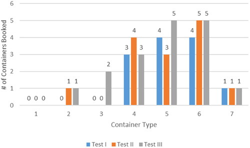
The proposed model determines the container booking plan for each region and at the hub at the first stage (see results in Table B1), and adjusts the bookings at the second stage if there are any unused containers to return or any urgent bookings on the day of shipping (see Table B2). We observe that containers of types 4, 5 and 6 are the preferred choices (see Figure 2) under all economic conditions. The explanation for this preference is the relative costs of the different types of container. Container types 4, 5, and 6 are less costly per unit volume than the larger types 1, 2, and 3 (see Table A1). However, although a container type 7 has a low cost per unit volume, it is not preferred. This is because space is wasted if this container type is used, due to the relative volumes of the container type and the cargo sizes.

Figure 2. Comparison of the total number of containers booked in poor, fair and good economic conditions.

4.2.2. Results on container loading plan

The experiments give optimal plans for booking of containers and loading of cargos in the regions and the hub under the different economic conditions. In the results, the small, medium and large cargos for Destination α are denoted by capital letters, S, M and L, and those for Destination β by small letters, s, m, and l. The results on how to load cargos into containers in each region are given in Table C1 of Appendix C; and results on the loading plans at the hub are summarised in Table C2 of Appendix C. Both are second-stage decisions in our proposed model.

Here we illustrate the Test III, good economy, results under different demand scenarios by Figure 3 (high demand), Figure 4 (medium demand), and Figure 5 (low demand). In each figure, containers loaded in Regions A and B are pre-booked containers. Information concerning the container type and the loading plans are shown under each container. Containers coloured in green in Region A will be “re-used” in the hub consolidation process and then transported further to the destinations. Similarly, containers coloured blue are also “re-used” containers, but they originate from Region B. Containers coloured yellow are pre-booked containers at the hub; containers coloured white at Region A and Region B will be used to transport cargos from regions to the hub but are not used in the hub consolidation process, and will then be kept by the airline company at no extra charge. Containers coloured in red are pre-booked containers at regions and hub, but will not be needed, i.e. “unused containers”, which will cause penalty charges by the airline company. We keep the container colours the same during the cargo forwarding process. In this manner, it is clear to see how the cargos are consolidated at the hub, and how each container is used in the cargo forwarding plans.

Figure 3. Cargo loading plan in good expected economic conditions under the high demand scenario. 1. Container colours represent pre-booked at A and re-used at hub (green), pre-booked at B and re-used at hub (blue), pre-booked at hub (yellow), pre-booked at A or B and not re-used (white), pre-booked and not used (red). 2. Cargo sizes, small (s, S), medium (m, M), large (l, L) are upper case to Destination α and lower case to β.

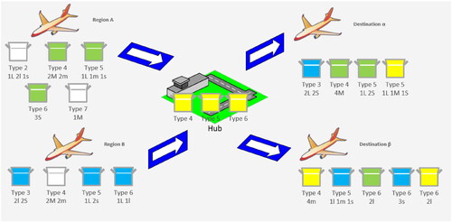
Figure 4. Cargo loading plan in good expected economic conditions under the medium demand scenario. 1. Container colours represent pre-booked at A and re-used at hub (green), pre-booked at B and re-used at hub (blue), pre-booked at hub (yellow), pre-booked at A or B and not re-used (white), pre-booked and not used (red). 2. Cargo sizes, small (s, S), medium (m, M), large (l, L) are upper case to Destination α and lower case to β.

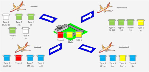
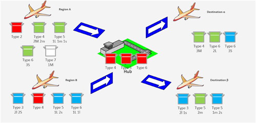
Figure 5. Cargo loading plan in good expected economic conditions under the low demand scenario. 1. Container colours represent pre-booked at A and re-used at hub (green), pre-booked at B and re-used at hub (blue), pre-booked at hub (yellow), pre-booked at A or B and not re-used (white), pre-booked and not used (red). 2. Cargo sizes, small (s, S), medium (m, M), large (l, L) are upper case to Destination α and lower case to β.

To illustrate how containerised cargos are transported from the hub to the destinations, we take results from Figure 3 as an example. In this high demand scenario, it can be observed that the type 4 container (green colour) from Region A will be used to carry 4 medium-sized cargos to Destination α; the type 3 container (blue colour) from Region B will be used to carry 2 large-sized cargos and 2 small-sized cargos to Destination α; one hub pre-booked container of type 4 will transport 4 medium-sized cargos to Destination β. There is no unused container in this scenario.

The results also include how cargos are loaded into each container in the regions, and identify if there are any pre-booked containers that are not utilised when demand is realised. Take the medium demand scenario as in Figure 4 as an example. At Region B, there will be one medium cargo with Destination β, one small cargo with Destination α and two small cargos with Destination β loaded into a type 3 container; one medium cargo with Destination α and one medium cargo with Destination β will be loaded into a type 5 container; one large cargo with Destination α and one large cargo with Destination β will be loaded into a type 6 container. There is one type 4 container (red colour) unused at Region B and also one in the hub unused container, both of which will be charged at the penalty costs. At Region A, a type 2 container and a type 7 container will carry cargos to the hub but not used to transport any further and kept by the airline company.

It may be noted from Figure 3 that in Test III, good expected economic conditions, with the high demand scenario there are pre-booked type 4 containers coming to the hub from both regions A and B. However, only one is re-used at the hub and an extra one is pre-booked at the hub. This may seem less than optimal: if both type 4 containers are re-used, there are discounts on both fixed rental costs. However, Figure 4 shows that in Test III, when good economic conditions are expected but the medium demand scenario is realised, one of the pre-booked type 4 containers is not used, thus incurring a penalty cost. This means that in Test III, the total number of re-usable type 4 containers, a first-stage decision, can be no more than 1. This highlights the possible disadvantage to the forwarder in having to make a decision about re-use of containers at the first stage, rather than at the second stage when demand is realised.

To investigate how cargos are packed at the regions and repacked in the hub for transporting to their final destinations, we use the low demand scenario as shown in Figure 5 as an example. With the low demand situation, there are more unused containers than expected, including one type 2 container pre-booked at Region A, one type 4 container pre-booked at Region B, and all the pre-booked containers at the hub; all these will be penalised by the airline company. The type 4 container at Region A carries 2 medium-sized cargos with Destination α and 2 medium-sized cargos with Destination β to the hub, where those cargos with Destination β are unloaded and one more medium-sized cargo (from type 7 container at Region A) will be loaded into this type 4 container. Therefore, this type 4 container (green colour) will take 3 medium-sized cargos to Destination α.

4.2.3. Results on all the related costs and computational efficiency

Next, we analyse all the related costs under the three economic conditions, comparing the fixed and variable rental costs, penalty costs for urgent booking/returning and the consolidation (repacking) costs. The costs are presented in Table 8. It can be concluded that under good economic conditions when the demand is most likely to be high, it is recommended by the model that more containers should be booked in the first stage to accommodate more cargos, so that there are no urgent booking costs. However, in fair and poor economic conditions, when demand is most likely to be at medium or low levels, then smaller numbers of containers should be booked in the first stage to avoid penalty costs of returning unused containers. Comparing the costs of good to those of fair and poor economic conditions, all the costs apart from penalty costs are higher, due to the high demand.

Table 8. Freight forwarder costs (in $) under three economic conditions (adapted from Zhu et al., 2015).

		Economic conditions
Stage	Costs	Test I: Poor	Test II: Fair	Test III: Good
First	Region pre-booked container rental	368,979	430,550	525,614
	Hub pre-booked container rental	74,820	106,353	145,238
	Hub re-used container rental	251,660	276,037	332,606
Second	Region cargo weight charge	24,694	36,703	56,921
	Hub cargo weight charge	4,673	12,950	21,087
	Hub re-used container cargo weight charge	21,592	30,163	40,877
	Region unused container return penalties	0	0	17,000
	Hub unused container return penalties	0	4000	17,500
	Region urgent container rental penalties	45,000	20,000	0
	Hub urgent container rental penalties	40,000	22,000	0
	Consolidation	34,800	40,300	49,600
	Total	866,217	979,056	1,206,444

Regarding the computational efficiency, the model returns results fastest, in 639 s, for the situation under poor economic conditions, while for the other conditions, it also works efficiently, taking 3877 and 36,621 s for fair and good conditions respectively. It can be noted that, for poor economic conditions, the problem size is smaller, so the computational time is shorter.

4.2.4. Further experiments on the impacts of scenario probabilities

In order to investigate the impacts of the demand scenario probabilities on the total costs, we carried out 10 sensitivity tests with different probabilities for high, medium and low demands (see results in Table 9). It can be concluded that the total costs depend highly on these probabilities, and higher costs are associated more with the probability for higher demands. This is because when the demand is high, there will be more containers needed, so the cost will go up.

Table 9. Comparing the total costs based on different scenario probabilities.

Demand			Total Costs
High	Medium	Low
10%	30%	60%	934543
10%	70%	20%	970601
15%	40%	45%	986906
20%	25%	55%	1011687
20%	60%	20%	1046089
30%	20%	50%	1075643
25%	65%	10%	1086928
35%	35%	30%	1113767
50%	25%	25%	1143335
75%	15%	10%	1197912

4.3. Computational results by GA

The model parameters settings are the same as the two-stage stochastic model. To find out the best combination values of GA parameters for our considered problem, we have designed a set of preliminary experiments in which the values of the following parameters change within the ranges below.

Maximum Generation [20,30,40,50]

Population Size [30,50,100,150,200,250]

Crossover rate [0.6,0.7,0.8,0.9]

Mutation rate [0.01,0.02,0.1,0.2]

Based on our observation, GA is able to find near-optimal solutions within 50 generations in all the cases. The size of population affects the quality of solution, and larger population leads to better solutions but takes more computation time; the effect of crossover and mutation rates on the solutions differs among cases. Therefore, we set the maximum generation 50, population size 200, crossover rate 0.7 and mutation rate 0.1 for the experiments below. The GA was run 30 times for each case and the average value is reported. The results from two-stage and three-stage models are presented in Tables 10 and 11. The costs obtained by the GA and the optimal costs obtained by the commercial software AIMMS are compared. It can be observed that in Test I, good economy environment, the gaps between the GA results and optimal solutions are the smallest. The computation times from AIMMS to get the optimal solutions range from 10 min to 10 h, while the solving time of the GA is less than 10 min in all our experiments.

Table 10. Comparison between GA and AIMMS for two-stage stochastic model.

Test	I	II	III
Total cost by GA	1288726	1067032	955656
Total cost by AIMMS	1206444	979056	866217
Gap between GA and AIMMS	6.82%	8.99%	10.33%
Computing time for AIMMS to get the optimal result (seconds)	36621.38	3876.64	639.34

Table 11. Comparison between GA and AIMMS for three-stage stochastic model.

Test	I	II	III
Total cost by AIMMS	2836720	2266843	2022581
Total cost by GA	2773415	2208467	1978423
Lower bound	2606252	2073880	1805892
Gap between AIMMS and Lower bound	8.12%	8.51%	10.71%
Gap between GA and Lower bound	6.03%	6.09%	8.72%
Computing time by AIMMS (seconds)	70860.69	46873.65	140961.85

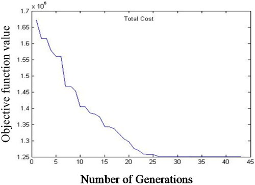
The convergency of the GA is shown in Figure 6, which demonstrates the evolvement of our proposed GA. The horizontal axis represents the number of generations in which the GA evolves, and the vertical axis represents the values of the objective function, i.e. the total costs.

Figure 6. Typical convergency process of the GA.

5. Conclusions

In this study, we have investigated the problem of forwarding cargos as international air freight via a hub, considering the processes of booking and loading air containers as well as consolidation of cargos in the hub. A stochastic programming model has been developed to deal with the uncertain demand by breaking the decisions into two stages, where the first stage decides the container bookings in each region and at the hub. At the second stage, on shipment day, the numbers of containers to be urgently booked or returned are decided, as well as container loading plans. We further extend the two-stage model into a multi-stage model. The main contribution of our research is that we combine all of these decisions and find solutions using a single model; the GA is designed to solve the problem in large sizes. This has not been addressed in previous studies. The proposed model has been tested by applying a real-world case study, and it has been shown that the model works efficiently in terms of providing detailed booking and loading plans, given different demand scenarios under various economic conditions. We have also demonstrated that the preferred air containers are those with smaller fixed costs per unit volume. Finally, an experiment on the demand probabilities has been carried out to show how the total costs are impacted by these probabilities. We conclude that the higher the demands are likely to be, the more total costs will be incurred.

The customer demands considered in our study can change only in terms of the quantities, i.e. the demand can be at low, medium and high levels. However, in reality, the demands can also change in terms of the requested shipping times, i.e. customers can request shipment of their cargos on dates different from their original plans: this is a possible future research direction. A second area for future research is to use efficient approaches to generate and model scenarios; for example Monte Carlo simulation, machine learning and other predictive analytics methods can be used for creating scenarios, and probability theory and fuzzy theory can be applied to model scenarios. Another area is to take into consideration the multi-hub case, where international cargos can be consolidated at different hubs before reaching their final destinations, while combining the transportation scheduling, i.e. deliveries of cargos by trucks and airline schedules, into the cargo forwarding plans.

Disclosure Statement

No potential conflict of interest was reported by the author(s).

Appendix A:

Model inputs

Appendix B:

Results on container booking plans for all the scenarios (adapted from Zhu et al., 2015)

Table B1. Container advance booking plans at each region and at the hub under each economic condition (first-stage decisions).

Container type				1	2	3	4	5	6	7
Economic Conditions	Test I:	Region Pre-booked	A				1	1	1
	Poor		B				1	1	1
		Hub Re-used					1	2	2
		Hub Pre-booked								1
	Test II: Fair	Region Pre-booked	A		1		1		1	1
			B				1	1	1
		Hub Re-used					2	1	2
		Hub Pre-booked						1	1
	Test III:	Region Pre-booked	A		1		1	1	1	1
	Good		B			1	1	1	1
		Hub Re-used				1	1	2	2
		Hub Pre-booked					1	1	1

When first stage decisions are made, the future demand is unknown: this can only be known on shipment day, thus affecting decisions taken at the second stage. The three tests represent poor, fair and good economic conditions, respectively, given the expected view of demand. Taking Test III, good economic conditions, as an example from Table B1: Region A will pre-book air containers of types 2, 4, 5, 6, and 7; in Region B there will be pre-booking of air containers of types 3, 4, 5, and 6; at the hub, a type 3, a type 4, two type 5 containers and two type 6 containers will be re-used; in addition, extra type 4, 5 and 6 containers are pre-booked at the hub. All the other cases can be described in a similar way.

Table B2. Urgent booking of containers and returning of unused containers in regions and at hub on shipment day (second-stage decisions), (adapted from Zhu et al., 2015).

					Demand scenario realised at stage 2
					Low demand, s1					Medium demand, s2		High demand, s3
					2	3	4	5	6	3	4	2	3	4	5	7
Economic conditions expected at stage 1	Test I: Poor	Urgent	Region	A						x		x				x
				B									x
			Hub								x		x	x	x
		Unused	Region	A
				B
			Hub
	Test II: Fair	Urgent	Region	A											x
				B									x
			Hub			x	x
		Unused	Region	A
				B
			Hub					x
	Test III: Good	Urgent	Region	A
				B
			Hub
		Unused	Region	A	x
				B			x				x
			Hub				x	x	x		x

Once the actual demands are realised, the model returns the results on the second-stage decisions. When the economic condition is expected to be good, most of the cases with returning the unused containers will occur in the scenario of low realised demands, as shown in Table B2, in which x indicates one container involved. In contrast, when the economic condition is expected to be poor, yet the demand level is high, i.e. scenario 3 is realised, extra containers are needed for urgent bookings in the regions and at the hub. Combining the results from Tables B1 and B2, it can be observed that when good economic conditions are expected, when it is most likely (with 80% probability) that high demand occurs, there will be more containers booked at the first stage (see Test III for good economic conditions in Table B1) and no urgent booking in the second stage (see Test III, good economic conditions, urgent section in Table B2).

Appendix C:

Cargo loading plan results under test I, good economic conditions (Zhu et al., 2015)

Table C1. Regional assignment of cargos to container type by demand scenario.

			Cargo loading by container type
			1	2	3	4	5	6	7
Scenario	Low demand	Region A	0	0	0	2M 1 m	1m 2S	1L 1 l	1s
		Region B	0	0	1l 1 M 1 s	0	1m 1 s	1L 1S	0
	Medium demand	Region A	0	1l 2 M 1 s	0	3m	2S	2L	1s
		Region B	0	0	1m 1S 2 s	0	2M 1 m	1L 1 l	0
	High demand	Region A	0	1L 2 l 1 s	0	2M 2 m	1L 1 m 1 s	3S	1M
		Region B	0	0	2l 2S	2M 2 m	1L 2 s	1L 1 l	0

Table C2. Plans for loading cargo in the hub for different destinations using different container types.

			Demand scenario
			Low		Medium		High
			Destn α	Destn β	Destn α	Destn β	Destn α	Destn β
Container type	3	From Region B		2l 1 s		2l 1 m	2L 2S
	4	From Region A	3M		1L 2 M		4M
		From hub						4m
	5	From Region A		2m	2M		1L 2S
		From Region B		1m 2 s		2m		1l 1 m 1 s
		From hub				2m 1 s	1L 1 M 1S
	6	From Region A	2L		3S			2l
		From Region B	3S			3s		3s
		From hub			2L			2l

Appendix D:

The multi-stage stochastic model

To extend our proposed two-stage model into a multi-stage model, index t is added to represent the periods, where t= {1,2,…,T}. All the other notations are the multi-stage versions of the two-stage variables. Compared to the two-stage model, this multi-stage model allows the relevant decisions to be adjusted at multiple times during the whole planning horizon, thus achieving the greatest cost efficiency overall. (D.1) $$\mathrm{min }\sum _{t=1}^T(\sum _{s_1}^S\sum _{s_2}^S\cdots \sum _{s_t}^S{p}_{\left(s_1{s}_2\cdots s_t\right)}(\sum _{r=1}^R{M}_{rt}+N_t)\mathrm{ }$$(D.1) subject to (D.2) $$M_{rt}=\sum _{i=1}^m\sum _{l=1}^{L_{\mathit{irt}}}{c}_{\mathit{irt}}^0{x}_{\mathit{ilr}\left(s_1{s}_2\cdots s_t\right)}+\sum _{i=1}^m\sum _{l=1}^{L_{\mathit{irt}}}\sum _{k=1}^{K_i}{\delta }_{\mathit{ikr}}{g}_{\mathit{ilkr}\left(s_1{s}_2\cdots s_t\right)}+\sum _{i=1}^m{c}_{\mathit{irt}}^{-}{o}_{ir\left(s_1{s}_2\cdots s_t\right)}^{-}+\sum _{i=1}^m{c}_{\mathit{irt}}^{+}{o}_{ir\left(s_1{s}_2\cdots s_t\right)}^{+}+\sum _{d=1}^D\sum _{j=1}^n{b}_{\mathit{jrt}}^{+}{y}_{\mathit{jrd}\left(s_1{s}_2\cdots s_t\right)}^{+}+\sum _{r=1}^R\sum _{i=1}^m\sum _{l=1}^{L_{\mathit{irt}}}{b}_{it}{x}_{\mathit{ilr}\left(s_1{s}_2\cdots s_t\right)}\mathrm{ }$$(D.2) (D.3) $$N_t=\sum _{d=1}^D(\sum _{i=1}^m\sum _{l=1}^{L_{it}}\mu c_{it}^{h0}{x}_{\mathit{ild}{(s}_1{s}_2\cdots s_t)}^{hc}+\sum _{i=1}^m\sum _{l=1}^{L_{it}}\sum _{k=1}^{K_i}{\delta }_{ik}^h{g}_{i\mathrm{l}kd{(s}_1{s}_2\cdots s_t)}^{hc}+\sum _{i=1}^m\sum _{l=1}^{L_{it}^h}{c}_{it}^{h0}{x}_{\mathit{ild}(s_1{s}_2\cdots s_t)}^h+\sum _{i=1}^m\sum _{l=1}^{L_{it}^h}\sum _{k=1}^{K_i}{\delta }_{ik}^h{g}_{\mathit{ilkd}(s_1{s}_2\cdots s_t)}^h+\sum _{j=1}^n{b}_{jt}^{h+}{y}_{jd(s_1{s}_2\cdots s_t)}^{h+})+\sum _{i=1}^m{c}_{it}^{h-}{o}_{i(s_1{s}_2\cdots s_t)}^{h-}+\sum _{i=1}^m{c}_{it}^{h+}{o}_{i(s_1{s}_2\cdots s_t)}^{h+}\mathrm{ }$$(D.3) (D.4) $$\sum _{j=1}^n\sum _{d=1}^D{v}_j{y}_{\mathit{iljrd}{(s}_1{s}_2\cdots s_t)}\mathrm{ }\le V_i{x}_{\mathit{ilr}{(s}_1{s}_2\cdots s_t)}\mathrm{ }i=1,\mathrm{ }\cdots ,m;\mathrm{ }l=1,\mathrm{ }\cdots ,\mathrm{ }{L}_{\mathit{irt}};\mathrm{ }t=1,\dots ,T;s_1,\mathrm{ }\cdots ,s_t=1,\mathrm{ }\cdots ,\mathrm{ }S;\mathrm{ }r=1,\mathrm{ }\cdots ,\mathrm{ }R;\mathrm{ }$$(D.4) (D.5) $$\sum _{j=1}^n\sum _{d=1}^D{w}_j{y}_{\mathit{iljrd}{(s}_1{s}_2\cdots s_t)}\le W_i{x}_{\mathit{ilr}{(s}_1{s}_2\cdots s_t)}\mathrm{ }i=1,\mathrm{ }\cdots ,m;\mathrm{ }l=1,\mathrm{ }\cdots ,\mathrm{ }{L}_{\mathit{irt}};\mathrm{ }t=1,\dots ,T;\mathrm{ }{s}_1,\mathrm{ }\cdots ,s_t=1,\mathrm{ }\cdots ,\mathrm{ }S;\mathrm{ }r=1,\mathrm{ }\cdots ,\mathrm{ }R;\mathrm{ }$$(D.5) (D.6) $$\sum _{j=1}^n{v}_j{y}_{\mathit{iljd}{(s}_1{s}_2\cdots s_t)}^h\le V_i{x}_{\mathit{ild}{(s}_1{s}_2\cdots s_t)}^h\mathrm{ }i=1,\mathrm{ }\cdots ,m;\mathrm{ }l=1,\mathrm{ }\cdots ,\mathrm{ }{L}_{it}^h;\mathrm{ }t=1,\dots ,T;\mathrm{ }{s}_1,\mathrm{ }\cdots ,s_t=1,\mathrm{ }\cdots ,\mathrm{ }S;\mathrm{ }d=1,\mathrm{ }\cdots ,\mathrm{ }D;$$(D.6) (D.7) $$\sum _{j=1}^n{w_{j}y}_{\mathit{iljd}{(s}_1{s}_2\cdots s_t)}^h\le W_i{x}_{\mathit{ild}{(s}_1{s}_2\cdots s_t)}^h\mathrm{ }i=1,\mathrm{ }\cdots ,m;\mathrm{ }l=1,\mathrm{ }\cdots ,\mathrm{ }{L}_{it}^h;\mathrm{ }t=1,\dots ,T;\mathrm{ }{s}_1,\mathrm{ }\cdots ,s_t=1,\mathrm{ }\cdots ,\mathrm{ }S;\mathrm{ }d=1,\mathrm{ }\cdots ,\mathrm{ }D;\mathrm{ }$$(D.7) (D.8) $$\sum _{j=1}^n{v}_j{y}_{\mathit{iljd}{(s}_1{s}_2\cdots s_t)}^{hc}\le V_i{x}_{\mathit{ild}{(s}_1{s}_2\cdots s_t)}^{hc}\mathrm{ }i=1,\mathrm{ }\cdots ,m;\mathrm{ }l=1,\mathrm{ }\cdots ,\mathrm{ }{L}_{it};\mathrm{ }t=1,\dots ,T;\mathrm{ }{s}_1,\mathrm{ }\cdots ,s_t=1,\mathrm{ }\cdots ,\mathrm{ }S;\mathrm{ }d=1,\mathrm{ }\cdots ,\mathrm{ }D;\mathrm{ }$$(D.8) (D.9) $$\sum _{j=1}^n{w_{j}y}_{\mathit{iljd}{(s}_1{s}_2\cdots s_t)}^{hc}\le W_i{x}_{\mathit{ild}{(s}_1{s}_2\cdots s_t)}^{hc}\mathrm{ }i=1,\mathrm{ }\cdots ,m;\mathrm{ }l=1,\mathrm{ }\cdots ,\mathrm{ }{L}_{it};\mathrm{ }t=1,\dots ,T;\mathrm{ }{s}_1,\mathrm{ }\cdots ,s_t=1,\mathrm{ }\cdots ,\mathrm{ }S;\mathrm{ }d=1,\mathrm{ }\cdots ,\mathrm{ }D;\mathrm{ }$$(D.9) (D.10) $$y_{\mathit{jrd}{s}_0}^{+}=0,\mathrm{ }{y}_{\mathit{jrd}\left(s_1{s}_2\cdots s_T\right)}^{+}=0\mathrm{ }j=1,\mathrm{ }\cdots ,\mathrm{ }n;\mathrm{ }r=1,\mathrm{ }\cdots ,\mathrm{ }R;\mathrm{ }d=1,\mathrm{ }\cdots ,\mathrm{ }D\mathrm{ }$$(D.10) (D.11) $$\sum _{i=1}^m\sum _{d=1}^D\sum _{l=1}^{L_{\mathit{irt}}}{y}_{i\mathrm{l}\mathit{jrd}\left(s_1{s}_2\cdots s_t\right)}+\sum _{d=1}^D{y}_{\mathit{jrd}\left(s_1{s}_2\cdots s_t\right)}^{+}=q_{jr\left(s_1{s}_2\cdots s_t\right)}+\sum _{d=1}^D{y}_{\mathit{jrd}\left(s_1{s}_2\cdots s_{t-1}\right)}^{+}\mathrm{ }j=1,\mathrm{ }\cdots ,\mathrm{ }n;\mathrm{ }r=1,\mathrm{ }\cdots ,\mathrm{ }R;\mathrm{ }t=1,\dots ,T;\mathrm{ }{s}_1,\dots ,s_t=1,\dots ,S\mathrm{ }$$(D.11) (D.12) $$y_{\mathit{jrd}\left(s_1{s}_2\cdots s_t\right)}^{+}\le \sum _{i=1}^m\sum _{l=1}^{L_{\mathit{irt}}}{y}_{\mathit{iljrd}\left(s_1{s}_2\cdots s_{t+1}\right)}\mathrm{ }j=1,\mathrm{ }\cdots ,\mathrm{ }n;r=1,\mathrm{ }\cdots ,\mathrm{ }R;\mathrm{ }d=1,\mathrm{ }\cdots ,\mathrm{ }D;\mathrm{ }t=1,\dots ,T;\mathrm{ }{s}_1,\dots ,s_t=1,\dots ,S\mathrm{ }$$(D.12) (D.13) $$y_{jd{s}_0}^{h+}=0,\mathrm{ }{y}_{jd\left(s_1{s}_2\cdots s_T\right)}^{h+}=0\mathrm{ }j=1,\mathrm{ }\cdots ,\mathrm{ }n;\mathrm{ }d=1,\mathrm{ }\cdots ,\mathrm{ }D\mathrm{ }$$(D.13) (D.14) $$\sum _{i=1}^m\sum _{l=1}^{L_{it}^h}{y}_{\mathit{iljd}\left(s_1{s}_2\cdots s_t\right)}^h+\sum _{i=1}^m\sum _{l=1}^{L_{it}}{y}_{\mathit{iljd}\left(s_1{s}_2\cdots s_t\right)}^{hc}+y_{jd\left(s_1{s}_2\cdots s_t\right)}^{h+}=q_{jd\left(s_1{s}_2\cdots s_t\right)}^h+y_{jd\left(s_1{s}_2\cdots s_{t-1}\right)}^{h+}-\sum _{r=1}^R{y}_{\mathit{jrd}\left(s_1{s}_2\cdots s_t\right)}^{+}\mathrm{ }j=1,\mathrm{ }\cdots ,\mathrm{ }n;\mathrm{ }d=1,\mathrm{ }\cdots ,\mathrm{ }D;\mathrm{ }t=1,\dots ,T;s_1,\dots ,s_t=1,\dots ,S\mathrm{ }$$(D.14) (D.15) $$y_{jd\left(s_1{s}_2\cdots s_t\right)}^{h+}\le \sum _{i=1}^m\sum _{l=1}^{L_{it}^h}{y}_{\mathit{ilj}\left(s_1{s}_2\cdots s_{t+1}\right)}^h+\sum _{i=1}^m\sum _{l=1}^{L_{it}}{y}_{\mathit{iljd}\left(s_1{s}_2\cdots s_{t+1}\right)}^{hc}\mathrm{ }j=1,\mathrm{ }\cdots ,\mathrm{ }n;\mathrm{ }d=1,\mathrm{ }\cdots ,\mathrm{ }D;\mathrm{ }t=1,\dots ,T-1;{\mathrm{ }s}_1,\dots ,s_t=1,\dots ,S\mathrm{ }$$(D.15) (D.16) $$o_{\mathit{irt}}=\sum _{l=1}^{L_{\mathit{irt}}}{x}_{\mathit{ilr}{(s}_1{s}_2\cdots s_t)}+o_{ir{(s}_1{s}_2\cdots s_t)}^{+}-o_{ir{(s}_1{s}_2\cdots s_t)}^{-}\mathrm{ }i=1,\mathrm{ }\cdots ,m;\mathrm{ }r=1,\mathrm{ }\cdots ,\mathrm{ }R,\mathrm{ }t=1,\dots ,T;{\mathrm{ }s}_1,\dots ,s_t=1,\dots ,S\mathrm{ }$$(D.16) (D.17) $$o_{it}^h=\sum _{l=1}^{L_{it}^h}\sum _{d=1}^D{x}_{\mathit{ild}{(s}_1{s}_2\cdots s_t)}^h+o_{i{(s}_1{s}_2\cdots s_t)}^{h+}-o_{i{(s}_1{s}_2\cdots s_t)}^{h-}\mathrm{ }i=1,\mathrm{ }\cdots ,m;\mathrm{ }t=1,\dots ,T;\mathrm{ }{s}_1,\dots ,s_t=1,\dots ,S\mathrm{ }$$(D.17) (D.18) $$\sum _{r=1}^R\sum _{l=1}^{L_{\mathit{irt}}}{x}_{\mathit{ild}{(s}_1{s}_2\cdots s_t)}^{hc}\le \sum _{r=1}^R\sum _{l=1}^{L_{\mathit{irt}}}{x}_{\mathit{ilr}{(s}_1{s}_2\cdots s_t)}\mathrm{ }i=1,\mathrm{ }\cdots ,m;\mathrm{ }t=1,\dots ,T;\mathrm{ }{s}_1,\dots ,s_t=1,\dots ,S\mathrm{ }$$(D.18) (D.19) $$\sum _{l=1}^{L_{it}^h}\sum _{d=1}^D{x}_{\mathit{ild}{(s}_1{s}_2\cdots s_t)}^h\le L_{it}^h\mathrm{ }i=1,\mathrm{ }\cdots ,m;\mathrm{ }t=1,\dots ,T;\mathrm{ }{s}_1,\dots ,s_t=1,\dots ,S\mathrm{ }$$(D.19) (D.20) $$\sum _{r=1}^R\sum _{l=1}^{L_{\mathit{irt}}}\sum _{d=1}^D{x}_{\mathit{ild}{(s}_1{s}_2\cdots s_t)}^{hc}=o_{it}^{hc}\mathrm{ }i=1,\mathrm{ }\cdots ,m;\mathrm{ }t=1,\dots ,T;\mathrm{ }{s}_1,\dots ,s_t=1,\dots ,S$$(D.20) (D.21) $$\sum _{k=1}^{K_i}{g}_{\mathit{ilkr}{(s}_1{s}_2\cdots s_t)}=\sum _{j=1}^n\sum _{d=1}^D{w}_j{y}_{\mathit{iljrd}{(s}_1{s}_2\cdots s_t)}\mathrm{ }i=1,\mathrm{ }\cdots ,m;\mathrm{ }l=1,\mathrm{ }\cdots ,\mathrm{ }{L}_{\mathit{irt}};\mathrm{ }t=1,\dots ,T;\mathrm{ }{s}_1,\dots ,s_t=1,\dots ,S;\mathrm{ }r=1,\mathrm{ }\cdots ,\mathrm{ }R\mathrm{ }$$(D.21) (D.22) $$g_{\mathit{ilkr}{(s}_1{s}_2\cdots s_t)}\le z_{\mathit{ilkr}{(s}_1{s}_2\cdots s_t)}\left(a_{\mathit{ikr}}-a_{i\left(k-1\right)r}\right)\mathrm{ }i=1,\mathrm{ }\cdots ,m;\mathrm{ }l=1,\mathrm{ }\cdots ,\mathrm{ }{L}_{\mathit{irt}};\mathrm{ }k=1,\mathrm{ }\cdots ,\mathrm{ }{K}_i;\mathrm{ }t=1,\dots ,T;\mathrm{ }r=1,\mathrm{ }\cdots ,\mathrm{ }R;\mathrm{ }{s}_1,\dots ,s_t=1,\dots ,S\mathrm{ }$$(D.22) (D.23) $$g_{\mathit{ilkr}{(s}_1{s}_2\cdots s_t)}\ge z_{il(k-1)r{(s}_1{s}_2\cdots s_t)}\left(a_{\mathit{ikr}}-a_{i\left(k-1\right)r}\right)\mathrm{ }i=1,\mathrm{ }\cdots ,m;\mathrm{ }l=1,\mathrm{ }\cdots ,\mathrm{ }{L}_{\mathit{irt}};\mathrm{ }k=1,\mathrm{ }\cdots ,\mathrm{ }{K}_i;\mathrm{ }t=1,\dots ,T;\mathrm{ }r=1,\mathrm{ }\cdots ,\mathrm{ }R;\mathrm{ }{s}_1,\dots ,s_t=1,\dots ,S\mathrm{ }$$(D.23) (D.24) $$\sum _{k=1}^{K_i}{g}_{\mathit{ilkd}{(s}_1{s}_2\cdots s_t)}^h=\sum _{j=1}^n{y}_{\mathit{iljd}{(s}_1{s}_2\cdots s_t)}^h\mathrm{ }i=1,\mathrm{ }\cdots ,m;\mathrm{ }l=1,\mathrm{ }\cdots ,\mathrm{ }{L}_{it}^h;\mathrm{ }t=1,\dots ,T;\mathrm{ }d=1,\mathrm{ }\cdots ,\mathrm{ }D;\mathrm{ }{s}_1,\dots ,s_t=1,\dots ,S$$(D.24) (D.25) $$g_{\mathit{ilkd}{(s}_1{s}_2\cdots s_t)}^h\le z_{\mathit{ilkd}{(s}_1{s}_2\cdots s_t)}^h\left(a_{ik}^h-a_{i\left(k-1\right)}^h\right)\mathrm{ }i=1,\mathrm{ }\cdots ,m;\mathrm{ }l=1,\mathrm{ }\cdots ,\mathrm{ }{L}_{it}^h;\mathrm{ }t=1,\dots ,T;\mathrm{ }k=1,\mathrm{ }\cdots ,\mathrm{ }{K}_i;\mathrm{ }{s}_1,\dots ,s_t=1,\dots ,S\mathrm{ }$$(D.25) (D.26) $$g_{\mathit{ilkd}{(s}_1{s}_2\cdots s_t)}^h\ge z_{il(k-1)d{(s}_1{s}_2\cdots s_t)}^h\left(a_{ik}^h-a_{i\left(k-1\right)}^h\right)\mathrm{ }i=1,\mathrm{ }\cdots ,m;\mathrm{ }l=1,\mathrm{ }\cdots ,\mathrm{ }{L}_{it}^h;\mathrm{ }t=1,\dots ,T;\mathrm{ }k=1,\mathrm{ }\cdots ,\mathrm{ }{K}_i;\mathrm{ }{s}_1,\dots ,s_t=1,\dots ,S\mathrm{ }$$(D.26) (D.27) $$\sum _{k=1}^{K_i}{g}_{\mathit{ilkd}{(s}_1{s}_2\cdots s_t)}^{hc}=\sum _{j=1}^n{y}_{\mathit{iljd}{(s}_1{s}_2\cdots s_t)}^{hc}\mathrm{ }i=1,\mathrm{ }\cdots ,m;\mathrm{ }l=1,\mathrm{ }\cdots ,\mathrm{ }{L}_{it}^h;\mathrm{ }t=1,\dots ,T;\mathrm{ }d=1,\mathrm{ }\cdots ,\mathrm{ }D;\mathrm{ }{s}_1,\dots ,s_t=1,\dots ,S\mathrm{ }$$(D.27) (D.28) $$g_{\mathit{ilkd}{(s}_1{s}_2\cdots s_t)}^{hc}\le z_{\mathit{ilkd}{(s}_1{s}_2\cdots s_t)}^{hc}\left(a_{ik}^h-a_{i\left(k-1\right)}^h\right)\mathrm{ }i=1,\mathrm{ }\cdots ,m;\mathrm{ }l=1,\mathrm{ }\cdots ,\mathrm{ }{L}_{\mathit{irt}};\mathrm{ }t=1,\dots ,T;\mathrm{ }k=1,\mathrm{ }\cdots ,\mathrm{ }{K}_i;\mathrm{ }r=1,\mathrm{ }\cdots ,\mathrm{ }R;\mathrm{ }{s}_1,\dots ,s_t=1,\dots ,S\mathrm{ }$$(D.28) (D.29) $$g_{\mathit{ilkd}{(s}_1{s}_2\cdots s_t)}^{hc}\ge z_{il(k-1)d{(s}_1{s}_2\cdots s_t)}^{hc}\left(a_{ik}^h-a_{i\left(k-1\right)}^h\right)\mathrm{ }i=1,\mathrm{ }\cdots ,m;\mathrm{ }l=1,\mathrm{ }\cdots ,\mathrm{ }{L}_{\mathit{irt}};\mathrm{ }t=1,\dots ,T;\mathrm{ }k=1,\mathrm{ }\cdots ,\mathrm{ }{K}_i;\mathrm{ }r=1,\mathrm{ }\cdots ,\mathrm{ }R;\mathrm{ }{s}_1,\dots ,s_t=1,\dots ,S\mathrm{ }$$(D.29) (D.30) $$\begin{array}{l}\begin{array}{c}{o}_{\mathit{irt}},\mathrm{ }{o}_{ir{(s}_1{s}_2\cdots s_t)}^{-},\mathrm{ }{o}_{ir{(s}_1{s}_2\cdots s_t)}^{+},o_{it}^h,\mathrm{ }{o}_{i{(s}_1{s}_2\cdots s_t)}^{h-},\mathrm{ }{o}_{i{(s}_1{s}_2\cdots s_t)}^{h+},\mathrm{ }{o}_{it}^{hc},\mathrm{ }{y}_{\mathit{iljrd}{(s}_1{s}_2\cdots s_t)},\mathrm{ }{y}_{\mathit{jrd}\left(s_1{s}_2\cdots s_t\right)}^{+},\mathrm{ }{y}_{\mathit{iljd}{(s}_1{s}_2\cdots s_t)}^h,\\ y_{\mathit{ilj}{d(s}_1{s}_2\cdots s_t)}^{hc},\mathrm{ }{y}_{jd\left(s_1{s}_2\cdots s_t\right)}^{h+},\mathrm{ }{g}_{\mathit{ilkr}{(s}_1{s}_2\cdots s_t)},\mathrm{ }{g}_{\mathit{ilkd}{(s}_1{s}_2\cdots s_t)}^h,\mathrm{ }{g}_{\mathit{ilkd}{(s}_1{s}_2\cdots s_t)}^{hc}\in \left\{0,1,\dots ,\inf \right\};\mathrm{ }{x}_{\mathit{ilr}{(s}_1{s}_2\cdots s_t)},\\ x_{\mathit{ild}{(s}_1{s}_2\cdots s_t)}^h,\mathrm{ }{x}_{\mathit{ild}{(s}_1{s}_2\cdots s_t)}^{hc},\mathrm{ }{z}_{\mathit{ilkr}{(s}_1{s}_2\cdots s_t)},\mathrm{ }{z}_{\mathit{ilkd}{(s}_1{s}_2\cdots s_t)}^h,\mathrm{ }{z}_{\mathit{ilkd}{(s}_1{s}_2\cdots s_t)}^{hc}\mathrm{ }\in \left\{0,1\right\}\mathrm{ }i=1,\mathrm{ }\cdots ,m,\end{array}{o}_{\mathit{irt}},\mathrm{ }{o}_{ir{(s}_1{s}_2\cdots s_t)}^{-},\mathrm{ }{o}_{ir{(s}_1{s}_2\cdots s_t)}^{+},o_{it}^h,\mathrm{ }{o}_{i{(s}_1{s}_2\cdots s_t)}^{h-},\mathrm{ }{o}_{i{(s}_1{s}_2\cdots s_t)}^{h+},\mathrm{ }{o}_{it}^{hc},\mathrm{ }{y}_{\mathit{iljrd}{(s}_1{s}_2\cdots s_t)},\mathrm{ }{y}_{\mathit{jrd}\left(s_1{s}_2\cdots s_t\right)}^{+},\mathrm{ }{y}_{\mathit{iljd}{(s}_1{s}_2\cdots s_t)}^h,\\ l=1,\mathrm{ }\cdots ,\mathrm{ }{L}_{\mathit{irt}};\mathrm{ }j=1,\mathrm{ }\cdots ,n;\mathrm{ }r=1,\mathrm{ }\cdots ,\mathrm{ }R;\mathrm{ }d=1,\mathrm{ }\cdots ,\mathrm{ }D,\mathrm{ }t=1,\dots ,T;\mathrm{ }k=1,\mathrm{ }\cdots ,\mathrm{ }{K}_i;\mathrm{ }{s}_1,\dots ,s_t=1,\dots ,S\mathrm{ }\end{array}$$(D.30)

The objective function (D.1) is the total cost including container fixed and variable costs in the regions, penalty costs for renting or returning containers on the shipping day in the regions, inventory costs in regions, repacking costs in the hub, fixed and variable costs for the pre-used containers and new containers in the hub, inventory costs in the hub and uncertainty costs for renting or returning containers to the hub. The details of the objective function can be found in the constraints (D.2) and (D.3). Constraints (D.4)(D.4) $$\sum _{j=1}^n\sum _{d=1}^D{v}_j{y}_{\mathit{iljrd}{(s}_1{s}_2\cdots s_t)}\mathrm{ }\le V_i{x}_{\mathit{ilr}{(s}_1{s}_2\cdots s_t)}\mathrm{ }i=1,\mathrm{ }\cdots ,m;\mathrm{ }l=1,\mathrm{ }\cdots ,\mathrm{ }{L}_{\mathit{irt}};\mathrm{ }t=1,\dots ,T;s_1,\mathrm{ }\cdots ,s_t=1,\mathrm{ }\cdots ,\mathrm{ }S;\mathrm{ }r=1,\mathrm{ }\cdots ,\mathrm{ }R;\mathrm{ }$$(D.4) –(D.9) ensure that the cargoes loaded into the containers cannot exceed the volume and weight limitations. The cargo quantity constraints in the regions and hub are (D.10)–(D.15). (D.10) and (D.13) mean that quantities of stored cargo before the first period and in the final period must be 0. (D. 11) and (D.14) ensure that the all the cargoes are transported throughout the process. (D.12) and (D.15) mean the quantity of storage cargo in any period is less than or equal to the quantity of transported cargo in the next. These two constraints enable the assumption that the air cargoes can be transported with one day’s delay. If the assumption should be changed to two days or more, we just need to change these two constraints. The container quantity constraints in the regions and hub are (D.16) and (D.17). Constraint (D.18) means that for each type of container, the quantity of pre-used containers used in the hub cannot be greater than the sum of containers used in all regions. Constraint (D.19) ensures that the number of each type of container used in the hub cannot exceed the limit. Constraint (D.20) makes sure that the pre-used container usage plan is the same no matter which scenario is realised. Constraints (D.21)–(D.29) are container variable cost constraints. Constraint (D.30) is the variable range.

References

- Bookbinder, J. H., Elhedhli, S., & Li, Z. (2015). The air-cargo consolidation problem with pivot weight: Models and solution methods. Computers & Operations Research, 59, 22–32. https://doi.org/10.1016/j.cor.2014.11.015
- Bookbinder, J. H., & Higginson, J. K. (2002). Probabilistic modeling of freight consolidation by private carriage. Transportation Research Part E: Logistics and Transportation Review, 38(5), 305–318. https://doi.org/10.1016/S1366-5545(02)00014-5
- Bortfeldt, A., & Wäscher, G. (2013). Constraints in container loading–A state-of-the-art review. European Journal of Operational Research, 229(1), 1–20. https://doi.org/10.1016/j.ejor.2012.12.006
- Brandt, F., & Nickel, S. (2019). The air cargo load planning problem-a consolidated problem definition and literature review on related problems. European Journal of Operational Research, 275(2), 399–410. https://doi.org/10.1016/j.ejor.2018.07.013
- Chan, F. T., Bhagwat, R., Kumar, N., Tiwari, M., & Lam, P. (2006). Development of a decision support system for air-cargo pallets loading problem: A case study. Expert Systems with Applications, 31(3), 472–485. https://doi.org/10.1016/j.eswa.2005.09.057
- Chao, C.-C., & Li, R.-G. (2017). Effects of cargo types and load efficiency on airline cargo revenues. Journal of Air Transport Management, 61, 26–33. https://doi.org/10.1016/j.jairtraman.2015.11.006
- Chew, E.-P., Huang, H.-C., Johnson, E. L., Nemhauser, G. L., Sokol, J. S., & Leong, C.-H. (2006). Short-term booking of air cargo space. European Journal of Operational Research, 174(3), 1979–1990. https://doi.org/10.1016/j.ejor.2005.05.011
- Delgado, F., Trincado, R., & Pagnoncelli, B. K. (2019). A multistage stochastic programming model for the network air cargo allocation under capacity uncertainty. Transportation Research Part E: Logistics and Transportation Review, 131, 292–307. https://doi.org/10.1016/j.tre.2019.09.011
- Feng, B., Li, Y., & Shen, Z.-J. M. (2015). Air cargo operations: Literature review and comparison with practices. Transportation Research Part C: Emerging Technologies, 56, 263–280. https://doi.org/10.1016/j.trc.2015.03.028
- Guéret, C., Jussien, N., Lhomme, O., Pavageau, C., & Prins, C. (2003). Loading aircraft for military operations. Journal of the Operational Research Society, 54(5), 458–465. https://doi.org/10.1057/palgrave.jors.2601551
- Ha, H. T. H., & Nananukul, N. (2017). Air cargo optimization models for logistics forwarders. Advanced Science Letters, 23(5), 4162–4167. https://doi.org/10.1166/asl.2017.8327
- Huang, K., & Chi, W. (2007). A Lagrangian relaxation based heuristic for the consolidation problem of airfreight forwarders. Transportation Research Part C: Emerging Technologies, 15(4), 235–245. https://doi.org/10.1016/j.trc.2006.08.006
- Huang, K., Lee, Y.-T., & Xu, H. (2020). A routing and consolidation decision model for containerized air-land intermodal operations. Computers & Industrial Engineering, 141, 106299. https://doi.org/10.1016/j.cie.2020.106299
- Leung, L. C., Hui, Y. V., Chen, G., & Wong, W. H. (2017). Aggregate-disaggregate approach to an airfreight forwarder's planning under uncertainty: A case study. Journal of the Operational Research Society, 68(6), 695–710. https://doi.org/10.1057/s41274-016-0124-0
- Leung, L. C., Van Hui, Y., Wang, Y., & Chen, G. (2009). A 0–1 LP model for the integration and consolidation of air cargo shipments. Operations Research, 57(2), 402–412. https://doi.org/10.1287/opre.1080.0583
- Li, Y., Tao, Y., & Wang, F. (2009). A compromised large-scale neighborhood search heuristic for capacitated air cargo loading planning. European Journal of Operational Research, 199(2), 553–560. https://doi.org/10.1016/j.ejor.2008.11.033
- Limbourg, S., Schyns, M., & Laporte, G. (2012). Automatic aircraft cargo load planning. Journal of the Operational Research Society, 63(9), 1271–1283. https://doi.org/10.1057/jors.2011.134
- Lin, C.-C., & Chen, Y.-C. (2003). The integration of Taiwanese and Chinese air networks for direct air cargo services. Transportation Research Part A: Policy and Practice, 37(7), 629–647.
- Nance, R., Roesener, A., & Moore, J. (2011). An advanced tabu search for solving the mixed payload airlift loading problem. Journal of the Operational Research Society, 62(2), 337–347. https://doi.org/10.1057/jors.2010.119
- Paquay, C., Schyns, M., & Limbourg, S. (2016). A mixed integer programming formulation for the three‐dimensional bin packing problem deriving from an air cargo application. International Transactions in Operational Research, 23(1-2), 187–213. https://doi.org/10.1111/itor.12111
- Popken, D. A. (1994). An algorithm for the multiattribute, multicommodity flow problem with freight consolidation and inventory costs. Operations Research, 42(2), 274–286. https://doi.org/10.1287/opre.42.2.274
- Tang, C.-H. (2011). A scenario decomposition-genetic algorithm method for solving stochastic air cargo container loading problems. Transportation Research Part E: Logistics and Transportation Review, 47(4), 520–531. https://doi.org/10.1016/j.tre.2010.11.013
- Thuermer, K. E. (2005). Air cargo pricing: No simple matter. Logistics Management, 44(11), 36–42.
- Vancroonenburg, W., Verstichel, J., Tavernier, K., & Berghe, G. V. (2014). Automatic air cargo selection and weight balancing: a mixed integer programming approach. Transportation Research Part E: Logistics and Transportation Review, 65, 70–83. https://doi.org/10.1016/j.tre.2013.12.013
- Wan, Y., & Zhang, A. (2018). Air cargo transport and logistics in Hong Kong and Southern China. In J. Zhang, Feng C.M., Routledge Handbook of Transport in Asia. (pp. 378–401) Routledge.
- Wong, W. H., Leung, L. C., & Van Hui, Y. (2009). Airfreight forwarder shipment planning: A mixed 0–1 model and managerial issues in the integration and consolidation of shipments. European Journal of Operational Research, 193(1), 86–97. https://doi.org/10.1016/j.ejor.2007.10.032
- Wu, Y. (2010). A dual-response forwarding approach for containerizing air cargoes under uncertainty, based on stochastic mixed 0-1 programming. European Journal of Operational Research, 207(1), 152–164. https://doi.org/10.1016/j.ejor.2010.03.040
- Wu, Y. (2011). Modelling of containerized air cargo forwarding problems under uncertainty. Journal of the Operational Research Society, 62(7), 1211–1226. https://doi.org/10.1057/jors.2010.84
- Xue, J., & Lai, K. (1997). A study on cargo forwarding decisions. Computers & Industrial Engineering, 33(1-2), 63–66. https://doi.org/10.1016/S0360-8352(97)00042-9
- Yan, S., Lo, C. T., & Shih, Y. L. (2006). Cargo container loading plan model and solution method for international air express carrier. Transportation Planning and Technology, 29(6), 445–470. https://doi.org/10.1080/03081060601075674
- Zhou, G., & Zhang, Y. (2017). Integration and consolidation in air freight shipment planning: An economic and environmental perspective. Journal of Cleaner Production, 166, 1381–1394. https://doi.org/10.1016/j.jclepro.2017.07.145
- Zhu, L., Wu, Y., & Smith, H. (2015). A stochastic model for the international air cargo forwarding problem via a hub under uncertainty [Paper presentation]. In: 2015 International Conference on Logistics, Informatics and Service Sciences (LISS) (pp. 1–6): IEEE.