Statistical, machine learning and deep learning forecasting methods: Comparisons and ways forward

Abstract

The purpose of this paper is to test empirically the value currently added by Deep Learning (DL) approaches in time series forecasting by comparing the accuracy of some state-of-the-art DL methods with that of popular Machine Learning (ML) and statistical ones. The paper consists of three main parts. The first part summarizes the results of a past study that compared statistical with ML methods using a subset of the M3 data, extending however its results to include DL models, developed using the GluonTS toolkit. The second part widens the study by considering all M3 series and comparing the results obtained with that of other studies that have used the same data for evaluating new forecasting methods. We find that combinations of DL models perform better than most standard models, both statistical and ML, especially for the case of monthly series and long-term forecasts. However, these improvements come at the cost of significantly increased computational time. Finally, the third part describes the advantages and drawbacks of DL methods, discussing the implications of our findings to the practice of forecasting. We conclude the paper by discussing how the field of forecasting has evolved over time and proposing some directions for future research.

Keywords:

• Forecasting
• artificial intelligence
• neural networks
• performance measurement
• time series

1. Introduction

Machine Learning (ML) has revolutionized image and speech recognition, as well as other fields, such as self-driving vehicles, natural language processing, and medical applications (Faust et al., 2018; Makridakis, 2017; Pak & Kim, 2017; Young et al., 2018). Naturally, ML has also been considered for time series forecasting, a task that also relies on identifying complex patterns (Makridakis et al., 2020a).

The main strength of ML methods, when compared to statistical ones, is that instead of prescribing the underlying data generating process, e.g., in terms of trend and seasonality, they allow for data relationships to be identified and estimated automatically, thus being more generic (Barker, 2020; Januschowski et al., 2020). However, given that ML methods make no or few assumptions about the data,¹ their performance relies heavily on adequate data availability (Markham & Rakes, 1998), especially when the series being predicted are non-stationary, displaying seasonality and trend (Barker, 2020; Spiliotis et al., 2020b; Zhang et al., 1998). To that end, for many years ML methods have been outperformed by simple, yet robust statistical approaches (Adya & Collopy, 1998; Chatfield, 1993; Spiliotis et al., 2019b). As data availability has stopped being a limiting factor and more effective algorithms have become available and able to extract more information from the data, ML, and more recently Deep Learning (DL) methods, have become promising alternatives to standard forecasting (Makridakis et al., 2020b; Wang et al., 2019). The literature is rich with papers proposing new ML and DL forecasting methods, providing considerable forecasting accuracy improvements, especially for energy (Chae et al., 2016; Robinson et al., 2017; Voyant et al., 2017; Wang et al., 2019), stock market (Fischer & Krauss, 2018; Moghaddam et al., 2016), and inventory demand (Dekker et al., 2004; Zotteri & Kalchschmidt, 2007) related applications where both long series and explanatory variables are available to facilitate learning (Deng, 2014; Hamzaçebi et al., 2009). However, research studies in other areas of business forecasting, which typically involve shorter, non-stationary data, are displaying mixed results concerning their forecasting accuracy. Depending on the context of the forecasting task and the ML models involved, in some cases the use of ML can lead to accuracy improvements (Bandara et al., 2020; Salinas et al., 2020) while in other cases the results may be underwhelming (Crone et al., 2011; Makridakis et al., 2020c).

Given the lack of consensus whether ML methods are more accurate than standard, statistical approaches, in March 2018, we published a study (Makridakis et al., 2018) investigating the relative performance of the ML and statistical methods. In this study, we compared the post-sample accuracy of ten popular ML methods with those of eight statistical ones, concluding that the accuracy of the former was inferior to the latter across both accuracy measures used and for all the forecasting horizons considered. Moreover, the conclusions of this study were later supported by the results of the M4 competition (Makridakis et al., 2020b) where it was found that the accuracy of ML methods was inferior to that of the statistical ones in most of the cases. However, the winning method of the same competition was a “hybrid” forecasting approach that utilized both statistical and ML elements (Smyl, 2020), using cross-learning (Semenoglou et al., 2021). Additionally, the second-best M4 method was also based on a cross-learning approach, utilizing a ML algorithm for selecting the most appropriate weights for combining various statistical methods (Montero-Manso et al., 2020).

The results of the various studies comparing the accuracy of ML and statistical methods were later discussed by the M4 commentators (Barker, 2020; Fry & Brundage, 2020; Januschowski et al., 2020) who pointed out that the recent advances in DL, including breakthroughs in image recognition (Krizhevsky et al., 2012; Russakovsky et al., 2015), were not fully exploited by the various studies in the field of forecasting. Moreover, emails received by the authors and relevant posts published in Twitter have been arguing that the power of DL methods has not been exploited to its full extent by time series forecasting studies. In our defence, it should be noted that when our study was conducted, i.e., early 2017, DL time series forecasting was still in its infancy, with no mature packages being publicly available to allow such comparisons. Moreover, no one of the participants in the M4 competition utilized a DL forecasting model, making therefore an assessment impossible. Today, the situation has changed, with some impressive DL packages being publicly available to use, although still difficult to apply, challenging to replicate, and computationally expensive to utilize (Oreshkin et al., 2019; Salinas et al., 2020). Nevertheless, these packages allow the implementation of powerful DL approaches to time series forecasting, enabling their comparison with standard statistical and ML alternatives.

Drawing from the above, the aim of this study is to compare the accuracy of the statistical and ML models considered in Makridakis et al. (2018) and other studies with that of new, DL ones developed using the Gluon Time Series (GluonTS) toolkit (Salinas et al., 2020), extending also the comparisons to include all 3,003 series of the M3 competition rather than just the 1,045 monthly ones originally used in Makridakis et al. (2018). In this paper we perform such comparisons and comment on the advantages and drawbacks of DL methods, discussing also the implications of our findings and providing some guidelines about when each forecasting approach should be utilized.

2. GluonTS: A toolkit for developing deep learning forecasting models

In order for a new forecasting method to be effectively used in “real-world” applications, it needs to be properly studied, replicated, and improved. In the case of DL, the lack of suitable, user-friendly packages and adequate computational resources for training and testing DL models have significantly affected their adoption by the forecasting community. However, as more DL packages became available, many of them offering “off-the-shelf” algorithms for building DL models, their usage started increasing considerably.

At present, there is a number of packages available for developing DL models that can be customised for time series forecasting. In order to select the most suitable package to work with, we considered the following three major criteria:

• The experience needed for developing the DL models and the effort required for experimenting with their hyper-parameters.

• The amount of control the package offers to the user over the network and training hyper-parameters.

• The functionalities and additional features offered by the package specifically related to time series forecasting.

Evaluating the different options currently available under these criteria was the first step towards making our choice. In regards to the first two points, we note that due to the complexity of the DL models, most packages come with a trade-off between how easy they are to use versus how flexible they are in tuning the model’s hyper-parameters. ML frameworks such as Tensorflow (Abadi et al., 2016), developed by Google, and CNTK (Seide & Agarwal, 2016), developed by Microsoft, provide all the necessary tools for building an appropriate DL model. However, due to their flexibility, significant experience and time is required by their users to properly tune the model. On the other hand, tools similar to AutoKeras (Jin et al., 2019), developed by Data Lab at Texas A&M University, and AutoML (Li & Li, 2018), developed by Google, provide a “black-box approach” for building DL models. As a result, although they are easier to use, requiring less effort and expertise, they are more difficult to customize for particular time series forecasting tasks. The third point is also critical as most DL packages come with pre-trained models and additional functionalities that facilitate model construction, such as widely used classifiers, data sets to experiment with, and ready-to-use loss functions. However, most existing packages do not offer similar conveniences for time series forecasting, thus requiring from the user to make additional effort or make compromises in terms of accuracy.

Drawing from the above, we decided to work with the GluonTS toolkit. GluonTS is a DL-based probabilistic time series modelling package, developed by Amazon (Alexandrov et al., 2019), which is distributed as a Python library with the aim to cover the lack of an easy-to-use DL forecasting package. In respect to the aforementioned criteria, GluonTS offers ready-to-use models which major hyper-parameters can be tuned by the user. Moreover, GluonTS is dedicated to time series forecasting tasks, thus being more application-oriented when compared to other alternatives, providing among others a variety of data pre-processing techniques. Finally, GluonTS allows for a variety of time series forecasting models to be built, thus enabling the users to experiment with multiple alternatives and choose the ones that work best for their forecasting task.

2.1. GluonTS models

Due to time and computational constraints, in this study we consider four of the models offered by GluonTS in an effort to explore some indicative yet representative DL forecasting models. Below we describe the selected models, while, in the next subsection, we provide information about how they were tuned, trained, and used.

• DeepAR: A DeepAR estimator, as proposed in Salinas et al. (2020). This forecasting approach is based on training a multi-layer auto-regressive recurrent neural network (RNN) with Long Short-Term Memory (LSTM) or Gated Recurrent Unit (GRU) cells over a large number of time series.

• Feed-Forward: A simple multi-layer perceptron (MLP) trained using the entire data set. Despite the development of complex neuron types and neural network (NN) architectures, simple, shallow MLP models are still widely used in forecasting since they are easy to develop, relatively fast, and adequately accurate if properly tuned (Semenoglou et al., 2021; Spiliotis et al., 2022). The Feed-Forward model provided by GluonTS can be considered deep in principle as it consists of multiple, relatively larger, and densely connected hidden layers.

• Transformer: A transformer model similar to the one proposed by Vaswani et al. (2017). This NN was initially developed for sequence modelling tasks, such as natural language processing and machine translation. However, Transformer is also suitable for time series forecasting since, without requiring significant changes to its design, it can be tasked to model numeric sequences instead of symbolic ones. A set of attention mechanisms is used to allow the model to learn sequential dependencies that are considered important for prediction.

• WaveNet: This model was originally introduced by van den Oord et al. (2016) as a DL approach for generating audio waveforms for tasks such as speech generation, text-to-speech conversion, and music composition. WaveNet is an auto-regressive NN which consists of stacked dilated, casual, convolutional layers. Casual convolutions, as opposed to normal convolutions, ensure that each predicted value does not depend on values from a later time. GluonTS provides an adapted version of the WaveNet model, suitable for time series forecasting.

2.2. Hyper-parameter selection

The successful application of ML models in general and DL models in particular, depends heavily on properly tuning their network hyper-parameters and those referring to the training process. That way, the models can be specialized to better capture the particular characteristics of the series being forecast. Since GluonTS is dedicated to time series forecasting, the amount of optimization required by the user for these tasks is less compared to other DL packages. Nevertheless, for each of the four models utilized, its hyper-parameters were fine tuned to improve the model’s forecasting performance.

Regarding DeepAR, four network hyper-parameters were examined, namely the type of recurrent cells used, cell_type, the number of RNN layers, num_layers, the number of RNN cells for each layer, num_cells, and the dropout rate used for regularization, dropout_rate. The cell type can be either an LSTM or a GRU one. In regards to num_layers and num_cells, a list of values ranging from 1 to 9 was considered for the former and from 2 to 512 for the latter. The search within these ranges was not exhaustive, with a set of indicative values being selected instead to accelerate the whole process. The values tested for the dropout rate were limited between 7% and 13%.

For the case of the Feed-Forward model, the network’s optimization was focused on determining the number of hidden layers and their respective size, num_hidden_dimensions. Networks consisting of up to 3 layers were examined, with layer sizes varying from 2 to 128 nodes. No further optimization was applied, given that GluonTS does not expose the rest of the model’s hyper-parameters.

On the other hand, GluonTS allows the user to significantly customize the Transformer model. In this respect, we optimized the embedding dimension of the input, model_dim, the number of heads in the multi-head attention, num_heads, the dimension scale of the inner hidden layer of the transformer’s feed-forward network, inner_ff_dim_scale, the sequence of processing operations before the main transformer network, pre_seq, the sequence of processing operations in and after the main transformer network, post_seq, the activation function of the transformer network, act_type, and the dropout rate used for regularization, dropout_rate. In regards to the values considered for these hyper-parameters, model_dim ranged between 2 and 64, with num_heads ranging between 2 and 16, being also subject to model_dim. Four distinct values of 2, 3, 4, and 5 were examined for inner_ff_dim_scale. All the choices provided (dropout, residual connections, and normalization) were tested for the case of the sequence of processing operations before, in, and after the main transformer network. Finally, the relu, sigmoid, tanh, softrelu, and softsign functions were considered as activation functions, with the dropout rate being limited between 7% and 13%.

WaveNet also involves a variety of network hyper-parameters that can be optimized. We focused on the embedding dimension, embedding_dimension, the number of bins for quantizing the series, num_bins, the number of residual channels in the WaveNet, n_residue, the number of skip channels in the WaveNet, n_skip, the number of dilation layers in the WaveNet, dilation_depth, the number of dilation stacks in the WaveNet, n_stacks, and the activation function for the output layer, act_type. The values considered for embedding_dimension ranged from 2 to 64, with num_bins ranging between 256 and 2048. n_residue ranged from 22 to 26 and n_skip from 4 to 128. In respect to the dilation, 1 to 3 dilation stacks were used while the dilation depth ranged from 1 to 9. The relu, sigmoid, tanh, softrelu, and softsign functions were tested as activation functions.

Regarding the training process, we optimized the number of epochs that the model will train for, epochs, ranging between 64 and 2048, the number of batches at each epoch, num_batches_per_epoch, ranging between 32 and 1024, the number of samples in each batch, batch_size, ranging between 32 and 256, the number of epochs before reducing the learning rate, patience, being 8, 16, 32 or 64, the initial learning rate, learning_rate, ranging between $5^{-4}$ and $5^{-3},$ the factor by which to decrease the learning rate, learning_rate_decay_factor, ranging between 0.1 and 0.75, the minimum value the learning rate can take, minimum_learning_rate, ranging between $5^{-6}$ and ${10}^{-5},$ and the L2 regularization coefficient, weight_decay, bounded between ${10}^{-9}$ and ${10}^{-7}.$

The hyper-parameter search was performed using the Tree-of-Parzen-Estimators (TPE) algorithm (Bergstra et al., 2011), as implemented in the HyperOpt library for Python (Bergstra et al., 2015). The optimal values were determined using the last window of the historical observations available for training as a validation set, equal in length to the forecasting horizon. A summary of the selected values for each DL method and data frequency can be found in Appendix A.

2.3. Data pre-processing and external regressor variables

The DL models described above were the core element of the overall pipeline used for producing the forecasts. However, other elements such as data pre-processing and external regressor variables were also considered to complement these models.

Regarding data pre-processing, the Box-Cox power transformation was utilized (Box & Jenkins, 1970) for stabilizing the variance of the series, as proposed by Makridakis et al. (2018). The Box-Cox transformation was achieved using tools offered by the GluonTS toolkit itself. The choice regarding whether data pre-processing should be applied or not was made in a fashion similar to the hyper-parameter search.

Regarding the data used as input for training the models, apart from the historical observations, we considered providing additional information related to (i) the starting dates of the series, (ii) their domain (micro, macro, finance, industry, demographic, other), as well as (iii) their unique index in the data set. Similarly, to data pre-processing, the choice regarding whether external regressor variables should be considered or not was made in a fashion similar to the hyper-parameter search.

Note that the idea of using the domain of the series as additional information for improving forecasting accuracy was inspired from the winning submission of the M4 competition (Smyl, 2020). On the other hand, the utilization of the series index was based on the suggestions of the developers of GluonTS for data sets that contain a limited number of series and no additional series-specific information, as it is the case with the M3 data set used in this study. By using the index as an additional feature, models are better poised to identify series-specific behaviours.

We highlight that the whole forecasting pipeline was treated as an unified entity, with all hyper-parameters and elements referring to data pre-processing and external regressor variables being optimized simultaneously. In this regard, for each model and data set examined, the values of all the data, network, and training parameters were determined within the same hyper-parameter search.

2.4. Training and forecasting

Having specified the optimal hyper-parameters of each DL model, training took place using random seeds to initialize the trainable weights of the respective NNs. The models were trained using all historical observations available. Note that GluonTS trains the models using the entire time series data set as input. Thus, a “cross-learning” approach takes place, with the model learning from multiple series instead of a single one.

The trained models were then used to produce forecasts. However, instead of relying on a simple model, forecasts from multiple models were estimated and ensembled using the median operator to enhance forecasting accuracy (Kourentzes et al., 2014). This process resulted in four model-specific ensembles, i.e., one ensemble of 50 models of the same type per case (from now on noted using the respective model type: DeepAR, Feed-Forward, Transformer, WaveNet). Finally, we considered a larger ensemble of 200 DL models (simply noted as Ensemble-DL) in which each of the four models contributed with 50 forecasts. The forecasting accuracy of the individual DL model types, as well as their ensemble, were calculated using these aggregated forecasts.

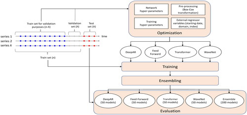
The overall pipeline considered for implementing the DL forecasting models of this study is summarized in Figure 1. The source code for the implementation is available at github.com/gjmulder/m3-gluonts-ensemble.

Figure 1. The pipeline considered for implementing the DL forecasting models of the present study. The models are optimized in terms of network hyper-parameters, training hyper-parameters, pre-processing, and external regressor variables simultaneously. The optimal parameters are then used for training multiple models of each type, resulting into various ensembles.

3. Forecasting the 1,045 longest monthly series of the M3 competition

In 2010, Ahmed et al. (2010) published a study that empirically compared the forecasting accuracy of eight ML forecasting methods, utilizing the 1,045 monthly series of the M3 competition (Makridakis & Hibon, 2000) containing more than 80 observations (training sample). The authors concluded that there are significant differences between the methods in terms of accuracy, with different pre-processing approaches having also different impact on their performance. Note, however, that the study of Ahmed et al. (2010) utilized only ML methods without comparing their accuracy to standard, statistical benchmarks.

To allow such comparisons, Makridakis et al. (2018) extended the study of Ahmed et al. (2010) in four directions. First, eight statistical methods were introduced as benchmarks to compare the accuracy of the ML methods considered. Second, two additional ML methods (Simple Recurrent Neural Network and Long Short Term Memory Neural Network) that had become popular during the last years were included in the study. Third, an additional accuracy measure (Mean Absolute Scaled Error – MASE; Hyndman & Koehler, 2006) was introduced in addition to the symmetric Mean Absolute Percentage Error (sMAPE) used by Ahmed et al. (2010) to make sure that similar conclusions would apply with a different evaluation measure (for more details, see Appendix B). Fourth, three different approaches were utilized for obtaining multi-step-ahead forecasts, thus enabling the evaluation of the ML methods considered for longer forecasting horizons and not just for one-step-ahead forecasts as it was done by Ahmed et al. (2010).

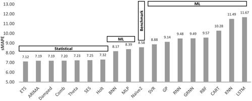
The results of the study of Makridakis et al. (2018) were surprising, indicating that the one-step-ahead forecasting accuracy of the best ML method (Bayesian Neural Network – BNN) was lower than that of the worst statistical one, being superior only to that of the Naive 2, a seasonally adjusted random-walk benchmark. Figure 2 presents the one-step-ahead forecasting accuracy (average of 18 one-step-ahead forecasts) of all the methods examined by Makridakis et al. (2018) in terms of sMAPE, highlighting the superiority of the statistical forecasting approaches. Similar conclusions were drawn for the case of the multi-step-ahead forecasts, where the best performing ML method managed to outperform only the Naive 2 benchmark in terms of sMAPE and the Naive 2, the Simple, and the Holt exponential smoothing (Gardner, 2006) in terms of MASE.

Figure 2. Forecasting accuracy (sMAPE) of the eight statistical and the ten ML forecasting methods examined by Makridakis et al. (2018). The results are reported for the 1,045 monthly series of the M3 competition containing more than 80 observations and refer to the average one-step-ahead forecasting accuracy of the methods, computed iteratively for the last 18 observations of the series.

In this section we expand the comparisons performed in Makridakis et al. (2018) to include DL methods using GluonTS, as described in Section 2. Note that in contrast to the local ML models considered by Makridakis et al. (2018), trained in a series-by-series fashion, the developed DL models are global, exploiting the benefits of cross-learning (Januschowski et al., 2020). Therefore, the aforementioned comparisons are effectively expanded to include global forecasting models as well.

In order to facilitate comparisons, instead of considering all the methods of Figure 2, we present Table 1 that lists the multi-step-ahead forecasting accuracy of the Naive 2 method, together with that of two popular statistical methods, i.e., ARIMA (Hyndman & Khandakar, 2008) and ETS (Hyndman et al., 2002), considered as standards for comparison, as well as the best performing ML methods (Multi-Layer Perceptron – MLP, and BNN) of Makridakis et al. (2018). In addition, we consider the simple combination (median) of the forecasts produced by ARIMA and ETS, to be called Ensemble-S. This ensemble, which involves the two most accurate statistical methods of Makridakis et al. (2018) and is similar to the simple statistical combination approach of Petropoulos and Svetunkov (2020), that has recently reported excellent results in the M4 competition, will serve as our primary benchmark. Finally, we report the corresponding forecasting accuracy of the four GluonTS models, as well as their ensemble (median), Ensemble-DL. The computational time (CT) of the methods, i.e., the time (measured in minutes) required by the methods for training and predicting all 1,045 series², as well as the relative computational complexity (RCC) of the methods, i.e., the number of floating point operations required by the methods for predicting all 1,045 series when compared to the Naive 2, is also reported. Note that Table 1 is similar to Tables A1 and A2 provided in Makridakis et al. (2018), with the addition of Ensemble-S, the four DL methods, and Ensemble-DL.

Table 1. The multi-step-ahead forecasting accuracy (sMAPE and MASE) of the top performing ML methods of the study of Makridakis et al. (2018), two statistical standards for comparison, their ensemble, and various DL models.

Method	Type	Number of models	sMAPE				MASE				CT	RCC
			Short	Medium	Long	Average	Short	Medium	Long	Average
Naive 2	Benchmark	1	10.75	12.38	15.01	12.71	0.75	1.04	1.35	1.05	1	1
ARIMA	Statistical	1	9.55	11.03	15.36	11.98	0.63	0.88	1.21	0.91	44	50
ETS	Statistical	1	9.09	10.68	13.72	11.17	0.63	0.89	1.19	0.90	34	38
Ensemble-S	Statistical	2	8.93	10.31	13.66	10.97	0.61	0.86	1.16	0.88	78	88
MLP	ML	100	9.53	12.34	15.00	12.29	0.66	0.98	1.24	0.96	83	166
BNN	ML	100	9.39	12.08	14.80	12.09	0.64	0.94	1.20	0.93	47	96
DeepAR	DL	50	9.23	10.91	13.60	11.25	0.65	0.90	1.23	0.93	9,064	313,000
Feed-Forward	DL	50	10.09	10.75	13.69	11.51	0.70	0.88	1.16	0.91	1,370	47,300
Transformer	DL	50	9.21	11.09	13.80	11.36	0.67	0.94	1.25	0.96	1,374	47,500
WaveNet	DL	50	10.41	10.66	13.45	11.51	0.80	0.92	1.19	0.97	8,872	306,000
Ensemble-DL	DL	200	8.83	9.90	12.50	10.41	0.62	0.83	1.12	0.86	20,680	713,800
Improvement of Ensemble-DL over Ensemble-S			0.10	0.41	1.16	0.56	−0.01	0.03	0.04	0.02
% Improvement of Ensemble-DL over Ensemble-S			1.1%	4.0%	8.5%	5.1%	−1.6%	3.5%	3.4%	2.3%

The results are reported for the 1,045 monthly series of the M3 competition containing more than 80 observations. The bold numbers highlight the best performing method per error measure and forecasting horizon. Short, medium, and long-term forecasts stand for 1–6, 7–12, and 13–18 month-ahead forecasts, respectively. The computational time (CT – measured in minutes) and the relative computational complexity (RCC) of the methods is also reported.

Table 2. The forecasting accuracy (sMAPE) of the top performing ML methods of the study of Makridakis et al. (2018), two statistical standards for comparison, their ensemble, and various DL models for different forecasting horizons.

Method	1	2	3	4	5	6	Avg. Short	8	12	Avg. Medium	15	18	Avg. Long
Naive 2	10.65	9.10	11.55	11.86	10.55	10.78	10.75	12.41	12.38	12.38	15.77	16.56	15.01
ARIMA	8.02	8.82	9.80	10.62	10.09	9.94	9.55	10.64	11.63	11.03	15.94	16.46	15.36
ETS	8.24	7.44	9.30	10.16	9.63	9.80	9.09	10.06	10.92	10.68	13.87	15.63	13.72
Ensemble-S	7.91	7.83	9.28	9.96	9.16	9.45	8.93	9.80	10.73	10.31	14.01	15.07	13.66
MLP	7.98	8.62	9.47	9.81	10.75	10.56	9.53	11.52	13.23	12.34	14.49	17.20	15.00
BNN	7.92	8.37	9.46	9.67	10.54	10.39	9.39	11.28	13.03	12.08	14.33	16.82	14.80
DeepAR	8.05	8.12	9.76	9.78	9.87	9.78	9.23	10.91	10.91	10.91	13.73	15.16	13.60
Feed-Forward	10.35	9.37	10.41	11.30	9.26	9.86	10.09	9.89	11.91	10.75	13.62	14.08	13.69
Transformer	8.86	8.28	9.15	9.92	9.02	10.02	9.21	11.17	11.12	11.09	13.81	15.68	13.80
WaveNet	10.06	9.53	11.51	12.11	9.38	9.87	10.41	10.08	11.20	10.66	13.87	14.50	13.45
Ensemble-DL	8.55	8.00	9.41	9.76	8.43	8.87	8.83	9.63	10.06	9.90	12.68	13.81	12.50
Improvement of Ensemble-DL
over Ensemble-S	−0.64	−0.17	−0.13	0.2	0.73	0.58	0.10	0.17	0.67	0.41	1.33	1.26	1.16
% Improvement of Ensemble-DL
over Ensemble-S	−8.1%	−2.2%	−1.4%	2.0%	8.0%	6.1%	1.1%	1.7%	6.2%	4.0%	9.5%	8.4%	8.5%

The results are reported for the 1,045 monthly series of the M3 competition containing more than 80 observations. The bold numbers highlight the best performing method per forecasting horizon. Short, medium, and long-term forecasts stand for 1–6, 7–12, and 13–18 month-ahead forecasts, respectively.

More specifically, Table 1 shows the sMAPE and MASE forecasting accuracy of the methods considered across the complete forecasting horizon (average of 18 forecasts), being also subdivided into the categories of short (1 to 6-step-ahead), medium (7 to 12-step-ahead), and long-term (13 to 18-step-ahead) forecasts. As seen, ETS and ARIMA are still more accurate on average than the ML methods and many of the individual DL methods according to sMAPE, both across all the forecasting horizons considered and their global average. Moreover, both Ensemble-S and Ensemble-DL are more accurate than the individual models that contribute to their construction. However, when compared to Ensemble-S, Ensemble-DL performs better in total. The same conclusions can be drawn according to MASE, with the exception of the short-term forecasts where Ensemble-S provides the best results. The forecasting accuracy of the DL ensemble is about 18% better than that of the Naive 2 method and around 5% and 2% than the statistical ensemble in terms of sMAPE and MASE, respectively. Note also that, in general, the improvements of Ensemble-DL over Ensemble-S are greater for medium and long-term forecasts. These results highlight the potential of DL, especially when multiple, diverse models are combined.

Combining has long been considered as an excellent alternative to single forecasting models, being one of the key finding of all the M competitions (Makridakis et al., 2020b). The most recent and indicative example is probably the study described in Petropoulos and Svetunkov (2020), that utilized a combination (median) of four relatively simple statistical methods for forecasting the M4 series, being ranked $6^{th}$ for the point forecasts (with a small difference compared to the second-best submission) and the respective 95% prediction intervals. Accordingly, ensembling has also been proven a powerful solution for the case of the ML methods, and particularly for NNs, with the median and the mode operators leading typically to better results (Kourentzes et al., 2014). The reasoning is two-fold: First, NNs are characterized by great variations when different initial parameter values are used, meaning that aggregating the results of multiple NNs instead of using a single one, enhances the robustness and the accuracy of the forecasts. Second, since each model is good at capturing different time series characteristics, combining their predictions allows for complex patterns to be effectively identified and then accurately extrapolated.

Note that similar results with those reported in Table 1 have been recently reported by Oreshkin et al. (2019), who utilized ensembles of multiple DL models to achieve more accurate forecasts than standard statistical methods in the M3 competition data. Interestingly, although the DL ensembles considered by Oreshkin et al. (2019) reported excellent forecasting performance, being significantly more accurate than the benchmarks, the individual DL models used for constructing the ensembles were relatively inaccurate. This finding is in line with our results, highlighting the value of combining various DL models, each considering different techniques for analysing and extrapolating time series patterns.

However, by examining Table 1, there is an issue that has to be further explored: Why do ARIMA, ETS and their ensemble, some relatively simple statistical methods, provide similarly accurate or even more accurate short-term forecasts than the DL models and their ensemble, but inferior results when medium or long-term forecasts are considered? In order to better investigate this issue, Table 2 disaggregates the results of Table 1 for the case of the sMAPE measure, reporting the forecasting accuracy of the statistical, ML, and DL methods considered across various forecasting horizons separately.

As seen, there is a clear ascending trend in regards to the forecast error across all statistical, ML, and DL methods considered. Long-term forecasts tend to be less accurate than the short-term ones, as expected. However, the forecasting accuracy at the earlier forecasting horizons and the rate at which it deteriorates for longer ones is different for different types of methods. This is demonstrated by the percentage improvements reported for each forecasting horizon for Ensemble-DL over Ensemble-S. Specifically, we find that Ensemble-DL is 8.1% less accurate in the first forecasting horizon compared to Ensemble-S, but after the fourth horizon it provides increasingly more accurate results, being 8.4% more accurate in the last forecasting horizon. A similar pattern emerges for the ML methods examined, i.e., MLP and BNN. In the first forecasting horizon they provide more accurate forecasts than those of the four DL methods and their ensemble. However, in the later horizons, they perform significantly worse.

In an attempt to explain the results of Table 2, we hypothesize that the differences reported in the relative performance of the examined models are directly linked to the learning objective that guides their optimization process. Specifically, our hypothesis is that when models are optimized based on their one-step-ahead forecasting accuracy, their forecasts will be relatively more accurate for short-term forecasts compared to models that are optimized based on their multi-step-ahead forecasting accuracy, and vice versa. Effectively, the overall accuracy of the former type of models will depend on the rate at which the one-step-ahead forecast errors accumulate recursively, while the overall accuracy of the latter type of models will be mostly driven by their ability to relate historical data with multiple forecasting horizons simultaneously. Drawing from the above, this hypothesis provides a reasonable explanation to our previous findings. Typically, statistical forecasting methods are optimized in terms of parameters so that the one-step-ahead forecast error is minimized. This is exactly the case for the statistical standards for comparison (ETS and ARIMA) considered in our study, that are parameterized with the objective to minimize the in-sample mean squared error of their forecasts. Similarly, the ML benchmarks of Makridakis et al. (2018) (MLP and BNN) have been parameterized with the objective to produce accurate multi-step-ahead forecasts in a recursive fashion. As a result, although these methods are highly accurate in the first few forecasting horizons, their relative forecasting performance deteriorates fast, in contrast to DL models that are optimized for multi-step-ahead forecasting and, therefore, are specialized for this particular forecasting task.

To empirically test our hypothesis, we conducted a simple experiment where we used the Holt exponential smoothing model (Gardner, 2006) to forecast the 1,045 monthly series of the M3 competition containing more than 80 observations, using two different approaches for optimizing the parameters of the model, i.e., the smoothing parameters that determine the level and trend components of the forecasts. In the first case, the parameters were optimized based on the one-step-ahead forecast error, as traditionally done by most forecasting software. In the second case, the model parameters were optimized based on the average error of the 18-step-ahead forecasts. After producing the forecasts, the relative forecasting accuracy of the first variant over the second was computed for each forecasting horizon, as shown in Figure 3. It can be seen that there is a clear descending trend in the relative accuracy of the two forecasting approaches. Although for short-term forecasts the first variant provides better results, these improvements are diminished for medium-term forecasts, becoming negative for long-term ones.

Figure 3. The relative forecasting accuracy (sMAPE) of the 18-step-ahead-optimized Holt method over the one-step-ahead-optimized Holt method. The results are reported for the 1,045 monthly series of the M3 competition containing more than 80 observations and for each forecasting horizon separately. Points that are below the red horizontal line indicate forecasting horizons where the 18-step-ahead variant provides more accurate forecasts than the one-step-ahead one, and vice versa.

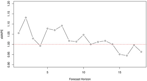
Overall, the theoretical explanation and the empirical results provided above support our initial hypothesis. Moreover, our findings are in line with those of past studies that have evaluated various strategies for training multi-step-ahead ML models, including the recursive, direct, and multi-input multi-output ones, among others (Ben Taieb et al., 2010, 2012). Therefore, we conclude that although statistical methods may provide more accurate short-term forecasts than DL methods, the latter can effectively balance learning across multiple forecasting horizons, sacrificing part of their short-term accuracy to ensure adequate performance in the long-term. Will this conclusion apply to other data sets beyond the 1,045 longest monthly series of the M3 competition? Is this the norm or an exception? The following section, where all 3,003 M3 data are considered to perform relative comparisons, sheds more light on these questions.

4. Forecasting all 3,003 series of the M3 competition

In this section, we extend the accuracy comparisons performed in the previous one to all 3,003 series of the M3 competition that involve yearly, quarterly, and “other” series along with the monthly ones. Moreover, we discuss the similarities and differences between the results of the two data sets and explore further the question on whether statistical models are more appropriate for short-term forecasting, with DL ones being more accurate for long-term predictions.

Table 3 summarizes the average forecasting accuracy of GluonTS models in terms of sMAPE for all 3,003 series of the M3 competition. Yearly data involve 645 series and 6-step-ahead forecasts, quarterly data 756 series and 8-step-ahead forecasts, monthly data 1,428 series and 18-step-ahead forecasts, while “other” data 174 series and 8-step-ahead forecasts. The average forecasting accuracy of the methods is computed as the global average of the 37,014 forecasts required by the organizers of the competition (number of series multiplied by the respective forecasting horizon). Moreover, a variety of forecasting methods originally submitted in the M3 competition are included as benchmarks along with the two standards for comparison, and some state-of-the-art statistical, ML, and DL methods that have been recently tested using all the 3,003 M3 data. Note that the accuracy of the benchmarks included in the original M3 study has been re-computed based on the error measure used in this paper. In this regard, the results presented in Table 3 are slightly different to those reported in Makridakis and Hibon (2000).

Table 3. The multi-step-ahead forecasting accuracy (sMAPE) of popular statistical and ML models compared with that of various DL ones.

			Yearly	Quarterly	Monthly	Other	Average
Method		Type	645	756	1,428	174	3,003
M3 competition study (Makridakis & Hibon, 2000)	Naive 2	Benchmark	17.88	9.95	16.89	6.30	15.46
	B’J automatic	Statistical	17.73	10.26	14.80	5.06	13.99
	Comb S-H-D	Statistical	17.07	9.22	14.47	4.56	13.51
	ForecastPro	Statistical	17.27	9.82	13.90	4.60	13.23
	Theta	Statistical	16.97	8.96	13.89	4.41	13.05
Standards for comparison	ARIMA (Hyndman & Khandakar, 2008)	Statistical	17.10	10.01	14.90	4.51	13.94
	ETS (Hyndman et al., 2002)	Statistical	17.00	9.68	14.14	4.37	13.34
	Ensemble-S	Statistical	16.49	9.50	13.83	4.37	13.04
	Global-LM	Statistical	16.72	17.52	17.57	4.78	16.99
Other M3 studies	DOTM (Fiorucci et al., 2016)	Statistical	15.94	9.28	13.74	4.58	12.90
	EXP (Spiliotis et al., 2019a)	Statistical	16.39	8.98	13.43	5.46	12.71
	LGT (Smyl & Kuber, 2016)	ML	15.23	n/a	n/a	4.26	n/a
	Bagged.BLD.MBB.ETS (Bergmeir et al., 2016)	Statistical	17.89	10.13	13.64	n/a	n/a
	Bagged.Cluster.ET (Dantas & Cyrino Oliveira, 2018)	Statistical	17.56	9.89	13.62	n/a	n/a
N-BEATS (Oreshkin et al., 2019)	N-BEATS-G	DL	16.20	8.92	13.19	4.19	12.47
	N-BEATS-I	DL	15.84	9.03	13.15	4.30	12.43
	N-BEATS-I + G	DL	15.93	8.84	13.11	4.24	12.37
GluonTS	DeepAR	DL	15.42	9.00	13.64	4.13	12.71
	Feed-Forward	DL	16.55	9.15	14.36	4.53	13.37
	Transformer	DL	16.38	9.23	14.45	4.41	13.42
	WaveNet	DL	18.36	13.62	13.84	5.53	13.96
	Ensemble-DL	DL	15.29	8.79	13.07	4.32	12.27
Improvement of Ensemble-DL over Ensemble-S			1.20	0.71	0.76	0.05	0.77
% Improvement of Ensemble-DL over Ensemble-S			7.3%	7.5%	5.5%	1.1%	5.9%

The results are reported for all the 3,003 series of the M3 competition, both per data frequency and total. The bold numbers highlight the best performing method per data frequency.

We expand the accuracy comparisons between DL and statistical forecasting approaches to account for statistical models trained in a cross-learning fashion. Although, traditionally, statistical models are fitted on the data of a single series and tasked with producing forecasts for that same series (local models), assessing the accuracy of their global counterparts would further improve the quality of the comparisons. Since most statistical models are not well-suited for cross-learning, we consider a linear regression model trained in a cross-learning fashion, to be called Global-LM, similar to that proposed by Montero-Manso and Hyndman (2021). For the different subsets of series, the number of past observations used by Global-LM to forecast the future ones is equal to the forecasting horizon, i.e., 6 for yearly series, 8 for quarterly series, 18 for monthly series, and 8 for “other” series. Global-LM is trained to produce one-step-ahead forecasts and, therefore, multiple-step-ahead forecasts are computed iteratively, i.e., by applying the recursive forecasting strategy (Ben Taieb et al., 2012).

Observe that Ensemble-DL continues to be the most accurate forecasting approach overall. This is true for all data frequencies, except of the yearly series where, by a small margin, the DL ensemble is outperformed by LGT, a ML forecasting method (Smyl & Kuber, 2016). From these findings, we can conclude that DL models are capable of providing accurate results overall and for various types of data (Spiliotis et al., 2020b). The GluonTS ensemble does not always outperform the individual DL models used for its construction, with DeepAR doing better in the data labelled as “other.” This could indicate that, although the ensembles of multiple DL models lead to more accurate results, depending on the particular characteristics of the series, other models could be more appropriate in different situations (Petropoulos et al., 2014) and various forecasting horizons.

We also observe that the improvements reported for the DL ensemble over the statistical ensemble are greater for lower frequency data, i.e., yearly and quarterly series. In particular, Ensemble-DL is 7.3% and 7.5% more accurate than Ensemble-S for the yearly and quarterly data respectively, and 5.5% better for the monthly series. This finding is in line with our “horses for courses” argument, suggesting that the improvements of DL methods may vary depending on the particularities of the series being predicted.

Interestingly, the accuracy of the Ensemble-DL and the N-BEATS (Oreshkin et al., 2019), another state-of-the-art DL forecasting approach, are very similar across all data frequencies, with the former being a little more accurate in all frequencies except that of “other” series. However, the differences between the two approaches are minimal, ranging from 0.64 (yearly data) to −0.08 (“other” data), with GluonTS having on average a slight advantage of 0.10 over N-BEATS. This finding could suggest that current DL approaches have similar learning capacities, leading to comparable results when ensembles of multiple DL models are considered.

Although the results of Table 3 suggest that Ensemble-DL is more accurate than Ensemble-S across all data frequencies, one could argue that part of the improvements may be attributed to the greater number of models Ensemble-DL (four models) uses over Ensemble-S (two models). To shed some light in this direction we combine the forecasts of the individual DL models in pairs and compute the accuracy of the resulting ensembles, as shown in Table 4. Overall, when all 3,003 series are taken into consideration, we observe that all pairwise DL combinations produce 0.4% to 6.1% more accurate forecasts than Ensemble-S. The same is true for the yearly and the monthly series where, with the exception of the “Feed-Forward & Transformer” ensemble in the monthly series, all pairwise ensembles improve on average accuracy by more than 4% over the Ensemble-S benchmark. Similar conclusions can be drawn for the quarterly and “other” data, although in this case “Feed-Forward & WaveNet” and “Transformer & WaveNet” do worse than Ensemble-S. Interestingly, ensembles that involve DeepAR, i.e., the most accurate individual DL model, consistently outperform the rest, while ensembles that involve WaveNet, i.e., the least accurate individual DL model, sometimes deteriorate forecasting performance. This finding suggests that ensembles that involve more skilful models are more likely to further improve forecasting performance. Nevertheless, we find that the accuracy of Ensemble-DL is comparable to that of the best pairwise ensemble, despite the fact it contains forecasts from less accurate DL models. Given that identifying a priory the most accurate base models to be used in an ensemble can be a challenging and time intensive process, it is encouraging to find that larger yet simple ensembles can effectively improve overall accuracy.

Table 4. The multi-step-ahead forecasting accuracy (sMAPE) of various DL models compared with that of their pairwise ensembles as well as Ensemble-DL (median of all four DL models) and Ensemble-S (median of two statistical models).

	Yearly	Quarterly	Monthly	Other	Average
Method	645	756	1,428	174	3,003
Ensemble-DL	15.29	8.79	13.07	4.32	12.27
Ensemble-S	16.49	9.50	13.83	4.37	13.04
DeepAR & Feed-Forward	15.24	8.73	13.07	4.16	12.25
DeepAR & Transformer	15.06	8.60	13.44	4.10	12.47
DeepAR & WaveNet	15.69	9.18	13.09	4.32	12.39
Feed-Forward & Transformer	15.74	8.78	13.85	4.36	12.86
Feed-Forward & WaveNet	16.39	10.20	13.56	4.76	12.98
Transformer & WaveNet	16.34	10.11	13.62	4.66	12.99

The results are reported for all the 3,003 series of the M3 competition, both per data frequency and total. The bold numbers highlight the best performing method per data frequency.

An interesting case in the results of Table 3 that requires further discussion is that of global statistical models. Global-LM ranks last among all methods considered by a large margin when tasked with forecasting quarterly and monthly series. However, it is a much more viable forecasting approach in the case of yearly and “other” series. This discrepancy can be attributed to the simplified assumptions that the linear regression model makes and the challenges of the examined forecasting task. The existence of seasonal patterns in quarterly and monthly time series along with the longer forecasting horizons make the task of effectively fitting a linear model for these series more difficult compared to the case of yearly data that are dominated by linear trends. Traditional, local statistical models can focus their modelling capacity on the particular patterns of each series and, therefore, outperform the single global one. Recall that, in contrast to Global-LM, some local models can effectively account for multiplicative trend and seasonality if needed, thus being more generic. On the other hand, DL approaches offer significantly more potent models that are able to effectively learn complex patterns from larger sets of series. As a result, Global-LM performs worse than all other classes of models, while global DL models, and especially their ensemble, provide the most accurate results overall.

Table 5 is similar to Table 3, but instead of examining the accuracy of the various forecasting methods across different data frequencies, the performance of the methods is reported for different forecasting horizons, as done in Table 2 for the case of the 1,045 longest monthly series of M3. For reasons of brevity, the results are summarized for all 3,003-time series of M3, rather than for each data frequency separately. Moreover, the forecasting methods included are those for which detailed forecasts were provided per forecasting horizon.

Table 5. The forecasting accuracy (sMAPE) of various statistical models compared with that of DL ones for different forecasting horizons.

Method		1	2	3	4	5	6	Avg. Short	8	12	Avg. Medium	15	18	Avg. Long
M3 competition study (Makridakis & Hibon, 2000)	Naive 2	10.45	11.33	13.63	15.06	15.06	15.76	13.55	14.51	15.99	15.58	19.32	20.70	19.58
	B’J automatic	9.19	10.40	12.22	13.87	14.03	14.63	12.39	13.00	14.06	13.57	17.76	19.26	18.01
	Comb S-H-D	8.87	10.01	12.04	13.46	13.67	14.04	12.02	12.41	13.63	13.15	17.28	18.26	17.22
	ForecastPro	8.61	9.57	11.44	13.01	13.43	14.26	11.72	12.67	13.31	13.06	16.43	18.29	16.73
	Theta	8.40	9.57	11.31	12.53	13.19	13.92	11.49	11.98	13.23	12.92	16.36	18.36	16.67
Standards for for comparison	ARIMA (Hyndman & Khandakar, 2008)	8.58	10.01	11.84	13.22	13.80	14.58	12.00	13.08	14.03	13.55	18.44	20.00	18.50
	ETS (Hyndman et al., 2002)	8.54	9.51	11.39	12.93	13.34	14.20	11.65	12.62	13.45	13.12	17.00	19.20	17.18
	Ensemble-S	8.35	9.49	11.27	12.68	12.94	13.85	11.43	12.35	13.05	12.75	16.74	18.31	16.80
	Global-LM	10.42	11.57	13.54	15.88	16.71	18.05	14.36	19.28	17.39	17.40	21.44	23.54	22.03
GluonTS	DeepAR	8.04	9.54	11.23	12.02	12.59	13.26	11.11	12.28	13.31	12.77	15.83	17.26	15.99
	Feed-Forward	9.44	10.25	11.82	13.05	12.86	14.25	11.95	12.07	14.34	12.98	16.68	17.39	16.82
	Transformer	9.25	10.07	11.68	12.72	12.80	13.99	11.75	12.58	13.75	13.32	16.77	18.17	17.05
	WaveNet	11.02	11.64	13.40	14.24	14.15	15.23	13.28	12.74	13.44	13.14	16.45	17.41	16.41
	Ensemble-DL	8.35	9.35	11.09	11.95	11.99	12.95	10.95	11.41	12.52	12.03	15.24	16.42	15.36
Improvement of Ensemble-DL over Ensemble-S		0.00	0.14	0.18	0.73	0.95	0.9	0.48	0.94	0.53	0.72	1.50	1.89	1.44
% Improvement of Ensemble-DL over Ensemble-S		0.0%	1.5%	1.6%	5.8%	7.3%	6.5%	4.2%	7.6%	4.1%	5.6%	9.0%	10.3%	8.6%

The results are reported for all the 3,003 series of the M3 competition. The bold numbers highlight the best performing method per forecasting horizon. Short, medium, and long-term forecasts stand for 1–6, 7–12, and 13–18 period-ahead forecasts, respectively.

Notice that, with the exception of DeepAR, the individual DL models are less accurate than the best performing statistical one for short and medium horizons, with the differences becoming smaller however as the forecasting horizon increases. In particular, Theta is more accurate than the Feed-Forward, Transformer, and WaveNet models for short (by 3.9%, 2.2%, and 13.5%, respectively) and medium-term forecasts (by 2.1%, 4.2%, and 2.2%, respectively). However, Theta outperforms only the Feed-Forward and Transformer model for long-term forecasts (by 0.9% and 2.2%, respectively), being also less accurate than the WaveNet model (by 1.6%). With the exception of the three shorter forecasting horizons, Global-LM provides the least accurate forecasts compared to the rest of the forecasting methods considered. Even when compared to the Naive 2 method, Global-LM is 6.0%, 11.7%, and 12.5% less accurate for short, medium, and long horizons, respectively.

The results of Table 5 reconfirm the power of combining. Both Ensemble-S and Ensemble-DL provided more accurate results than those of their constituent methods, although DeepAR is about 4% better for the case of the one-step-ahead forecasts. However, observe that in contrast to Table 2, where the ensemble of the statistical methods outperformed the DL ensemble for horizons 1, 2 and 3, Ensemble-DL is at least as accurate or superior to Ensemble-S when the complete M3 data set is considered, across all horizons.

Both Tables 3 and 5 indicate that DL methods can lead to greater accuracy improvements, compared to their statistical counterparts, when tasked with forecasting yearly or quarterly series. This becomes evident not only by examining the per-frequency summary results of Table 3, but also by comparing the per-horizon results of Table 5 to those of Table 2. In the case of Table 2, where only 1,045 monthly series are considered, the percentage improvement of Ensemble-DL over Ensemble-S for the first 6 forecasting horizons ranges from −8.1% to 6.1%, with statistical methods being clearly superior to DL for horizons 1, 2, and 3. In the case of Table 5, the results for the first 6 horizons summarize the errors from yearly, quarterly, monthly, and “other” series (accounting for 21%, 25%, 48% and 6% of the 3,003 forecasts respectively). As a result, due to the improved performance of DL methods in forecasting lower frequency series, the corresponding percentage improvement, across all 3,003 series, ranges from 0.0% to 6.5%, with DL methods outperforming statistical standards for comparisons across all horizons.

Returning to the initial question on whether statistical models, optimized for one-step-ahead forecasts, are more appropriate for short-term forecasting, the results reported in the present section indicate that, when all 3,003 series are considered, although DL methods perform better overall, their advantage is still limited in the early forecasting horizons and increases for medium and long term forecasts. Thus, it is safe to conclude that the hypothesis presented in Section 3 holds true for the expanded set of series.

However, even though it is apparent in both Tables 2 and 5 that a clear pattern exists, regarding the improvement of Ensemble-DL over Ensemble-S, it is still unclear why for the case of 1,045 monthly series the improvements range from −8.1% to 9.5%, while for the case of all 3,003 series range from 0.0% to 10.3%. The answer to this question may lie in the size of the forecasting horizon used when forecasting series of different frequencies, that is set to 6 for yearly forecasts, 8 for quarterly and other forecasts, and 18 for monthly forecasts. DL methods optimized for multi-step-ahead forecasts, despite their significant learning capacity, are forced to split their “attention” in order to provide reasonable forecasts for the entire horizon. Essentially, only a fraction of their strength is dedicated to any single point of the horizon. Naturally, as the length of the horizon increases, the importance of each individual forecast is reduced and the short-term forecasting performance of multi-step-ahead methods will decrease, and vice versa. On the other hand, statistical methods optimized for one-step-ahead forecasts dedicate their full potential on extrapolating the series one step into the future, irrespective of the length of the horizon. As a result, the improved relative performance of DL methods in the first forecasting horizons is to be expected when series with shorter horizons are included, compared to when only series that require 18-step-ahead forecasts are considered.

In order to investigate the differences reported between the DL methods over the standards for comparison, and especially Ensemble-S, we employ the multiple comparisons with the best (MCB) test (Koning et al., 2005). The test computes the average ranks of the forecasting methods according to sMAPE across the complete data set of the M3 competition and concludes whether or not these are statistically different. Figure 4 presents the results of the analysis. If the intervals of two methods do not overlap, this indicates a statistically different performance. Thus, methods that do not overlap with the grey interval of the figure are considered significantly worse than the best, and vice versa.

Figure 4. Average ranks and 95% confidence intervals of the standards for comparison and the DL forecasting methods, as well as the global linear model, over all the 3,003 series of the M3 competition: multiple comparisons with the best (sMAPE used for ranking the methods) as proposed by Koning et al. (2005).

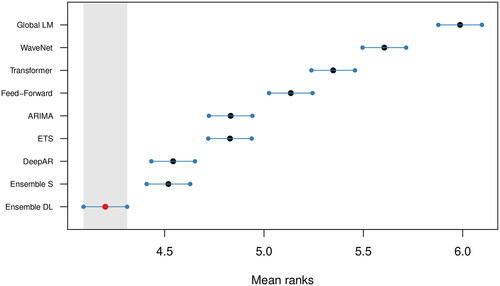
According to MCB, we find that Ensemble-DL is significantly more accurate than the rest of the forecasting methods considered in this study, including the DL models it consists of. On a second level, Ensemble-S provides significantly more accurate forecasts than the contributing ETS and ARIMA models. Overall, the power of ensembling is once again confirmed. Finally, despite the dominance of Ensemble-DL, only DeepAR, among all individual DL methods, produces significantly more accurate forecasts than those of the top-performing statistical methods.

Although the results of the MCB test clearly support the superiority of Ensemble-DL, both over the individual DL models and the examined statistical ensemble, using a larger sample of forecasts to conduct comparisons would have allowed for better generalization of our findings. In this regard, we consider the rolling origin evaluation approach (Tashman, 2000) which is equivalent to cross-validation for time series data. According to this approach, a period of historical data is first used for training the examined forecasting methods. Then, the methods are used to produce forecasts for a given forecasting horizon and the accuracy is measured based on the actual values of the series in the corresponding test period. Subsequently, the forecast origin is shifted, the methods are re-trained using the new data that have become available, and new forecasts are produced, contributing another evaluation. This process is repeated till there are no data left for testing and the overall performance of the methods is determined based on their average accuracy over the conducted evaluations. In our case, and given that DL models are particularly computationally expensive to run for multiple forecast origins, we applied the described evaluation scheme over the complete M3 data set for two consecutive origins using a shifting step that was equal to the forecasting horizon so that the two test sets do not overlap.

Table 6 summarizes the results of the rolling origin evaluation for the statistical and the DL ensemble, as well as of the individual models involved in these combinations. As seen, the results are very similar to those reported in Table 3, both across all series and per data frequency, confirming our previous findings. The consistency of our results can be justified by the high representativeness of the M3 data set. The M3 time series have different starting points and lengths. As a result, the out-of-sample period used for evaluating the forecasts will effectively differ among the series, meaning that the dominance of one forecasting method over the others is unlikely to be attributed to a specific forecast origin, economic cycle, or seasonal pattern that would favour its use.

Table 6. The multi-step-ahead forecasting accuracy (sMAPE) of the examined DL models compared with that of the standards for comparison and their ensembles considering a rolling origin evaluation approach.

	Yearly	Quarterly	Monthly	Other	Average
Method	645	756	1,428	174	3,003
ARIMA	18.38	9.95	15.12	4.22	14.21
ETS	19.27	9.43	14.88	4.22	14.04
Ensemble-S	18.13	9.38	14.28	4.13	13.50
DeepAR	17.27	8.96	13.84	3.99	13.03
Feed-Forward	18.12	9.06	14.79	4.37	13.81
Transformer	18.02	9.18	14.74	4.17	13.78
WaveNet	20.47	13.48	13.98	5.17	14.24
Ensemble-DL	16.93	8.72	13.32	4.11	12.60

The results are reported for all the 3,003 series of the M3 competition, both per data frequency and total. The bold numbers highlight the best performing method per data frequency.

5. DL methods: Advantages and drawbacks

Selecting and optimizing the most accurate forecasting model has fundamentally changed over the last 60 years. In his excellent paper “A brief history of forecasting competitions,” Hyndman (2020) quotes the comments made by two discussants of the Makridakis et al. (1979) study to illustrate the thinking of the time (Makridakis et al., 1979). The first discussant commented “The combined forecasting methods seem to me to be non-starters… Is a combined method not in danger of falling between two stools?,” while the second added “The authors’ suggestion about combining different forecasts is an interesting one, but its validity would seem to depend on the assumption that the model used in the Box-Jenkins approach is inadequate – for otherwise, the Box-Jenkins forecast alone would be optimal.”

Hyndman continues his review with what can be described as the dominant approach of that time that required identifying judgmentally the most appropriate model for each time series, suggesting that way a strong bias against automatic forecasting procedures, as expressed by Jenkins: “The fact remains that model building is best done by the human brain and is inevitably an iterative process.”

Gradually, combining the forecasts of more than one methods was accepted as a useful alternative to using a single one (Claeskens et al., 2016) while automatic selection of the most appropriate model became a common practice (Fildes & Petropoulos, 2015; Spiliotis et al., 2020a). Yet, combining and automatic model selection are just two parts of how DL models work nowadays. All four of the GluonTS and the two N-BEATS forecasting models have two main things in common. First, the forecasts are produced without specifying an underlying data generating process (e.g., in terms of trend and seasonality). The users do determine the hyper-parameters of the models to facilitate training, but after specifying these values, data relationships are found in an automatic way without making any assumptions about the data patterns. The optimization of the NN weights, which are responsible for deriving the final forecasts, is done starting with some initial values that are improved with each additional iteration in order to arrive at an “optimal” model. Second, a large number of such models are used in an ensemble to provide more robust and accurate performance. Overall, state-of-the-art DL models can be effectively trained in order to become accurate forecasting tools, and, when several models are combined, further accuracy improvements are to be expected. On the other hand, the construction of accurate DL forecasting models is more like an art, depending heavily on the skills, the experience, and the background of the forecaster, meaning human brain and judgment are still relevant for building accurate models (Barker, 2020). However, once the hyper-parameters have been set, forecasting using DL becomes rather automated.

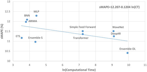
The results of this study highlight the potential of DL methods for time series forecasting applications, indicating that sophisticated models are able to provide more accurate results than their statistical and ML counterparts, especially when ensembles of multiple models are used. However, even in the Big Data era, computation time is still important, especially in settings where getting fast results is equally or even more important than getting accurate forecasts (Nikolopoulos & Petropoulos, 2018). In certain applications, “pre-trained” models can be employed without additional training and, as a result, the cost of using DL methods can be reduced. However, in many cases, model training cannot be avoided and practitioners are required to train new models or re-train old ones. The computational time reported in this study includes the time required for both training the models and producing the requested forecasts, with training time constituting the majority of it. Figure 5 visualizes the trade-off between optimal versus sub-optimal solutions in terms of forecasting performance versus computational time for the case of the 1,045 longest monthly series of M3. As seen, the additional cost that has to be paid for using a DL model in order to improve forecasting accuracy to a small extent is extensive. In particular, it is shown that a drop of 10% in terms of forecasting error could require an additional computational time of about 15 days, which if not decreased, e.g., by using more and faster processors in parallel, is probably prohibiting the utilization of advanced DL approaches for every day forecasting tasks that require training new models (or re-training old ones). In this regard, it becomes evident that, for practical reasons, if DL methods are to be widely adopted by business firms and other organizations, their computational requirements must be reduced considerably. Otherwise, traditional, statistical methods and standard ML ones of lower computational requirements will continue to dominate the field of forecasting.

Figure 5. Forecasting performance (sMAPE) versus computational time (CT). The results are reported for multi-step-ahead forecasts for the 1,045 monthly series of M3 containing more than 80 observations. An ln(CT) of zero corresponds to about 1 min of computational time, while an ln(CT) of 2, 4, 6, 8, and 10 correspond to about 7 min, 1 h, 7 h, 2 days, and 15 days, respectively.

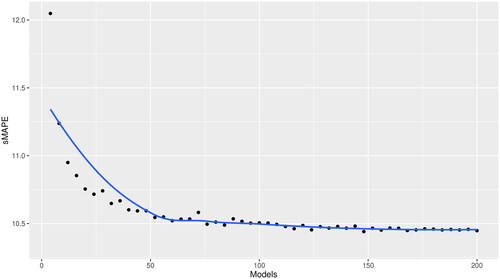
In an attempt to reduce the overall computational cost of the examined DL approaches and make them more efficient, we question the importance of considering numerous DL models within the ensemble. Figure 6 shows the sMAPE of the multi-step-ahead forecasts produced by various ensembles of GluonTS models (DeepAR, Feed-Forward, Transformer, and WaveNet) for the case of the 1,045 longest monthly series of M3. Observe that, as the number of the DL models used in the ensemble increases, the accuracy is improved, first at a steep rate and then at a smaller pace. However, it seems that a number of about 75 models may be enough for producing results whose accuracy is similar to those reported for the 200 models with about one third of the computational cost. This suggests that the efficiency of DL forecasting approaches can be significantly improved without a major impact on their accuracy if their computationally-intensive processes are restricted to a reasonable number of models. At the same time, as computer power is increasing and programming is becoming more efficient, such costs could become less important in the future, thus allowing the wider utilization of DL.

Figure 6. Forecasting performance (sMAPE) of various ensembles of DL models. The results are reported for multi-step-ahead forecasts for the 1,045 monthly series of M3 containing more than 80 observations. For each ensemble, random combinations of the 50 DeepAR, Feed-Forward, Transformer, and WaveNet models were considered.

In summary, we find out that DL models produce more accurate forecasts than statistical and ML ones, especially for longer forecasting horizons. Ensembles of multiple models can be utilized to further improve performance, although at much greater computational cost. On the negative side, in most of the cases the overall forecasting procedure is a black-box, with the models being estimated mechanically in an automatic way. In this regard, although the forecasts derived by DL models could be superior to those of their statistical and ML counterparts, there is no direct way for a forecasting user to understand how the forecasts were made or how they would have been different if some factor would have changed.

As a final step in our analysis, we investigate how key time series features influence the forecasting accuracy of statistical and DL ensembles. This is because the literature suggests that different types of methods may be more appropriate for forecasting series of different characteristics (Petropoulos et al., 2014), meaning that DL approaches may perform better on average than statistical ones due to their ability to better handle particular patterns of data. To do so, similarly to Spiliotis et al. (2020b) we use a multiple linear regression (MLR) model to correlate the sMAPE value achieved by each ensemble for each time series in the M3 data set with the five intuitive time series features proposed by Kang et al. (2017), as follows: $$\mathit{sMAP}{E}_i=a{F}_{1_i}+b{F}_{2_i}+c{F}_{3_i}+d{F}_{4_i}+e{F}_{5_i},$$ where sMAPE_i is the error reported for the ith time series of the data set for Ensemble-S or Ensemble-DL. $F_{1_i}$ corresponds to the spectral entropy of series i, measuring its “forecastability” (or randomness), $F_{2_i}$ to its strength of trend, measuring long-term changes in its mean level, $F_{3_i}$ to its strength of seasonality, measuring the influence of the seasonal factors, $F_{4_i}$ to its first order autocorrelation, measuring the linear relationship between its observations, and $F_{5_i}$ to its optimal Box–Cox transformation parameter, measuring stability.

Before estimating the MLR models, both dependent (sMAPE) and independent (features) variables are scaled within the range of [0,1] so that the results are scale independent and easier to interpret. This allows us to detect features that explain the sMAPE variances and approximate their negative or positive effects on the forecasting accuracy. By comparing the coefficients of the individual MLR models we can then understand the strengths and weaknesses of each forecasting approach better; smaller coefficients suggest better accuracy and vice versa. The results are presented in Table 7. As can be seen, Ensemble-DL is generally more effective in handling noisy and trended series, in contrast to Ensemble-S that provides more accurate forecasts for seasonal data, as well as for series that are stable or linear. This finding is in line with the results of Table 3 where Ensemble-DL was found to be more accurate for predicting yearly and quarterly data, typically dominated by the trend component. Accordingly, the improvements of Ensemble-DL in the monthly series are smaller since, although DL models are more robust to randomness, the corresponding series are characterized by seasonality, a component which is modelled more effectively by statistical methods (Smyl, 2020).

Table 7. Coefficients of the MLR models relating the sMAPE values generated by the statistical and DL ensembles in the 3,003 series of the M3 competition with their features.

Method	Forecastability	Trend	Seasonality	Linearity	Stability	R^2
Ensemble-S	0.212	−0.011	−0.025	0.005	−0.022	0.523
Ensemble-DL	0.195	−0.013	−0.018	0.009	−0.020	0.532

The R² values of the MLR models are reported to quantify the interpretability of the results. The bold numbers highlight the enemble model that is expected to result in lower forecast error per time series feature. 

6. Conclusions

The forecasting spring started with the M4 competition when for the first time after close to 40 years a number of sophisticated ML methods were found to produce more accurate forecasts than simple, statistical ones. Research around the use of ML algorithms in forecasting has increased significantly since. More recently, DL models have been introduced (Oreshkin et al., 2019; Salinas et al., 2020) and captured the attention of academics and practitioners. The results of the present study further motivate research that will hopefully translate the recent advances of DL algorithms into greater forecasting accuracy improvements.

If we were asked to indicate the most substantial finding from the time series forecasting competitions so far, it would definitely be the value of combining. Such value has been confirmed in all M competitions, Kaggle competitions (Bojer & Meldgaard, 2021), as well as in numerous other studies, highlighting the potential value of ML and DL ensembles, among others. It is now practically certain that the old notion of an “optimal” model does not hold and that combining more than a single model cancels the errors and improves forecasting accuracy. An interesting variation of combining has been the development of hybrid methods, like the one introduced by Smyl (2020) that blended statistical and ML features to provide more accurate results while not increasing the computational costs significantly. Another, interesting possibility is the approach used by the runner up of the M4 competition that instead of arbitrarily combining forecasting methods, it devised a way to determine the optimal combination weights based on the features that the series displayed (Montero-Manso et al., 2020). Theoretically, if some better way than using the median or average of multiple forecasting models could be found, the accuracy improvements could be substantial. Additionally, hybrid approaches and optimal weighting schemes could break, at least partially, the black-box nature of the DL models by providing some ability to explain how the forecasts are made. Developing interpretable DL architectures, would be another promising alternative to break the black-box (Oreshkin et al., 2019).

In this study, the improvements reported for the DL ensemble over standard, statistical and ML methods are ranging to around 6% for the case of the 3,003 time series of the M3 competition. Although these results are indicative and should therefore be reconfirmed for other, larger data sets, as well as for other types of DL models, they demonstrate that the improvements achieved come at a considerable greater computational cost. GluonTS is one of the first publicly available packages that supports the development and utilization of state-of-the-art DL models. Clearly, other packages should become available in the future to enable forecasters to experiment with alternative DL tools, such as Google’s AutoML that is being adapted to handle time series forecasting problems. Equally important, the efficiency of the DL models should be further improved to make them computationally more competitive to their statistical and ML counterparts.

It is evident that one of the major limitations of DL relates to the time required for training them. Many practitioners and organisations do not have access to hardware that would make the use of DL models practical for them. Although it is possible to reduce the computational cost of forecasting with DL models by using pre-trained variants, such an approach has its shortcomings, which cannot be ignored in certain cases. Models that are trained in different sets of series than the ones they are tasked with predicting are likely to be less effective in capturing the specific characteristics of the target set. In the case of training models once in order to use them continuously in the future, models will become obsolete at some point and will not be able to capture new dynamics in the data. Thus, we believe that exploring the use of transfer-learning techniques, in the context of time series forecasting, is critical and could greatly boost the adoption of DL by practitioners and companies.

Another potentially beneficial approach could be combining statistical or ML models with DL ones depending on the time horizon of forecasting. As this study has found, statistical models are better suited for short-term forecasts, while DL ones are better in capturing the long-term characteristics of the data. Similarly, different models could be used based on the particular characteristics of the series, their frequency, and length. For instance, our results suggest that some ML models, like LGT (Smyl & Kuber, 2016), are still more accurate than DL ones for predicting yearly data, in contrast to quarterly and monthly series where the latter are superior. Thus, it could be the case that long, high-frequency (e.g., hourly and daily) series that display non-linear, complicated patterns could be better forecast using DL approaches. We believe that as the usage of DL increases and more experience is gained, additional findings will be discovered to further improve overall forecasting accuracy.

Finally, we should note that, although considerable work has been made towards improving point forecast accuracy, not much has been done to estimate correctly the uncertainty around these forecasts. This is also the case for the present study which focused on point estimated and did not investigate the performance of DL models in probabilistic settings. Thus, future research should focus on the investigation of the potential of DL approaches for correctly estimating probabilistic forecasts, offering some breakthroughs in the field of estimating uncertainty and continuing the forecasting spring. The most recent M competition, M5, which required the prediction of nine different quantiles to estimate the distributions of the hierarchical unit sales of Walmart, provides empirical evidence in that direction (Makridakis et al., 2020d).

Disclosure statement

No potential conflict of interest was reported by the authors.

Additional information

Funding

We are grateful to Amazon for supporting this work through the AWS Machine Learning Research Awards program. The resources provided were critical for conducting this study.

Notes

1 Although some ML models may assume particular types of data distributions, they usually make no assumptions in terms of time series patterns, including trend, seasonality, and data correlations, among others.

2 The time needed for determining the optimal hyper-parameter values for each DL method is not included in the CT reported in Table 1. That is because it is largely affected by the experimental setup (e.g. in terms of number of hyper-parameters being optimized and trials performed to determine the optimal set of hyper-parameters) and the experience of the developers, thus not being an inherent property of the specific method. However, regarding the present study, the time spent for tuning the four DL methods was 3,193, 512, 507 and 3,077 hours for DeepAR, Feed-Forward, Transformer, and WaveNet, respectively.

Appendix A.

Hyper-parameter values used for the DL models

This appendix presents the optimal hyper-parameter values that were used to build the DL models of this study. The values were determined for each data frequency (yearly, quarterly, monthly, and “other” series) separately. All values were determined automatically using the Tree-of-Parzen-Estimators (TPE) algorithm on a validation set, as described in Section 2. In that same section, a brief explanation of the hyper-parameters considered is also provided.

Table A1. The network and the training hyper-parameter values of the DeepAR model used in this study.

Hyper-parameter	Yearly	Quarterly	Monthly	Other
Network hyper-parameters
cell_type	LSTM	LSTM	LSTM	LSTM
num_layers	4	4	3	2
num_cells	512	256	512	512
dropout_rate	0.012	0.015	0.071	0.018
external regressor variables	False	False	True	True
Training hyper-parameters
epochs	128	512	128	256
num_batches_per_epoch	128	256	256	128
batch_size	128	64	32	128
patience	8	32	8	8
learning_rate	0.0025	0.0035	0.0025	0.0037
learning_rate_decay_factor	0.23	0.57	0.17	0.16
minimum_learning_rate	$1.7e^{-5}$	$2.5e^{-5}$	$3.2e^{-5}$	$5.7e^{-6}$
weight_decay	$2.4e^{-8}$	$5.2e^{-8}$	$1.5e^{-8}$	$7.4e^{-9}$
Box-Cox transformation	False	False	False	False

The optimal values were determined for each data frequency separately.

Table A2. The network and the training hyper-parameter values for the simple Feed-Forward model used in this study.

Hyper-parameter	Yearly	Quarterly	Monthly	Other
Network hyper-parameters
num_hidden_dimensions	[64, 32, 16]	[128, 64, 32]	[64, 32, 16]	[64, 32]
Training hyper-parameters
epochs	512	512	1024	256
num_batches_per_epoch	256	256	128	64
batch_size	64	64	128	64
patience	16	16	16	8
learning_rate	0.0022	0.0019	0.0012	0.002
learning_rate_decay_factor	0.57	0.74	0.62	0.19
minimum_learning_rate	$1.0e^{-5}$	$9.7e^{-6}$	$5.5e^{-5}$	$9.9e^{-5}$
weight_decay	$1.0e^{-9}$	$1.1e^{-9}$	$5.3e^{-8}$	$1.0e^{-8}$
Box-Cox transformation	False	False	False	False

The optimal values were determined for each data frequency separately.

Table A3. The network and the training hyper-parameter values for the Transformer model used in this study.

Hyper-parameter	Yearly	Quarterly	Monthly	Other
Network hyper-parameters
model_dim	8	64	32	64
num_heads	8	8	4	2
inner_ff_dim_scale	2	4	2	2
pre_seq	dn	d	dn	n
post_seq	ndr	nr	ndr	r
act_type	softrelu	softsign	relu	softrelu
dropout_rate	0.019	0.012	0.117	0.018
external regressor variables	True	True	True	True
Training hyper-parameters
epochs	256	256	1024	128
num_batches_per_epoch	128	256	32	256
batch_size	64	32	32	128
patience	16	32	64	8
learning_rate	0.0021	0.0031	0.0012	0.0019
learning_rate_decay_factor	0.19	0.38	0.47	0.65
minimum_learning_rate	$8.2e^{-5}$	$1.1e^{-5}$	$7.1e^{-6}$	$5.5e^{-6}$
weight_decay	$1.3e^{-9}$	$1.7e^{-9}$	$6.6e^{-9}$	$1.4e^{-8}$
Box-Cox transformation	False	False	False	False

The optimal values were determined for each data frequency separately. For the sequence of processing operations, the “r” stands for residual connections, “n” for normalization, and “d” for dropout.

Table A4. The network and the training hyper-parameter values for the WaveNet model used in this study.

Hyper-parameter	Yearly	Quarterly	Monthly	Other
Network hyper-parameters
embedding_dimension	16	64	16	16
num_bins	512	2048	512	2048
n_residue	26	26	25	22
n_skip	128	32	64	16
dilation_depth	2	2	3	2
n_stacks	1	2	2	2
act_type	softsign	relu	sigmoid	relu
Training hyper-parameters
epochs	512	256	512	512
num_batches_per_epoch	32	64	256	256
batch_size	128	128	256	32
patience	8	16	16	16
learning_rate	0.0018	0.0005	0.0008	0.0009
learning_rate_decay_factor	0.68	0.66	0.21	0.13
minimum_learning_rate	$9.3e^{-5}$	$6.5e^{-5}$	$1.0e^{-5}$	$5.4e^{-6}$
weight_decay	$6.6e^{-8}$	$1.5e^{-8}$	$1.6e^{-8}$	$1.2e^{-9}$
Box-Cox transformation	False	False	False	False

The optimal values were determined for each data frequency separately.

Appendix B.

Accuracy measures used

The accuracy of the forecasting methods considered in this study is compared using the symmetric mean absolute percentage error (sMAPE) (Makridakis, 1993) and the mean absolute scaled error (MASE) (Hyndman & Koehler, 2006). Both accuracy measures are used in the original study of Makridakis et al. (2018), as well as, in several other published studies utilizing the M3 competition’s data set. As a result, in order to be able to draw comparisons between the forecasting performance of the DL methods presented in this article and that of methods included in other studies, the same accuracy measures had to be used. The two accuracy measures are defined as follows: (B.1) $$\mathit{sMAPE}=\frac{2}{h}\sum _{t=n+1}^{n+h}\frac{\left|y_t-f_t\right|}{\left|y_t\right|+\left|f_t\right|}*100\%,$$(B.1) (B.2) $$\mathit{MASE}=\frac{\frac{1}{h}\sum _{t=n+1}^{n+h}\left|y_t-f_t\right|}{\frac{1}{n-m}\sum _{t=m+1}^n\left|y_t-y_{t-m}\right|,}$$(B.2) where f_t is the forecast of the method at point t, y_t the corresponding actual value of the series, h the forecasting horizon, n the number historical observations, and m the frequency of the series, i.e., 12 for monthly data. For more details about the measures, see Makridakis et al. (2020b).

References

- Abadi, M., Barham, P., Chen, J., Chen, Z., Davis, A., Dean, J., Devin, M., Ghemawat, S., Irving, G., Isard, M., Kudlur, M., Levenberg, J., Monga, R., Moore, S., Murray, D. G., Steiner, B., Tucker, P., Vasudevan, V., Warden, P., … Zheng, X. (2016). Tensorflow: A system for large-scale machine learning. In 12th USENIX Symposium on Operating Systems Design and Implementation (OSDI 16) (pp. 265–283). USENIX Association.
- Adya, M., & Collopy, F. (1998). How effective are neural networks at forecasting and prediction? A review and evaluation. Journal of Forecasting, 17(5–6), 481–495. https://doi.org/10.1002/(SICI)1099-131X(1998090)17:5/6<481::AID-FOR709>3.0.CO;2-Q
- Ahmed, N. K., Atiya, A. F., Gayar, N. E., & El-Shishiny, H. (2010). An empirical comparison of machine learning models for time series forecasting. Econometric Reviews, 29(5-6), 594–621. https://doi.org/10.1080/07474938.2010.481556
- Alexandrov, A., Benidis, K., Bohlke-Schneider, M., Flunkert, V., Gasthaus, J., Januschowski, T., Maddix, D. C., Rangapuram, S. S., Salinas, D., Schulz, J., Stella, L., Türkmen, A. C., & Wang, Y. (2019). Gluonts: Probabilistic time series models in python. CoRR, abs/1906.05264.
- Bandara, K., Bergmeir, C., & Smyl, S. (2020). Forecasting across time series databases using recurrent neural networks on groups of similar series: A clustering approach. Expert Systems with Applications, 140, 112896. https://doi.org/10.1016/j.eswa.2019.112896
- Barker, J. (2020). Machine learning in m4: What makes a good unstructured model? International Journal of Forecasting, 36(1), 150–155. https://doi.org/10.1016/j.ijforecast.2019.06.001
- Ben Taieb, S., Bontempi, G., Atiya, A. F., & Sorjamaa, A. (2012). A review and comparison of strategies for multi-step ahead time series forecasting based on the nn5 forecasting competition. Expert Systems with Applications, 39(8), 7067–7083. https://doi.org/10.1016/j.eswa.2012.01.039
- Ben Taieb, S., Sorjamaa, A., Bontempi, G. (2010). Multiple-output modelling for multi-step-ahead time series forecasting. (Subspace Learning/Selected Papers from the European Symposium on Time Series Prediction). Neurocomputing, 73, 1950–1957.
- Bergmeir, C., Hyndman, R. J., & Benítez, J. M. (2016). Bagging exponential smoothing methods using stl decomposition and box–cox transformation. International Journal of Forecasting, 32(2), 303–312. https://doi.org/10.1016/j.ijforecast.2015.07.002
- Bergstra, J. S., Bardenet, R., Bengio, Y., & Kégl, B. (2011). Algorithms for hyper-parameter optimization. In Advances in neural information processing systems (pp. 2546–2554).
- Bergstra, J., Komer, B., Eliasmith, C., Yamins, D., & Cox, D. (2015). Hyperopt: A python library for model selection and hyperparameter optimization. Computational Science & Discovery, 8(1), 014008. https://doi.org/10.1088/1749-4699/8/1/014008
- Bojer, C. S., & Meldgaard, J. P. (2021). Kaggle forecasting competitions: An overlooked learning opportunity. International Journal of Forecasting, 37(2), 587–603. https://doi.org/10.1016/j.ijforecast.2020.07.007
- Box, G., & Jenkins, G. (1970). Time series analysis: Forecasting and control. Holden-Day.
- Chae, Y. T., Horesh, R., Hwang, Y., & Lee, Y. M. (2016). Artificial neural network model for forecasting sub-hourly electricity usage in commercial buildings. Energy and Buildings, 111, 184–194. https://doi.org/10.1016/j.enbuild.2015.11.045
- Chatfield, C. (1993). Neural networks: Forecasting breakthrough or passing fad? International Journal of Forecasting, 9(1), 1–3. https://doi.org/10.1016/0169-2070(93)90043-M
- Claeskens, G., Magnus, J. R., Vasnev, A. L., & Wang, W. (2016). The forecast combination puzzle: A simple theoretical explanation. International Journal of Forecasting, 32(3), 754–762. https://doi.org/10.1016/j.ijforecast.2015.12.005
- Crone, S. F., Hibon, M., & Nikolopoulos, K. (2011). Advances in forecasting with neural networks? Empirical evidence from the NN3 competition on time series prediction. International Journal of Forecasting, 27(3), 635–660. https://doi.org/10.1016/j.ijforecast.2011.04.001
- Dantas, T. M., & Cyrino Oliveira, F. L. (2018). Improving time series forecasting: An approach combining bootstrap aggregation, clusters and exponential smoothing. International Journal of Forecasting, 34(4), 748–761. https://doi.org/10.1016/j.ijforecast.2018.05.006
- Dekker, M., van Donselaar, K., & Ouwehand, P. (2004). How to use aggregation and combined forecasting to improve seasonal demand forecasts. International Journal of Production Economics, 90(2), 151–167. https://doi.org/10.1016/j.ijpe.2004.02.004
- Deng, L. (2014). A tutorial survey of architectures, algorithms, and applications for deep learning – Erratum. APSIPA Transactions on Signal and Information Processing, 3(1), 1-29. https://doi.org/10.1017/ATSIP.2013.9
- Faust, O., Hagiwara, Y., Hong, T. J., Lih, O. S., & Acharya, U. R. (2018). Deep learning for healthcare applications based on physiological signals: A review. Computer Methods and Programs in Biomedicine, 161, 1–13.
- Fildes, R., & Petropoulos, F. (2015). Simple versus complex selection rules for forecasting many time series. Journal of Business Research, 68(8), 1692–1701. https://doi.org/10.1016/j.jbusres.2015.03.028
- Fiorucci, J. A., Pellegrini, T. R., Louzada, F., Petropoulos, F., & Koehler, A. B. (2016). Models for optimising the theta method and their relationship to state space models. International Journal of Forecasting, 32(4), 1151–1161. https://doi.org/10.1016/j.ijforecast.2016.02.005
- Fischer, T., & Krauss, C. (2018). Deep learning with long short-term memory networks for financial market predictions. European Journal of Operational Research, 270(2), 654–669. https://doi.org/10.1016/j.ejor.2017.11.054
- Fry, C., & Brundage, M. (2020). The m4 forecasting competition – A practitioner’s view. International Journal of Forecasting, 36(1), 156–160. https://doi.org/10.1016/j.ijforecast.2019.02.013
- Gardner, E. S. (2006). Exponential smoothing: The state of the art—Part II. International Journal of Forecasting, 22(4), 637–666. https://doi.org/10.1016/j.ijforecast.2006.03.005
- Hamzaçebi, C., Akay, D., & Kutay, F. (2009). Comparison of direct and iterative artificial neural network forecast approaches in multi-periodic time series forecasting. Expert Systems with Applications, 36(2), 3839–3844. https://doi.org/10.1016/j.eswa.2008.02.042
- Hyndman, R. J. (2020). A brief history of forecasting competitions. International Journal of Forecasting, 36(1), 7–14. https://doi.org/10.1016/j.ijforecast.2019.03.015
- Hyndman, R., & Khandakar, Y. (2008). Automatic time series forecasting: The forecast package for R. Journal of Statistical Software, 26, 1–22.
- Hyndman, R. J., & Koehler, A. B. (2006). Another look at measures of forecast accuracy. International Journal of Forecasting, 22(4), 679–688. https://doi.org/10.1016/j.ijforecast.2006.03.001
- Hyndman, R. J., Koehler, A. B., Snyder, R. D., & Grose, S. (2002). A state space framework for automatic forecasting using exponential smoothing methods. International Journal of Forecasting, 18(3), 439–454. https://doi.org/10.1016/S0169-2070(01)00110-8
- Januschowski, T., Gasthaus, J., Wang, Y., Salinas, D., Flunkert, V., Bohlke-Schneider, M., & Callot, L. (2020). Criteria for classifying forecasting methods. International Journal of Forecasting, 36(1), 167–177. https://doi.org/10.1016/j.ijforecast.2019.05.008
- Jin, H., Song, Q., & Hu, X. (2019). Auto-keras: An efficient neural architecture search system [Paper presentation]. In Proceedings of the 25th ACM SIGKDD International Conference on Knowledge Discovery & Data Mining, (pp. 1946–1956). ACM.
- Kang, Y., Hyndman, R. J., & Smith-Miles, K. (2017). Visualising forecasting algorithm performance using time series instance spaces. International Journal of Forecasting, 33(2), 345–358. https://doi.org/10.1016/j.ijforecast.2016.09.004
- Koning, A. J., Franses, P. H., Hibon, M., & Stekler, H. (2005). The M3 competition: Statistical tests of the results. International Journal of Forecasting, 21(3), 397–409. https://doi.org/10.1016/j.ijforecast.2004.10.003
- Kourentzes, N., Barrow, D. K., & Crone, S. F. (2014). Neural network ensemble operators for time series forecasting. Expert Systems with Applications, 41(9), 4235–4244. https://doi.org/10.1016/j.eswa.2013.12.011
- Krizhevsky, A., Sutskever, I., & Hinton, G. (2012). Imagenet classification with deep convolutional neural networks. Advances in Neural Information Processing Systems, 2, 1097–1105. [Database][Mismatch
- Li, F.-F., & Li, J. (2018). Cloud automl: Making ai accessible to every business.
- Makridakis, S. (1993). Accuracy measures: Theoretical and practical concerns. International Journal of Forecasting, 9(4), 527–529. https://doi.org/10.1016/0169-2070(93)90079-3
- Makridakis, S. (2017). The forthcoming artificial intelligence (AI) revolution: Its impact on society and firms. Futures, 90, 46–60. https://doi.org/10.1016/j.futures.2017.03.006
- Makridakis, S., & Hibon, M. (2000). The m3-competition: Results, conclusions and implications. International Journal of Forecasting, 16(4), 451–476. https://doi.org/10.1016/S0169-2070(00)00057-1
- Makridakis, S., Hibon, M., & Moser, C. (1979). Accuracy of forecasting: An empirical investigation (with discussion). Journal of the Royal Statistical Society A, 142(2), 97–145. https://doi.org/10.2307/2345077
- Makridakis, S., Hyndman, R. J., & Petropoulos, F. (2020a). Forecasting in social settings: The state of the art. International Journal of Forecasting, 36(1), 15–28. https://doi.org/10.1016/j.ijforecast.2019.05.011
- Makridakis, S., Spiliotis, E., & Assimakopoulos, V. (2018). Statistical and machine learning forecasting methods: Concerns and ways forward. Plos One, 13(3), e0194889–26. https://doi.org/10.1371/journal.pone.0194889
- Makridakis, S., Spiliotis, E., & Assimakopoulos, V. (2020b). The m4 competition: 100,000 time series and 61 forecasting methods. International Journal of Forecasting, 36(1), 54–74. https://doi.org/10.1016/j.ijforecast.2019.04.014
- Makridakis, S., Spiliotis, E., & Assimakopoulos, V. (2020c). Predicting/hypothesizing the findings of the m4 competition. International Journal of Forecasting, 36(1), 29–36. https://doi.org/10.1016/j.ijforecast.2019.02.012
- Makridakis, S., Spiliotis, E., Assimakopoulos, V., Chen, Z., Gaba, A., Tsetlin, I., & Winkler, R. L. (2020d). The M5 Uncertainty competition: Results, findings and conclusions. Working paper.
- Markham, I. S., & Rakes, T. R. (1998). The effect of sample size and variability of data on the comparative performance of artificial neural networks and regression. Computers & Operations Research, 25(4), 251–263. https://doi.org/10.1016/S0305-0548(97)00074-9
- Moghaddam, A. H., Moghaddam, M. H., & Esfandyari, M. (2016). Stock market index prediction using artificial neural network. Journal of Economics, Finance and Administrative Science, 21(41), 89–93. https://doi.org/10.1016/j.jefas.2016.07.002
- Montero-Manso, P., Athanasopoulos, G., Hyndman, R. J., & Talagala, T. S. (2020). Fforma: Feature-based forecast model averaging. International Journal of Forecasting, 36(1), 86–92. https://doi.org/10.1016/j.ijforecast.2019.02.011
- Montero-Manso, P., & Hyndman, R. J. (2021). Principles and algorithms for forecasting groups of time series: Locality and globality. International Journal of Forecasting, 37(4), 1632–1653. https://doi.org/10.1016/j.ijforecast.2021.03.004
- Nikolopoulos, K., & Petropoulos, F. (2018). Forecasting for big data: Does suboptimality matter? Computers & Operations Research, 98, 322–329.
- Oreshkin, B. N., Carpov, D., Chapados, N., & Bengio, Y. (2019). N-beats: Neural basis expansion analysis for interpretable time series forecasting.
- Pak, M., & Kim, S. (2017). A review of deep learning in image recognition [Paper presentation]. In 2017 4th International Conference on Computer Applications and Information Processing Technology (CAIPT), (pp. 1–3). https://doi.org/10.1109/CAIPT.2017.8320684
- Petropoulos, F., Makridakis, S., Assimakopoulos, V., & Nikolopoulos, K. (2014). ’Horses for Courses’ in demand forecasting. European Journal of Operational Research, 237(1), 152–163. https://doi.org/10.1016/j.ejor.2014.02.036
- Petropoulos, F., & Svetunkov, I. (2020). A simple combination of univariate models. International Journal of Forecasting, 36(1), 110–115. https://doi.org/10.1016/j.ijforecast.2019.01.006
- Robinson, C., Dilkina, B., Hubbs, J., Zhang, W., Guhathakurta, S., Brown, M. A., & Pendyala, R. M. (2017). Machine learning approaches for estimating commercial building energy consumption. Applied Energy, 208, 889–904. https://doi.org/10.1016/j.apenergy.2017.09.060
- Russakovsky, O., Deng, J., Su, H., Krause, J., Satheesh, S., Ma, S., Huang, Z., Karpathy, A., Khosla, A., Bernstein, M., Berg, A., & Fei-Fei, L. (2015). Imagenet large scale visual recognition challenge. International Journal of Computer Vision, 115(3), 211–252. https://doi.org/10.1007/s11263-015-0816-y
- Salinas, D., Flunkert, V., Gasthaus, J., & Januschowski, T. (2020). Deepar: Probabilistic forecasting with autoregressive recurrent networks. International Journal of Forecasting, 36(3), 1181–1191. https://doi.org/10.1016/j.ijforecast.2019.07.001
- Seide, F., & Agarwal, A. (2016). Cntk: Microsoft’s open-source deep-learning toolkit [Paper presentation]. In Proceedings of the 22nd ACM SIGKDD International Conference on Knowledge Discovery and Data Mining KDD ’16, New York, NY (p. 2135). Association for Computing Machinery.
- Semenoglou, A.-A., Spiliotis, E., Makridakis, S., & Assimakopoulos, V. (2021). Investigating the accuracy of cross-learning time series forecasting methods. International Journal of Forecasting, 37(3), 1072–1084. https://doi.org/10.1016/j.ijforecast.2020.11.009
- Smyl, S. (2020). A hybrid method of exponential smoothing and recurrent neural networks for time series forecasting. International Journal of Forecasting, 36(1), 75–85. https://doi.org/10.1016/j.ijforecast.2019.03.017
- Smyl, S., Kuber, K. (2016). Data preprocessing and augmentation for multiple short time series forecasting with recurrent neural networks. In 36th International Symposium on Forecasting, Santander, 2016 (pp. 1–13).
- Spiliotis, E., Assimakopoulos, V., & Makridakis, S. (2020a). Generalizing the theta method for automatic forecasting. European Journal of Operational Research, 284(2), 550–558. https://doi.org/10.1016/j.ejor.2020.01.007
- Spiliotis, E., Assimakopoulos, V., & Nikolopoulos, K. (2019a). Forecasting with a hybrid method utilizing data smoothing, a variation of the theta method and shrinkage of seasonal factors. International Journal of Production Economics, 209, 92–102. https://doi.org/10.1016/j.ijpe.2018.01.020
- Spiliotis, E., Kouloumos, A., Assimakopoulos, V., & Makridakis, S. (2020b). Are forecasting competitions data representative of the reality? International Journal of Forecasting, 36(1), 37–53. https://doi.org/10.1016/j.ijforecast.2018.12.007
- Spiliotis, E., Makridakis, S., Semenoglou, A.-A., & Assimakopoulos, V. (2022). Comparison of statistical and machine learning methods for daily sku demand forecasting. Operational Research, 22(3), 3037–3061. https://doi.org/10.1007/s12351-020-00605-2
- Spiliotis, E., Nikolopoulos, K., & Assimakopoulos, V. (2019b). Tales from tails: On the empirical distributions of forecasting errors and their implication to risk. International Journal of Forecasting, 35(2), 687–698. https://doi.org/10.1016/j.ijforecast.2018.10.004
- Tashman, L. J. (2000). Out-of-sample tests of forecasting accuracy: An analysis and review. International Journal of Forecasting, 16(4), 437–450. https://doi.org/10.1016/S0169-2070(00)00065-0
- van den Oord, A., Dieleman, S., Zen, H., Simonyan, K., Vinyals, O., Graves, A., Kalchbrenner, N., Senior, A. W., & Kavukcuoglu, K. (2016). Wavenet: A generative model for raw audio. CoRR, abs/1609.03499.
- Vaswani, A., Shazeer, N., Parmar, N., Uszkoreit, J., Jones, L., Gomez, A. N., Kaiser, u., & Polosukhin, I. (2017). Attention is all you need [Paper presentation]. In Proceedings of the 31st International Conference on Neural Information Processing Systems NIPS’17, Red Hook, NY (p. 6000–6010). Curran Associates Inc.
- Voyant, C., Notton, G., Kalogirou, S., Nivet, M.-L., Paoli, C., Motte, F., & Fouilloy, A. (2017). Machine learning methods for solar radiation forecasting: A review. Renewable Energy, 105, 569–582. https://doi.org/10.1016/j.renene.2016.12.095
- Wang, H., Lei, Z., Zhang, X., Zhou, B., & Peng, J. (2019). A review of deep learning for renewable energy forecasting. Energy Conversion and Management, 198, 111799. https://doi.org/10.1016/j.enconman.2019.111799
- Young, T., Hazarika, D., Poria, S., & Cambria, E. (2018). Recent trends in deep learning based natural language processing [review article]. IEEE Computational Intelligence Magazine, 13(3), 55–75. https://doi.org/10.1109/MCI.2018.2840738
- Zhang, G., Eddy Patuwo, B., & Hu, M. Y. (1998). Forecasting with artificial neural networks: The state of the art. International Journal of Forecasting, 14(1), 35–62. https://doi.org/10.1016/S0169-2070(97)00044-7
- Zotteri, G., & Kalchschmidt, M. (2007). A model for selecting the appropriate level of aggregation in forecasting processes. International Journal of Production Economics, 108(1–2), 74–83. Principles and practices of managing inventories. https://doi.org/10.1016/j.ijpe.2006.12.030