Comment

1. INTRODUCTION

We are grateful for the opportunity to discuss this new test, based on marginal screening, of a global null hypothesis in linear models. Marginal screening has become a very popular tool for reducing dimensionality in recent years, and a great deal of work has focused on its variable selection properties (e.g., Fan and Lv 2008; Fan, Samworth, and Wu 2009). Corresponding inference procedures are much less well developed, and one of the interesting contributions of this article is the observation that the limiting distribution (here and throughout, we use the same notation as in the article) of $n^{1/2}({\widehat{\theta }}_n-{\theta }_0)$ is discontinuous at θ₀ = 0. Such nonregular limiting distributions are well known to cause difficulties for the bootstrap (e.g., Beran 1997; Samworth 2003). Although in some settings, these issues are an artefact of the pointwise asymptotics of consistency usually invoked to justify the bootstrap (Samworth 2005), there are other settings where some modification of standard bootstrap procedures is required. Two such examples include bootstrapping Lasso estimators (Chatterjee and Lahiri 2011) and certain classification problems (Laber and Murphy 2011), where thresholded versions of the obvious estimators are bootstrapped, in an analogous fashion to the approach in this article.

2. STANDARDIZED OR UNSTANDARDIZED PREDICTORS?

Theorem 1 of the article reveals that the limiting distribution of $n^{1/2}({\widehat{\theta }}_n-{\theta }_0)$ may be quite complicated, even under the global null. To see this, consider a setting where p = 2, where X₁ and X₂ are highly correlated, but $\text{v}\mathrm{ar}\left(X_1\right)\ll \text{v}\mathrm{ar}\left(X_2\right)$. In this case, it is essentially a coin toss as to which predictor has the greater sample correlation with Y, but if ${\widehat{k}}_n=1$ then $|{\widehat{\theta }}_n|$ will be tend to be large, while if ${\widehat{k}}_n=2$ then $|{\widehat{\theta }}_n|$ will be tend to be small. The unfortunate consequence for the power of the procedure is that even for large sample sizes, we will only have a reasonable chance of rejecting the global null if we select X₁ (in particular, the power will be not much greater than 50% even when the signal is relatively large). 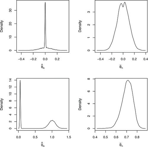For instance, consider the situation where n = 100, p = 2, X₁ ∼ N(0, 1), X₂ = 20X₁ + η, where η ∼ N(0, 1) is independent of X₁, and (1) $$\begin{array}{c}\hfill Y=X_1+ϵ,\end{array}$$(1) where ε ∼ N(0, 1) is independent of X₁ (and η). Instead of using adaptive resampling test (ART) to obtain the critical value for the test of size α = 0.05, we simply simulated from the null model where (X₁, X₂) are as above, but Y = ε ∼ N(0, 1). A density plot of the values of ${\widehat{\theta }}_n$ computed over 10,000 repetitions is shown in the top-left panel of Figure 1; note that the spike around 0 is due mainly to the 5017 occasions where X₂ happened to have higher absolute correlation with Y (i.e., ${\widehat{k}}_n=2$). The critical value for the test was taken to be the 100(1 − α)th quantile of the realizations of $|{\widehat{\theta }}_n|$, namely, 0.171. Under the alternative specified by (2.1(1) $$\begin{array}{c}\hfill Y=X_1+ϵ,\end{array}$$(1) ), ${\widehat{\theta }}_n$ has a highly bimodal distribution as illustrated in the bottom-left panel of Figure 1. The only occasions when we were able to reject the null were when X₁ had higher absolute correlation with Y, yielding a power of 59.8%.

Fortunately, it is straightforward to construct a slightly modified test statistic that can yield great improvements. Indeed, it is standard practice in variable selection contexts to standardize each predictor X_k so that $\widehat{\mathrm{E}}\left(X_k\right)=0$ and $\widehat{\text{v}\mathrm{ar}}\left(X_k\right)=n$, and likewise to standardize the response so that $\widehat{\mathrm{E}}\left(Y\right)=0$ and $\widehat{\text{v}\mathrm{ar}}\left(Y\right)=n$. This amounts to using the test statistic $|{\tilde{\theta }}_n|$, where $$\begin{array}{c}\hfill {\tilde{\theta }}_n=\widehat{\mathrm{Corr}}(X_{{\widehat{k}}_n},Y).\end{array}$$Note that the definition of ${\tilde{\theta }}_n$ does not depend on whether the predictors and the response have been standardized or not, and that we have the simple expression $$\begin{array}{c}\hfill |{\tilde{\theta }}_n|=\underset{j=1,...,p}{max}\left|\widehat{\mathrm{Corr}}(X_j,Y)\right|.\end{array}$$For the example above, the top-right panel of Figure 1 gives a density plot of ${\tilde{\theta }}_n$ under the null; the critical value for our modified test was 0.198. Under the alternative, ${\tilde{\theta }}_n$ tends to be inflated, regardless of whether ${\widehat{k}}_n=1$ or ${\widehat{k}}_n=2$; in fact, we obtain an empirical power of 100%.

Figure 1 Top row: density plots of ${\widehat{\theta }}_n$ (left) and ${\tilde{\theta }}_n$ (right) under the global null hypothesis for the example in Section 2. Bottom row: corresponding density plots of ${\widehat{\theta }}_n$ (left) and ${\tilde{\theta }}_n$ (right) under the alternative specified in (2.1(1) $$\begin{array}{c}\hfill Y=X_1+ϵ,\end{array}$$(1) ).

We emphasize that the problems described in this section are not observed in the simulation study of the article because there all of the predictors have equal variance. In the next section, we consider predictors and response standardized as above, and consider alternative approaches to calibrate the test statistic $n^{1/2}\left|{\tilde{\theta }}_n\right|$, as well as another test statistic proposed in Goeman, van de Geer, and van Houwelingen (2006).

3. ALTERNATIVE APPROACHES

Although the nonregularities in the problem considered here make the construction of a confidence interval for θ₀ a challenging task, the particularly simple form of the global null hypothesis makes the testing problem amenable to several other approaches. Under the global null, X and Y are independent, so by the central limit theorem, $$\begin{array}{c}\hfill n^{1/2}\left(\begin{array}{c}\widehat{\mathrm{Corr}}(X_1,Y)\hfill \\ ⋮\hfill \\ \widehat{\mathrm{Corr}}(X_p,Y)\hfill \end{array}\right)\stackrel{d}{\to }{N}_p(0,\Theta ),\end{array}$$as n → ∞, where Θ_jk = Corr(X_j, X_k). Then by the continuous mapping theorem, $$\begin{array}{c}\hfill n^{1/2}|{\tilde{\theta }}_n|\stackrel{d}{\to }\underset{j=1,...,p}{max}\left|Z_j\right|,\end{array}$$where (Z₁, …, Z_p)^T ∼ N_p(0, Θ). 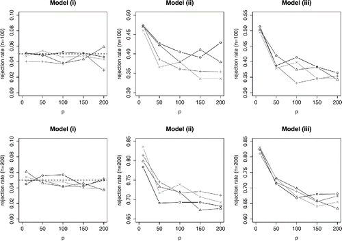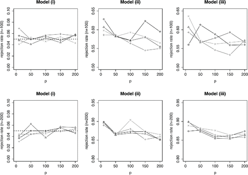Since the distribution on the right does not depend on the distribution of Y, we can simulate $n^{1/2}\left|{\tilde{\theta }}_n\right|$ under the distribution of Y being (a) the empirical measure of the data Y₁, …, Y_n, or (b) N(0, 1), for example, to calibrate the test statistic. Figures 2 and 3 display the results of using these approaches in the numerical experiments of Section 4.1 in the article. Method (a) appears to yield a test with size not exceeding its nominal level and with similar power to the ART procedure. When the error distribution is normal, the size of the test from method (b) is exactly equal to the nominal level, up to Monte Carlo error; again the power in similar to that of ART.

Figure 2 The same graphs as in Figure 1 (ρ = 0.5) of the original article but for globaltest (black circles), method (a) (green crosses), method (b) (red plus signs), and the permutation test (blue triangles). Note model (i) is the null model. (For interpretation of the references to color in this caption and that of Figure 3, the reader is referred to the web version of the article.)

Figure 3 The same graphs as in Figure 2 (ρ = 0.8) of the original article but for globaltest (black circles), method (a) (green crosses), method (b) (red plus signs), and the permutation test (blue triangles).

An alternative approach to calibration is via permutations. Making the dependence of ${\tilde{\theta }}_n$ on Y₁, …, Y_n explicit, we note that the law of ${\tilde{\theta }}_n(Y_1,...,Y_n)$ is the same as that of ${\tilde{\theta }}_n(Y_{\pi \left(1\right)},...,Y_{\pi \left(n\right)})$ for any permutation π of {1, …, n}. The permutation test has the advantage over (a) and (b), of having its size not exceeding the nominal level regardless of the distribution of Y. Its power performance also seems close to that of ART.

Although it may seem natural to base test statistics on ${\tilde{\theta }}_n$, there are other possibilities. For example, Goeman, van de Geer, and van Houwelingen (2006) constructed a locally most powerful test for high-dimensional alternatives under the global null. We compare the power of their globaltest procedure with the approaches discussed above, in Figures 2 and 3. Overall, its performance is similar to that of ART, though in certain settings it seems to have a slight advantage and in others a slight disadvantage.

4. EXTENSIONS

In our view, the main attraction of ART is that it can be used to construct confidence intervals for θ_n. It would be interesting to study empirically the coverage properties and lengths of these intervals. Another interesting related question would be to try to provide some form of uncertainty quantification for the variable having greatest absolute correlation with the response. The ideas of stability selection (Meinshausen and Bühlmann 2010; Shah and Samworth 2013) provide natural quantifications of variable importance through empirical selection probabilities over subsets of the data. However, it is not immediately clear how to use these to provide, say, a (nontrivial) confidence set of variable indices that with at least 1 − α probability contains all indices of variables having largest absolute correlation with the response (in particular this would be set full set {1, …, p} of indices under the global null).

Although understanding marginal relationships between variables and the response is useful in certain contexts, in other situations, the coefficients from multivariate regression are of more interest. It would be interesting to see whether the ART methodology can be extended to provide confidence intervals for the largest regression coefficients in absolute value.

Additional information

Notes on contributors

Rajen D. Shah

Rajen D. Shah (E-mail: [email protected]) and Richard J. Samworth (E-mail: [email protected]), Statistical Laboratory, University of Cambridge, Cambridge CB2 1TN, United Kingdom. The second author is supported by an Engineering and Physical Sciences Research Council Fellowship and a grant from the Leverhulme Trust.

Richard J. Samworth

Rajen D. Shah (E-mail: [email protected]) and Richard J. Samworth (E-mail: [email protected]), Statistical Laboratory, University of Cambridge, Cambridge CB2 1TN, United Kingdom. The second author is supported by an Engineering and Physical Sciences Research Council Fellowship and a grant from the Leverhulme Trust.

REFERENCES

- Beran, R.J. (1997), “Diagnosing Bootstrap Success,” Annals of the Institute of Statistical Mathematics, 4, 1–24.
- Chatterjee, A., and Lahiri, S.N. (2011), “Bootstrapping Lasso Estimators,” Journal of the American Statistical Association, 106, 608–625.
- Fan, J., and Lv, J. (2008), “Sure Independence Screening for Ultrahigh Dimensional Feature Space” (with discussion), Journal of the Royal Statistical Society, Series B, 70, 849–912.
- Fan, J., Samworth, R., and Wu, Y. (2009), “Ultrahigh Dimensional Feature Selection: Beyond the Linear Model,” Journal of Machine Learning Research, 10, 2013–2038.
- Goeman, J.J., van de Geer, S.A., and van Houwelingen, H.C. (2006), “Testing Against a High Dimensional Alternative,” Journal of the Royal Statistical Society, 68, 477–493.
- Laber, E., and Murphy, S.A. (2011), “Adaptive Confidence Intervals for the Test Error in Classification” (with discussion), Journal of the American Statistical Association, 106, 904–913.
- Meinshausen, N., and Bühlmann, P. (2010), “Stability Selection” (with discussion), Journal of the Royal Statistical Society, Series B, 72, 417–473.
- Samworth, R. (2003), “A Note on Methods of Restoring Consistency to the Bootstrap,” Biometrika, 90, 985–990.
- ——— (2005), “Small Confidence Sets for the Mean of a Spherically Symmetric Distribution,” Journal of the Royal Statistical Society, Series B, 67, 343–361.
- Shah, R.D., and Samworth, R.J. (2013), “Variable Selection With Error Control: Another Look at Stability Selection,” Journal of the Royal Statistical Society, Series B, 75, 55–80.