On the Reproducibility of Psychological Science

ABSTRACT

Investigators from a large consortium of scientists recently performed a multi-year study in which they replicated 100 psychology experiments. Although statistically significant results were reported in 97% of the original studies, statistical significance was achieved in only 36% of the replicated studies. This article presents a reanalysis of these data based on a formal statistical model that accounts for publication bias by treating outcomes from unpublished studies as missing data, while simultaneously estimating the distribution of effect sizes for those studies that tested nonnull effects. The resulting model suggests that more than 90% of tests performed in eligible psychology experiments tested negligible effects, and that publication biases based on p-values caused the observed rates of nonreproducibility. The results of this reanalysis provide a compelling argument for both increasing the threshold required for declaring scientific discoveries and for adopting statistical summaries of evidence that account for the high proportion of tested hypotheses that are false. Supplementary materials for this article are available online.

Keywords:

• Bayes factor
• Null hypothesis significance test
• Posterior model probability
• Publication bias
• Reproducibility
• Significance test

1. Introduction

Reproducibility of experimental research is essential to the progress of science, but there is growing concern over the failure of scientific studies to replicate (e.g., Ioannidis 2005; Prinz et al. 2011; Begley and Ellis 2012; Pashler and Wagenmakers 2012; McNutt 2014). This concern has become particularly acute in the social sciences, where the effects of publication bias and other sources of nonreproducibility are now widely recognized, and a number of researchers have gone as far as to propose new methods for detecting irregularities in reported test results (Francis 2013; Simonsohn et al. 2014). Motivated by this concern, the Open Science Collaboration (OSC) recently undertook a multi-year study that replicated 100 scientific studies selected from three prominent psychology journals: Psychological Science, Journal of Personality and Social Psychology, and Journal of Experimental Psychology: Learning, Memory, and Cognition (OSC 2015). The goal of their project was to assess the reproducibility of studies in psychology and to potentially identify factors that were associated with low reproducibility rates. The OSC concluded that “replication effects were half the magnitude of original effects” and that while 97% of the original studies had statistically significant results, only 36% of replications did.

To conduct their study, the OSC developed a comprehensive protocol for selecting the psychology experiments that were subsequently replicated. This protocol specified “the process of selecting the study and key effect from the available articles, contacting the original authors for study materials, preparing a study protocol and analysis plan, obtaining review of the protocol by the original authors and other members within the present project, registering the protocol publicly, conducting the replication, writing the final report, and auditing the process and analysis for quality control” (OSC 2015, aac4716-1). Full details regarding the selection of articles from which experiments were selected for replication, along with the procedures used to replicate and report results from these experiments, can be found in the original OSC article.

The essential feature of the OSC study is that it provides an approximately representative sample of psychology experiments that led to successful publication in one of three leading psychology journals in which the same effects were measured twice in independent replications. As we demonstrate below, these replications make it possible to estimate the effect size of each study even after accounting for publication bias. We exploit this feature of the OSC study to describe a statistical model that provides a quantitative explanation for the low reproducibility rates observed in the OSC article. We also estimate several quantities needed to compute the posterior probabilities of hypotheses tested in those and future studies. In particular, we use the OSC data to estimate the distribution of effect sizes across psychology studies, as well as the proportion of hypotheses tested in psychology that are true.

Our analyses suggest that the proportion of experimental hypotheses tested in psychology that are false likely exceeds 90%. In other words, if one implicitly accounts for the number of statistical analyses that are conducted, the number of statistical tests that are performed, the choice of which test statistics are actually calculated and the filtering out of nonsignificant p-values in the publication process, then the observed replication rates in psychology can be well explained by assuming that 90% or more of statistical hypothesis tests test null hypotheses that are true. When evaluating a published p-value that is 0.05, this means that the probability that the tested null hypothesis was actually true likely exceeds 0.90 (based on the distribution of effect sizes estimated from the OSC data). That is, the false positive rate for p = 0.05 discoveries is also over 90%. This fact has important ramifications for the interpretation of p-values derived from experiments conducted in psychology, and likely in many other fields as well.

2. Subset Selection and Publication Bias

While the authors of OSC (2015) replicated 100 psychology experiments, many of their findings were based on a subset of these experiments in which it was possible to transform observed effect sizes to the correlation scale. Their rationale for analyzing correlation coefficients was based on the easy interpretation of correlation coefficients and the fact that, after application of Fisher's z-transformation (Fisher 1915), the approximate standard errors of the transformed coefficients were a function only of the study sample size. The subset of OSC data for which Fisher's transformation provided both a transformed correlation coefficient and a standard error for this coefficient was labeled the Meta-Analytic (MA) subset. The MA subset included studies that based their primary findings on the report of t statistics, F statistics with one degree of freedom in the numerator, and correlation coefficients. There were 73 studies in the MA subset. The data and code for the OSC study are available at https://osf.io/ezcuj (z-transformed correlation coefficients are stored in R variables $\mathtt{final}\$\mathtt{fis}.\mathtt{o}$ and $\mathtt{final}\$\mathtt{fis}.\mathtt{r}$, which are created by the source file $\mathtt{masterscript}.\mathtt{R}$).

Recall that for a sample correlation coefficient r based on a bivariate normal sample of size n having population correlation coefficient ρ, the sampling distribution of (1) $$z=\frac{1}{2}ln\left(\frac{1+r}{1-r}\right)$$(1) is approximately normally distributed with mean (2) $$\zeta =\frac{1}{2}ln\left(\frac{1+\rho }{1-\rho }\right)$$(2) and variance 1/(n − 3) (Fisher 1915).

As in the OSC study, analyzing z-transformed correlation coefficients also simplifies our model for effect sizes across studies. For this reason, we too restrict attention to the MA subset of studies in the analyses that follow. Although this decision results in some loss of efficiency, our decision to restrict attention to the MA subset of studies, which is based solely on the type of test statistic used to summarize results in the original studies, does not introduce any obvious biases in the estimation of our primary quantity of interest, the proportion of tested psychology hypotheses that are true. It also facilitates our examination of the statistical properties of the distribution of nonnull effect sizes on a common scale.

Publication bias (the tendency to select test statistics that are statistically significant and to then publish only positive findings) is now generally regarded as a primary cause of nonreproducibility of scientific findings. We note that publication bias played a prominent role in the American Statistical Association's recent statement on statistical significance and p-values (Wasserstein and Lazar 2016), and alarm over its effects on the reproducibility of science is increasing (e.g., Fanelli 2010; Franco et al. 2014; Peplow 2014). Hence, another important decision that affects the formulation of our statistical model involves the manner in which we model publication bias. As noted previously, 97% of the studies included in the OSC experiment originally reported statistically significant findings. This pattern is also exhibited in the MA subset of studies, in which 70 out of 73 (96%) studies reported statistically significant findings. (We note that among the original 100 studies, four p-values between 0.050 and 0.052 were deemed significant; three of these “significant” p-values are included in the MA subset.)

The high proportion of studies that reported statistically significant findings suggests a severe publication bias in the hypothesis tests that were reported. We adopt a missing data framework (e.g., Tanner and Wong 1987; Little and Rubin 2014) to account for this bias, and explicitly assume the existence of an unobserved population of hypothesis tests and test statistics that were calculated in the OSC sampling frame. This population of hypothesis tests includes tests that resulted in (a) test statistics derived from experiments that obtained statistically significant findings and were published, (b) test statistics that would have been published had they obtained statistical significance but did not, and (c) test statistics that were published even though they did not obtain statistically significant findings. In stating these assumptions we have intentionally emphasized the distinction between an experimental outcome and the report of a test statistic. We have made this distinction to emphasize the fact that researchers often have the choice of reporting numerous test statistics based on the same experiment, and that in practice they often choose to report only test statistics that yield significant p-values (Simmons et al. 2011).

Because we have restricted our attention to the MA subset of studies, we also restrict our hypothetical population of hypothesis tests to tests that based their primary outcome on a t, F_{1, ν}, or correlation statistic. The unknown size of this population is denoted by M. A primary goal of our analysis is to estimate the proportion of studies in this population that tested true null hypotheses, as well as the distribution of effect sizes among studies for which the null hypothesis was false.

3. A Statistical Model for the OSC Data

The assumptions and notation underlying our statistical model for the OSC replication data can now be stated more precisely as follows^{Figure 1}:

1.	The 73 z-transformed correlation coefficients reported in the MA subset of studies represent a sample from a larger population of M hypothesis tests that would have been published had they either obtained a statistically significant result or had been unique in some other way.
2.	Within this population of M hypothesis tests, a test that produced a statistically “significant” finding was always published. To account for the fact that three studies were deemed significant for p-values that were slightly above 0.05, in the analyses that follow we define a “significant” p-value to be a value less than 0.052. The conclusions of our analyses are unaffected by this assumption and it simplifies exposition of our statistical model.
3.	Tests that resulted in an insignificant p-value were published with probability α. Conversely, tests that produced an insignificant p-value were not published with probability (1 − α).
4.	Test statistics obtained from different tests are statistically independent. Of course, this assumption is only an approximation to reality and is unlikely to apply to the multitude of tests that a researcher might calculate from the same set of data. To the extent that there is dependence within this population of test statistics, we adjust our interpretation of M as being the “effective sample size” or effective number of independent tests that were conducted.
5.	The distribution of transformed effect sizes among those experiments that tested a false null hypothesis (i.e., that had nonzero effect sizes) is described by either (i) a (normal) moment density function indexed by a parameter τ (Johnson and Rossell 2010), or (ii) a mean zero normal density function with variance τ. The moment density function can be expressed as (3) $$f\left(\zeta |\tau \right)=\frac{{\zeta }^2}{\sqrt{2\pi {\tau }^3}}exp\left(-\frac{{\zeta }^2}{2\tau }\right),$$(3) where ζ denotes the transformed population correlation coefficient from (2(2) $$\zeta =\frac{1}{2}ln\left(\frac{1+\rho }{1-\rho }\right)$$(2) ). The normal prior density function for the transformed effect sizes is parameterized as (4) $$f\left(\zeta |\tau \right)=\frac{1}{\sqrt{2\pi \tau }}exp\left(-\frac{{\zeta }^2}{2\tau }\right).$$(4)
6.	We adopt the common convention used by the original authors of the MA studies and approximate “small interval” hypotheses (e.g., (− ε, ε), ε ≪ 1) by point null hypotheses. A discussion of the implications and adequacy of this approximation for various values of ε are discussed in, for example, Berger and Delampady (1987, sec. 2). For a specified test statistic T(X), they note that the adequacy of the small interval approximation to a point null hypothesis depends only on the adequacy of $$P_{{\theta }_0}\left(\right|T\left(X\right)|\ge \left|t\right|)$$in approximating $$\underset{\theta :|\theta -{\theta }_0|\le ϵ}{sup}{P}_{\theta }\left(\right|T\left(X\right)|\ge \left|t\right|).$$We assume this approximation is adequate for the studies included the MA subset.

The proportion of the M studies that tested true null hypotheses (i.e., had effect sizes that were negligible) is denoted by π₀.

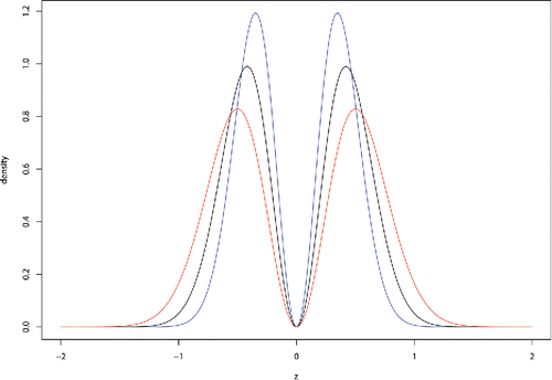
In the fifth assumption, two models have been specified for the prior distribution on the effect sizes under the alternative hypotheses. The moment density explicitly parameterizes the assumption that effect sizes under alternative hypotheses cannot be equal or be too close to 0. The use of the moment prior density may thus alleviate concerns regarding the approximation of small interval null hypotheses by point null hypotheses. This feature of the moment prior is illustrated in Figure 1, where it is seen that the moment prior density is identically equal to 0 when ζ = 0. The moment prior is a special case of a nonlocal alternative prior density.

Figure 1. Normal moment prior. This density function is used to model the marginal distribution of z-transformed effect sizes when the alternative hypothesis is true. The curves in blue, black, and red represent the moment priors corresponding to τ = 0.060, 0.088, and 0.125, respectively. These values correspond to the lower (blue) and upper (red) boundaries of the 95% credible interval and posterior mean (black) for τ based on the OSC data.

The normal prior density described in assumption 5 is proposed as a contrast to the moment prior. The shape of this density embodies the belief that the nonnull effect sizes are likely to concentrate near 0 even when the alternative hypothesis is true. The normal prior is an example of a local alternative prior density.

In Section 5, we compare the adequacy of these two models in fitting the transformed correlation coefficients obtained from the MA subset of studies. Using a Bayesian chi-squared statistic to assess model fit (Johnson 2004), we find that the moment prior density provides an adequate model for the transformed population coefficients, whereas the normal prior does not. Nonetheless, parameter estimates obtained under the normal model provide an indication of the sensitivity of our conclusions to prior assumptions regarding the distribution of nonnull effect sizes, and so we describe methodology and results for both models below.

For a given value of M, we let z^M = {z^M_ij} denote the transformed sample correlation coefficient (1(1) $$z=\frac{1}{2}ln\left(\frac{1+r}{1-r}\right)$$(1) ) for test i (i = 1, …, M), replication j (1 = original test, 2 = replicated test), and let n^M = {n^M_ij} denote the corresponding sample sizes. The vector ${\mathbf{\zeta }}^M=\left\{{\zeta }_i^M\right\}$ denotes the z-transformed population correlations for each test i, and R^M = {R^M_i} denotes a vector of indicators of whether the original test statistic i was published (1 if yes, 0 if no). For i = 1, …, 73, it follows that R^M_i = 1; for i = 74, …, M it follows that R^M_i = 0. Similarly, we let S^M = {S^M_i} denote a vector of indicators of whether the original studies resulted in statistically significant results (i.e., p < 0.052). By assumption, P(R^M_i = 1|S_i^M = 0) = α, and P(R^M₁ = 1|S_i^M = 1) = 1.

To simplify notation, we suppress the dependence of z, $\mathbf{\zeta }$, R, S, and n on M in what follows. We also let φ(x | μ, σ²) denote the value of a Gaussian (normal) density function with mean μ and variance σ² evaluated at x, and denote the variance of z_ij by σ²_ij = 1/(n_ij − 3). The generic symbols for a density function and conditional density function are f( · ) and f( ·  |  · ), respectively.

Given this notation, the (marginal) sampling density for a z-transformed correlation in study (i, j) is φ[z_ij | ζ_i, σ²_ij]. The joint sampling density for various values of z_ij, R_i, and S_i can be specified as follows:

1.	For Ri = 1, Si = 1, j = 1, $$f(z_{i1},R_i=1,S_i=1|{\zeta }_i)=\varphi [z_{i1}|{\zeta }_i,{\sigma }_{ij}^2]\mathrm{Ind}\left(\right|z_{i1}|>b_i),$$where bi = qγ σij and qγ is the γ = 0.974 quantile from a standard normal density (γ = 0.974 is used instead of γ = 0.975 to account for the fact that p-values of 0.052 were considered to be significant in the OSC data).
2.	For Ri = 1, Si = 0, j = 1, $$f(z_{i1},R_i=1,S_i=0|{\zeta }_i)=\alpha \varphi [z_{i1}|{\zeta }_i,{\sigma }_{ij}^2]Ind\left(\right|z_{i1}|\le b_i).$$
3.	For Ri = 0, Si = 0, j = 1, $$\begin{array}{ccc}& & f(z_{i1},R_i=0,S_i=0|{\zeta }_i)\hfill \\ & & =(1-\alpha )\varphi [z_{i1}|{\zeta }_i,{\sigma }_{ij}^2]Ind\left(\right|z_{i1}|\le b_i),\hfill \end{array}$$where the value of zi1 is regarded as missing data for i > 73 (Tanner and Wong 1987; Little and Rubin 2014).
4.	For replicated studies (j = 2), the sampling density of a transformed correlation is simply $$f\left(z_{i2}\right|{\zeta }_i)=\varphi \left[z_{i2}|{\zeta }_i,{\sigma }_{ij}^2\right],$$independently of (Ri, Si). For i > 73, the value of zi2 is regarded as missing data.

To specify the prior density on the effect sizes, we introduce a vector of variables W = {W_i} (again suppressing dependence on M) whose components equal 0 if ζ_i = 0 (i.e., the null hypothesis of no effect pertains) and equal 1 if ζ_i is drawn from either a moment distribution or a normal distribution. A priori, we assume W_i is Bernoulli with success probability 1 − π₀, reflecting the fact that the marginal probability of the null hypothesis is π₀. Under the moment prior model, the prior density on ζ_i, i = 1, …, M, given W_i and τ can be expressed as (5) $$f\left({\zeta }_i\right|\tau ,W_i)=(1-W_i){\delta }_0+W_i\frac{{\zeta }_i^2}{{\tau }^{3/2}\sqrt{2\pi }}exp\left(-\frac{{\zeta }_i^2}{2\tau }\right),$$(5) where δ₀ denotes a unit mass at 0. Similarly, under the normal prior model, the prior density on ζ_i, i = 1, …, M, given W_i and τ can be expressed as (6) $$f\left({\zeta }_i\right|\tau ,W_i)=(1-W_i){\delta }_0+W_i\frac{1}{\sqrt{2\pi \tau }}exp\left(-\frac{{\zeta }_i^2}{2\tau }\right).$$(6)

A parametric model is not specified for the unobserved sample size vectors for unpublished studies. Instead, pairs of values of (n_i1, n_i2) were sampled with replacement from the empirically observed distribution of sample sizes from the meta-analysis (MA) subset within a given Markov chain Monte Carlo (MCMC) run, and results from several runs of the MCMC algorithm were combined to obtain samples from the joint distribution on all parameters of interest. A Jeffreys’ prior for a Bernoulli success probability was assumed for α and π₀, and a prior proportional to 1/τ was assumed for τ (this is the noninformative prior for τ under both the moment and normal prior model). Finally, we assume that the prior on M is proportional to M^{− 2} for M = 1, 2, ….

Given these model assumptions, it follows that the joint posterior distribution can be expressed as (7) $$f(\mathbf{z},\mathbf{\zeta },\mathbf{W},M,{\pi }_0,\tau ,\alpha |D)\propto \left(\genfrac{}{}{0pt}{}{M}{703}\right)\prod _{\begin{array}{c}{R}_i=1\\ S_i=1\\ j=1,2\end{array}}f(z_{ij},R_i,S_i|{\zeta }_i)$$(7) (8) $$\times \prod _{\begin{array}{c}{R}_i=1\\ S_i=0\\ j=1,2\end{array}}f(z_{ij},R_i,S_i|{\zeta }_i)$$(8) (9) $$\times \prod _{\begin{array}{c}{R}_i=0\\ S_i=0\\ j=1,2\end{array}}f(z_{ij},R_i,S_i|{\zeta }_i)$$(9) (10) $$\times \prod _{i=1}^{M}f\left({\zeta }_i\right|\tau ,W_i){\pi }_0^{1-W_i}{(1-{\pi }_0)}^{W_i}$$(10) (11) $$\times \frac{1}{\tau M^2}{\left({\pi }_0\alpha \right)}^{-\frac{1}{2}}{(1-{\pi }_0)}^{-\frac{1}{2}}{(1-\alpha )}^{-\frac{1}{2}},$$(11) where D represents {z_ij}, R_i = 1, and S_i for i = 1, …, 73. For i > 73, it follows from model assumptions that R_i = S_i = 0. The combinatorial term at the beginning of the right-hand product is necessary to account for the number of ways that the 70 published studies with significant test statistics, three published studies with insignificant test statistics, and M − 73 unpublished studies with insignificant test statistics could have occurred among the collection of M studies performed. The density in line (10(10) $$\times \prod _{i=1}^{M}f\left({\zeta }_i\right|\tau ,W_i){\pi }_0^{1-W_i}{(1-{\pi }_0)}^{W_i}$$(10) ) refers to either the moment density from (5(5) $$f\left({\zeta }_i\right|\tau ,W_i)=(1-W_i){\delta }_0+W_i\frac{{\zeta }_i^2}{{\tau }^{3/2}\sqrt{2\pi }}exp\left(-\frac{{\zeta }_i^2}{2\tau }\right),$$(5) ) or the normal density from (6(6) $$f\left({\zeta }_i\right|\tau ,W_i)=(1-W_i){\delta }_0+W_i\frac{1}{\sqrt{2\pi \tau }}exp\left(-\frac{{\zeta }_i^2}{2\tau }\right).$$(6) ), depending on the model that is being applied.

The joint posterior density function described in (7(7) $$f(\mathbf{z},\mathbf{\zeta },\mathbf{W},M,{\pi }_0,\tau ,\alpha |D)\propto \left(\genfrac{}{}{0pt}{}{M}{703}\right)\prod _{\begin{array}{c}{R}_i=1\\ S_i=1\\ j=1,2\end{array}}f(z_{ij},R_i,S_i|{\zeta }_i)$$(7) )–(11(11) $$\times \frac{1}{\tau M^2}{\left({\pi }_0\alpha \right)}^{-\frac{1}{2}}{(1-{\pi }_0)}^{-\frac{1}{2}}{(1-\alpha )}^{-\frac{1}{2}},$$(11) ) describes a density function on a high-dimensional parameter space in which the dimensions of several model parameters vary with M. However, our primary interest lies in performing inference on the parameters (M, π₀, α, τ). To simplify this task, we now describe the marginal distribution on the parameters of interest, obtained by marginalizing over the nuisance parameters z, $\mathbf{\zeta }$, and $\mathbf{W}$. The following lemmas are useful in describing this marginal posterior density function.

Lemma 1.

Assume that the nonnull effect sizes are drawn from the moment prior density given in (5(5) $$f\left({\zeta }_i\right|\tau ,W_i)=(1-W_i){\delta }_0+W_i\frac{{\zeta }_i^2}{{\tau }^{3/2}\sqrt{2\pi }}exp\left(-\frac{{\zeta }_i^2}{2\tau }\right),$$(5) ). For a given value of M and i ⩽ 73, define $$\begin{array}{ccc}\hfill A_i(\alpha ,{\pi }_0,\tau )& =& \int f\left({\zeta }_i\right|\tau ,W_i){\pi }_0^{1-W_i}{(1-{\pi }_0)}^{W_i}\hfill \\ & \times & \prod _{j=1}^{2}f(z_{ij},R_i,S_i|{\zeta }_i)d{\zeta }_{i}d{W}_i,\hfill \end{array}$$and let $$\begin{array}{ccc}\hfill a& =& \frac{1}{2\pi {\sigma }_{i1}{\sigma }_{i2}{\tau }^{3/2}},w=\frac{1}{{\sigma }_{i1}^2}+\frac{1}{{\sigma }_{i2}^2}+\frac{1}{\tau }\hfill \\ \hfill b& =& aexp\left\{-0.5\left[\frac{z_{i1}^2}{{\sigma }_{i1}^2}+\frac{z_{i1}^2}{{\sigma }_{i1}^2}-\frac{1}{w}{\left(\frac{z_{i1}}{{\sigma }_{i1}^2}+\frac{z_{i2}}{{\sigma }_{i2}^2}\right)}^2\right]\right\}.\hfill \end{array}$$Then (12) $$\begin{array}{ccc}& & A_i(\alpha ,{\pi }_0,\tau )={\pi }_0{\alpha }^{1-S_i}\prod _{j=1}^2\varphi \left(z_{ij}|0,{\sigma }_{ij}^2\right)\hfill \\ & & +(1-{\pi }_0){\alpha }^{1-S_i}b{w}^{-3/2}\left[1+\frac{1}{w}{\left(\frac{z_{i1}}{{\sigma }_{i1}^2}+\frac{z_{i2}}{{\sigma }_{i2}^2}\right)}^2\right].\hfill \end{array}$$(12)

Lemma 2.

Assume that the nonnull effect sizes are drawn from the moment prior density given in (5(5) $$f\left({\zeta }_i\right|\tau ,W_i)=(1-W_i){\delta }_0+W_i\frac{{\zeta }_i^2}{{\tau }^{3/2}\sqrt{2\pi }}exp\left(-\frac{{\zeta }_i^2}{2\tau }\right),$$(5) ), suppose tests are conducted at the 2 − 2γ level of significance, and that q_γ is the γ quantile from a standard normal density function. Let Φ( · ) denote the standard normal distribution function. For a given value of M and i > 73, define $$\begin{array}{ccc}\hfill B_i(\alpha ,{\pi }_0,\tau )& =& \int f\left({\zeta }_i\right|\tau ,W_i){\pi }_0^{1-W_i}{(1-{\pi }_0)}^{W_i}\hfill \\ & \times & \prod _{j=1}^{2}f(z_{ij},R_i,S_i|{\zeta }_i)d{z}_{i1}d{z}_{i2}d{\zeta }_{i}d{W}_i,\hfill \end{array}$$and let $$\begin{array}{ccc}\hfill c& =& \frac{1}{{\sigma }_{i1}^2}+\frac{1}{\tau },d=\frac{1}{{\sigma }_{i1}^2}-\frac{1}{c{\sigma }_{i1}^4},\hfill \\ \hfill f& =& \sqrt{d}{q}_{\gamma },g=\Phi \left(f\right)-\Phi (-f),\hfill \end{array}$$and $$h=\frac{1}{{\sigma }_{i1}\sqrt{{\tau }^{3}d{c}^3}}\left\{\frac{1}{cd{\sigma }_{i1}^4}\left[g-\sqrt{\frac{2}{\pi }}fexp\left(-\frac{f^2}{2}\right)\right]+g\right\}.$$Then (13) $$B_i(\alpha ,{\pi }_0,\tau )=(1-\alpha )\left[(1-{\pi }_0)h+{\pi }_0(2\gamma -1)\right].$$(13)

Lemma 3.

Assume that the nonnull effect sizes are drawn from the normal prior density given in (6(6) $$f\left({\zeta }_i\right|\tau ,W_i)=(1-W_i){\delta }_0+W_i\frac{1}{\sqrt{2\pi \tau }}exp\left(-\frac{{\zeta }_i^2}{2\tau }\right).$$(6) ). For a given value of M and i ⩽ 73, define A_i(α, π₀, τ) according to $$\begin{array}{ccc}\hfill A_i(\alpha ,{\pi }_0,\tau )& =& \int f\left({\zeta }_i\right|\tau ,W_i){\pi }_0^{1-W_i}{(1-{\pi }_0)}^{W_i}\hfill \\ & \times & \prod _{j=1}^{2}f(z_{ij},R_i,S_i|{\zeta }_i)d{\zeta }_{i}d{W}_i,\hfill \end{array}$$and let $$\begin{array}{c}\hfill a^{*}=\frac{1}{2\pi {\sigma }_{i1}{\sigma }_{i2}{\tau }^{1/2}},w^{*}=\frac{1}{{\sigma }_{i1}^2}+\frac{1}{{\sigma }_{i2}^2}+\frac{1}{\tau },\end{array}$$and $$\begin{array}{c}\hfill b^{*}=a^{*}exp\left\{-0.5\left[\frac{z_{i1}^2}{{\sigma }_{i1}^2}+\frac{z_{i2}^2}{{\sigma }_{i2}^2}-\frac{1}{w^{*}}{\left(\frac{z_{i1}}{{\sigma }_{i1}^2}+\frac{z_{i2}}{{\sigma }_{i2}^2}\right)}^2\right]\right\}.\end{array}$$Then $$\begin{array}{ccc}\hfill A_i(\alpha ,{\pi }_0,\tau )& =& {\pi }_0{\alpha }^{1-S_i}\prod _{j=1}^2\varphi \left[z_{ij}\right|0,{\sigma }_{ij}^2]\hfill \\ & & +(1-{\pi }_0){\alpha }^{1-S_i}{b}^{*}{w^{*}}^{-1/2}.\hfill \end{array}$$

Lemma 4.

Assume that the nonnull effect sizes are drawn from the normal prior density given in (6(6) $$f\left({\zeta }_i\right|\tau ,W_i)=(1-W_i){\delta }_0+W_i\frac{1}{\sqrt{2\pi \tau }}exp\left(-\frac{{\zeta }_i^2}{2\tau }\right).$$(6) ). For a given value of M and i ⩾ 73, define B_i(α, π₀, τ) according to $$\begin{array}{ccc}\hfill B_i(\alpha ,{\pi }_0,\tau )& =& \int f\left({\zeta }_i\right|\tau ,W_i){\pi }_0^{1-W_i}{(1-{\pi }_0)}^{W_i}\hfill \\ & \times & \prod _{j=1}^{2}f(z_{ij},R_i,S_i|{\zeta }_i)d{z}_{i1}d{z}_{i2}d{\zeta }_{i}d{W}_i.\hfill \end{array}$$Let $$\begin{array}{ccc}\hfill c^{*}& =& \frac{1}{{\sigma }_{i1}^2}+\frac{1}{\tau },d^{*}=\frac{1}{{\sigma }_{i1}^2}-\frac{1}{c^{*}{\sigma }_{i1}^4},\hfill \\ \hfill f^{*}& =& \sqrt{d^{*}}{b}_i=\sqrt{d^{*}}{q}_{\gamma }{\sigma }_{i1},g^{*}=\Phi \left(f^{*}\right)-\Phi (-f^{*}),\hfill \end{array}$$and $$\begin{array}{c}\hfill h^{*}=\frac{g^{*}}{\sqrt{\tau c^{*}{d}^{*}}{\sigma }_{i1}}.\end{array}$$Then $$\begin{array}{c}\hfill B_i(\alpha ,{\pi }_0,\tau )=(1-\alpha )[(1-{\pi }_0)h^{*}+{\pi }_0(2\gamma -1)].\end{array}$$

Proofs of the Lemmas 1 and 2 appear in the Supplementary Material; the proofs of Lemmas 3 and 4 are similar to their moment analogs.

Based on these lemmas, it follows that the marginal posterior distribution on (M, α, π₀, τ) can be expressed as (14) $$\begin{array}{ccc}& & f(M,\alpha ,{\pi }_0,\tau |D)\hfill \\ & & \propto \left(\genfrac{}{}{0pt}{}{M}{703}\right)\prod _{i=1}^{73}{A}_i(\alpha ,{\pi }_0,\tau )\prod _{i=74}^M{B}_i(\alpha ,{\pi }_0,\tau )\hfill \\ & & \times \frac{1}{\tau M^2}{\left({\pi }_0\alpha \right)}^{-\frac{1}{2}}{(1-{\pi }_0)}^{-\frac{1}{2}}{(1-\alpha )}^{-\frac{1}{2}},\hfill \end{array}$$(14) where the values of A_i and B_i are defined in Lemmas 1 and 2 for the moment prior models, and Lemmas 3 and 4 for the normal prior model on nonnull effect sizes^{Table 1Figure 2}.

The form of the marginal posterior distribution on (M, α, π₀, τ) does not permit explicit calculation of the marginal posterior densities on individual parameters. However, implementing a Markov chain Monte Carlo algorithm to probe this four-dimensional posterior distribution is straightforward.

4. Parameter Estimation

Posterior means and 95% credible intervals for the parameters of interest (M, α, π₀, τ) are provided in Table 1. From this table, we see that the posterior mean of π₀ was approximately 93% under the moment model, while the posterior mean of M was 706. The posterior mean of τ was 0.088. For the normal prior model, the posterior mean of π₀ was slightly smaller—about—89%, as was the posterior mean of M. Qualitatively, the parameter estimates obtained from the two models are very similar. Nonetheless, it is important to examine the extent to which these models fit the distribution of nonnull effect sizes before using them to make inferences about the more general population studies conducted in the field of experimental psychology.

Table 1. Posterior means and 95% credible intervals for model parameters under the moment and normal models for the nonnull effect sizes. Note that the interpretation of τ is not the same in the moment and normal models, whereas the remaining parameter values do have the same interpretation in each model. All results are based on 10 independent runs of an MCMC algorithm. Each run consisted of 10⁵ burn-in iterations, followed by 10⁶ parameter updates.

Model	Parameter	π0	τ	α	M
Moment	Posterior mean	0.930	0.0877	0.00569	706
	Credible interval	(0.884, 0.961)	(0.0604, 0.1252)	(0.00129, 0.0138)	(495, 956)
Normal	Posterior mean	0.886	0.1845	0.00608	669
	Credible interval	(0.800, 0.940)	(0.1121, 0.2983)	(0.00137, 0.01494)	(447, 925)

5. Model Assessment and Comparison

Model assessment in Bayesian hierarchical models can be performed conveniently using pivotal quantities. For our purposes, a pivotal quantity $d(\mathbf{y},\mathbf{\theta })$ is a function of the data and model parameters whose distribution does not depend on unknown parameters. For example, if the components of y = (y₁, …, y_n) are normally distributed with mean μ₀ and variance σ²₀, where μ₀ and σ²₀ are the data-generating (i.e., “true”) parameters, then (15) $$d_1\left[\mathbf{y},\left({\mu }_0,{\sigma }_0^2\right)\right]=\sum _{i=1}^n{\left(\frac{y_i-{\mu }_0}{{\sigma }_0}\right)}^2$$(15) is a pivotal quantity since it has a χ²_n distribution. Johnson (2007) demonstrated that the distribution of a pivotal quantity involving the data $\mathbf{y}$ remains unchanged if a sample from the posterior distribution, say $\tilde{\mathbf{\theta }}$, replaces the data-generating value ${\mathbf{\theta }}_0$ in the definition of the pivotal quantity; Yuan and Johnson (2011) extended this result to pivotal quantities that involve only parameter values.

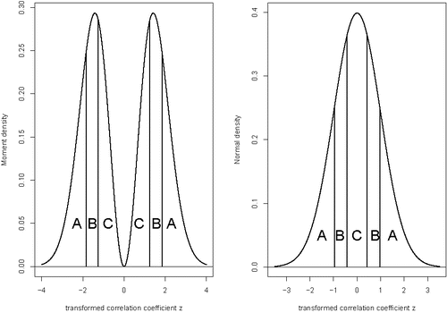
To assess the adequacy^{Figure 3}of the moment and normal prior distributions on the nonnull effect sizes, we use pivotal discrepancy measures based on Pearson's chi-squared goodness-of-fit statistic (Johnson 2004). To this end we partitioned the space of the standardized, transformed population correlations coefficients ζ into three equiprobable, symmetric sets based on the sextiles of the prior distribution on the nonnull effect sizes. This partitioning is illustrated in Figure 2 for both the moment and normal distributions. The choice of cells illustrated in the figure highlights the difference between the moment and normal priors on the transformed correlation coefficients. In particular, cell C encompasses the mode of the normal distribution where the moment prior is 0; the width of this cell is thus much narrower for the normal distribution than it is for the moment distribution. Note that the signs of the transformed sample coefficients were arbitrarily assigned in the OSC data, which motivated the selection of partitioning elements that were symmetric around 0.

Figure 2. Cells used to compute Pearson's chi-squared goodness-of-fit statistic. Left panel: Cells used for moment prior on nonnull effect sizes. Right panel: Cells used for normal prior on nonnull effect sizes. Under both models, the probability assigned to the cells A, B, and C is 1/3.

Next, for each posterior sample of (M, π₀, α, τ) and for each model, we drew a value $\tilde{\mathbf{\zeta }}$ and $\tilde{\mathbf{W}}$ from their full conditional distributions. For observations i judged to be from the alternative hypotheses (i.e., ${\tilde{W}}_i=1$), we assigned ${\tilde{\zeta }}_i/\sqrt{\tau }$ to one of the three cells (A,B,C) depicted in Figure 2. We then constructed Pearson's chi-squared goodness-of-fit statistic based on the $\left|W\right|=\sum {\tilde{W}}_i$ counts assigned to the equiprobable cells. If the assumed model is true, then the resulting statistic is approximately distributed as a chi-squared random variable on 2 degrees of freedom.

The preceding procedure provides a recipe for generating goodness-of-fit statistics that are nominally distributed as χ²₂ random variables. However, statistics based on independent draws of $\tilde{\mathbf{\zeta }}$ and $\tilde{\mathbf{W}}$ from the same posterior distribution are correlated since they are based on the same data. This complicates the calculation of a Bayesian p-value for model adequacy. Instead, it is easier to simply compare the histogram of test statistics produced by repeatedly sampling $\tilde{\mathbf{\zeta }}$ and $\tilde{\mathbf{W}}$ from the posterior distribution, and comparing the resulting pivotal quantities to their nominal distribution. Such a plot is provided in Figure 3. This plot clearly indicates that the Bayesian chi-squared statistics for the moment model are consistent with their nominal χ²₂ distribution, whereas the statistics generated from the normal model are not. This plot provides clear evidence that the normal model is not an appropriate model for the nonnull effect sizes, a result that would likely extend also to other unimodal, local prior densities centered on the null value of 0.

Figure 3. Histogram of posterior samples of Pearson's chi-squared test for goodness of fit under the moment (left panel) and normal prior (right panel) models for the nonnull effect sizes.

Although computing an exact value for a Bayesian p-value for lack-of-fit based on these pivotal quantities would require extensive numerical simulation, we note that bounds on the Bayesian p-value for lack-of-fit can be obtained for the normal model using results in Caraux and Gascuel (1992); Johnson (2007). For the normal model, this p-value is less than 0.005. The corresponding bound for the moment model is not useful (i.e., p ⩽ 1).

Aside from the prior assumptions made regarding the distribution of nonnull effect sizes, “noninformative” priors were assigned to π₀, α, and τ under both the moment and normal models. For π₀ and α, these priors were Beta(0.5, 0.5) densities. With approximately 40 true positives estimated for the OSC data, the prior density assigned to π₀ likely does not have a significant impact on the marginal posterior distribution for this parameter. Similar posteriors are obtained for other beta prior densities of the form Beta(c, d) for π₀, provided that c + d ≈ 1. In contrast, the posterior distribution on α is sensitive to its Beta(0.5, 0.5) prior. However, the posterior distribution on α continues to concentrate its mass near 0 for other beta densities whenever c + d ≈ 1, and in this case the marginal posterior distributions for other model parameters is not significantly affected by the marginal posterior distribution on α. Since α is not a parameter of interest, we do not regard this sensitivity as being problematic.

The marginal posterior densities on π₀ and M are insensitive to the choice of prior densities on τ within the class of inverse gamma priors, provided that the parameters of the inverse gamma density are not large.

Evaluating the sensitivity of the posterior distribution to the choice of the prior distribution on M is somewhat more difficult. We assume that the prior density for M is a proper prior proportional to M^{− 2}. The posterior distribution on π₀ (assuming propriety) is relatively unaffected by the prior density on M if this prior is instead assumed to be proportional to 1/M (and therefore improper). For example, the posterior mean of π₀ under the moment model increases only from 0.930 to 0.932. The posterior distribution on π₀ would, however, be significantly affected if an informative prior with exponentially decreasing tails was instead specified.

6. Interpretation of Model Estimates

Results from our statistical model for the OSC data can be used to make inferences regarding a variety of quantities that affect scientific reproducibility. For example, the posterior distribution on nonnull effect sizes and π₀ can be used to estimate Bayes factors and posterior probabilities of hypotheses in future psychology experiments that test for the significance of a sample correlation r. Letting n denote the sample size in such an experiment and assuming that one wishes to test the null hypothesis that population correlation is 0, then the Bayes factor in favor of the alternative hypothesis can be expressed as $${\mathrm{BF}}_{10}\left(\mathit{r}\right)=\frac{\mathit{1}}{\sqrt{{\mathit{d}}_{\mathit{1}}{\tau }^{\mathit{3}}}}exp\left({\mathit{d}}_{\mathit{1}}{\mathit{d}}_{\mathit{2}}^{\mathit{2}}/\mathit{2}\right)\left(\frac{\mathit{1}}{{\mathit{d}}_{\mathit{1}}}+{\mathit{d}}_{\mathit{2}}^{\mathit{2}}\right),$$where $$d_1=n-3+\frac{1}{\tau },\text{and}{d}_2=\frac{z(n-3)}{d_1},$$and z again denotes Fisher's z-transformation of r. Based on π₀ and this Bayes factor, the posterior probability of the null hypothesis can be expressed as $$P\left(H_0\right|r,{\pi }_0)=\frac{{\pi }_0}{{\pi }_0+(1-{\pi }_0){\mathrm{BF}}_{10}\left(\mathit{r}\right)}.$$This Bayes factor and posterior probability can be approximated by setting τ and π₀ equal to their posterior means as reported in Table 1, or by averaging over their posterior distributions using output from an MCMC algorithm.

Based on^{Figure 4}these expressions, it is possible to calculate the posterior probability that the null hypothesis is true for the broader population of psychology studies and to compare these probabilities to p-values. Figure 4 displays such comparisons for Bayes factors based on the moment prior model. Clearly, results in this figure raise concerns over the use of marginally significant p-values to reject null hypotheses^{Figure 5}.

Figure 4. Posterior probabilities of null hypotheses versus p-values based on the posterior means of the parameters π₀ and τ estimated from the OSC data. Based on a moment prior model for the nonnull effect sizes. The sample sizes upon which the comparisons are based (n = 10, 30, or 100) are indicated in the plot. The curve labeled UMPBT was obtained by replacing the moment prior density on the nonnull effect sizes with the uniformly most powerful Bayesian test alternative that has the same rejection region as a frequentist test of size 0.005.

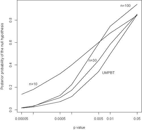
To highlight the implications of this figure, consider the curve corresponding to a sample size of n = 10 when the p-value for testing the null hypothesis of no correlation is 0.05. Based on the analysis of the OSC data, the posterior probability that the null hypothesis is true for this value of the observed correlation coefficient is 0.842. Thus, the null hypothesis is rejected at the 5% level of significance when the probability that the null hypothesis is true is approximately 84%. Other curves in Figure 4 have a similar interpretation. In general, it is clear that p-values close to 0.05 provide strong evidence in favor of the null hypothesis of no correlation, and that genuinely small p-values can occur in small samples even when the posterior probability of the null hypothesis exceeds 10%.

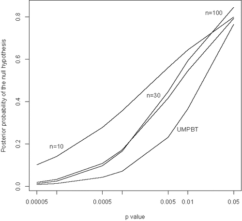
For comparison, a similar plot of posterior probabilities for the null hypothesis versus p-values based on fitting the normal model to the nonnull effect sizes is provided in Figure 5. Qualitatively, there appears to be little difference between Figures 4 and 5, suggesting that the relation between the posterior probabilities and p-values for the OSC data is not sensitive to the choice of the prior distribution chosen for the nonnull effect sizes.

Figure 5. Posterior probabilities of null hypotheses versus p-values based on the posterior means of the parameters π₀ and τ estimated from the OSC data. Similar to Figure 4, except that a normal distribution was imposed on the distribution of the nonnull effect sizes.

It is interesting to note that the posterior probabilities of null hypotheses reflected in Figure 4 are generally consistent with the empirical results reported by the OSC. For example, the OSC stated that “almost two thirds (20 of 32, 63%) of original studies with p < 0.001 had a significant p value in the replication” (OSC 2015). From the figure, the posterior probabilities of the null hypothesis when p = 0.001, based on sample sizes of 10, 30, and 100, were 0.403, 0.175, and 0.223, respectively. This suggests that approximately two-thirds of these studies report true positives and would likely replicate.

Even though it is possible to estimate the distribution of effect sizes under the alternative hypothesis using the OSC replication data, it is interesting to compare the curve labeled “UMPBT” with results that would be obtained if the distribution of effect sizes was instead generated under alternative hypotheses that produce the uniformly most powerful Bayesian tests (UMPBTs) (Johnson 2013b). The UMPBT, by definition, maximizes the probability that the Bayes factor in favor of the alternative hypothesis exceeds a given threshold. This test is anti-conservative in the sense that it is designed to make the posterior probability of the null hypothesis small so that the Bayes factor in favor the alternative hypothesis will exceed a specified threshold. That is, for a test of a given size, the UMPBT assigns minimum probability to the null hypothesis.

The posterior probabilities of null hypotheses depicted on the UMPBT curve correspond to UMPBT alternatives in which the evidence threshold was set so that the rejection region of the resulting test matched the rejection region of classical uniformly most powerful test of size 0.005.

The comparisons between p-values and posterior probabilities based on the UMPBT alternative hypotheses are qualitatively similar to the comparisons based on the distribution of effect sizes estimated from the OSC data. Both comparisons show that p-values less than 0.001 are needed to provide even weak evidence against the null hypothesis.

7. Discussion

The reanalysis of the OSC data provides an interesting new perspective on the replication rates observed in OSC (2015). Our results suggest that an effective sample size of approximately 700 hypothesis tests were conducted to generate the 73 tests that were summarized in the MA subset of studies in the OSC article. If 93% of these tests involved true null hypotheses, and each of these tests were deemed statistically significant using a 5.2% threshold, then on average these 700 tests would have generated 700 × 0.93 × 0.052 = 34 false positives. Based on the distribution of effect sizes estimated from the OSC data under the moment prior model, the average power in achieving statistical significance in 5% tests for the true alternative hypotheses was approximately 75%. On average, this implies that approximately 700 × 0.07 × 0.75 = 37 true positives would also be detected, for a total of 71 positive findings. Recall that the MA dataset contained 73 studies, of which 70 originally reported statistically significant findings.

Of the 34 false positives that would, on average, be detected from this population of 700 studies, on average only 34 × 0.052 = 2 would replicate. Among the 37 true positives, on average 37 × 0.75 = 28 would. Thus, we would expect approximately 30 of the 73 (41%) studies to replicate. This is essentially what was observed in the OSC's MA dataset. Of the 70 studies that originally reported significant findings, only 28 studies (40%) produced significant findings upon replication.

A primary conclusion that should be drawn from this reanalysis of the OSC data is that current statistical standards for declaring scientific discoveries are not sufficiently stringent to guarantee high rates of reproducibility. Indeed, p-values near 0.05 often provide substantial support in favor of a null hypothesis, and describing these values as “statistically significant” leads to unrealistic expectations regarding the likelihood that a discovery has been made. Indeed, our analysis suggests that “statistical significance” in psychology and many other social sciences should be redefined to correspond to p-values that are less than 0.005 or even 0.001 (Johnson 2013a).

Revising the standards required to declare a scientific discovery will require corresponding changes to the way science in conducted and scientific reports are interpreted. Such changes include the adoption of sequential testing methods, which are already widely used in the pharmaceutical industry to reduce costs and to quickly terminate trials that are unlikely to be successful. Early termination of trials can dramatically reduce the number of subjects required to test a theory and thus allows many more trials to be conducted.

More generally, however, editorial policies and funding criteria must adapt to higher standards for discovery. Reviewers must be encouraged to accept manuscripts on the basis of the quality of the experiments conducted, the report of outcome data, and the importance of the hypotheses tested, rather than simply on whether the experimenter was able to generate a test statistic that achieved statistical significance. This will allow researchers to publish confirmatory or contradictory findings that can be combined in meta-analyses to establish discoveries at higher levels of statistical significance. In the long run, this will result in more efficient use of resources as fewer scientists pursue research programs based on false discoveries.

Finally, we note that an inherent drawback of p-values is their failure to reflect the marginal proportion (i.e., prior probability) of tested hypotheses that are true. For this reason, we recommend the report of Bayes factors and posterior model probabilities in place of or as a supplement to p-values. These quantities have the potential for more accurately reflecting the outcome of a hypothesis test, while at the same time accounting for the prior probabilities of the null and alternative hypotheses.

Supplementary Materials

The online supplementary materials contain additional proofs.

Acknowledgments

Data analyzed in this article were obtained from the Open Science Collaboration (1). The author thanks R.C.M. van Aert for assistance in using R code supplied written in support of that article. The authors thank the associate editor and three referees for many helpful comments that significantly improved this article.

Funding

The first author's research was supported by NIH R01 CA158113.

References

- Begley, C. G., and Ellis, L. M. (2012), “Drug Development: Raise Standards for Preclinical Cancer Research,” Nature, 483, 531–533.
- Berger, J. O., and Delampady, M. (1987), “Testing Precise Hypotheses,” Statistical Science, 2, 317--335.
- Caraux, G., and Gascuel, O. (1992), “Bounds on Distributions Functions of Order Statistics for Dependent Variates,” Statistics & Probability Letters, 14, 103–105.
- Fanelli, D. (2010), ‘“Positive’ Results Increase Down the Hierarchy of the Sciences,” PLoS One, 5, e10068. doi:10.1371/journal.pone.
- Fisher, R. A. (1915), “Frequency Distribution of the Values of the Correlation Coefficient in Samples from an Indefinitely Large Population,” Biometrika, 10, 507–521.
- Francis, G. (2013), “Replication, Statistical Consistency, and Publication Bias,” (with discussion), Journal of Mathematical Psychology, 57, 153–169.
- Franco, A., Malhotra, N., and Simonovits, G. (2014), “Publication Bias in the Social Sciences: Unlocking the File Drawer,” Science, 345, 1502–1505.
- Ioannidis, J. P. (2005), “Why Most Published Research Findings are False,” PLoS Medicine, 2, e124.
- Johnson, V. E. (2004), “A Bayesian χ2 Test for Goodness-of-Fit,” Annals of Statistics, 32, 2361–2384.
- ——— (2007), “Bayesian Model Assessment using Pivotal Quantities,” Bayesian Analysis, 2, 719–733.
- ——— (2013a), “Revised Standards for Statistical Evidence,” Proceedings of the National Academy of Sciences, 110, 19313–19317.
- ——— (2013b), “Uniformly Most Powerful Bayesian Tests,” Annals of Statistics, 41, 1716--1741.
- Johnson, V. E., and Rossell, D. (2010), “On the Use of Non-Local Prior Densities in Bayesian Hypothesis Tests,” Journal of the Royal Statistical Society, Series B, 72, 143–170.
- Little, R. J., and Rubin, D. B. (2014), Statistical Analysis With Missing Data, New York: Wiley.
- McNutt, M. (2014), “Reproducibility,” Science, 343, 229–229.
- OSC (2015), “Estimating the Reproducibility of Psychological Science,” Science, 349, aac4716.
- Pashler, H., and Wagenmakers, E.-J. (2012), “Editors’ Introduction to the Special Section on Replicability in Psychological Science a Crisis of Confidence?” Perspectives on Psychological Science, 7, 528–530.
- Peplow, M. (2014), “Social Sciences Suffer from Severe Publication Bias,” Nature: News, doi:10.1038/nature.2014.15787.
- Prinz, F., Schlange, T., and Asadullah, K. (2011), “Believe it or not: How Much can we Rely on Published Data on Potential Drug Targets?” Nature Reviews Drug Discovery, 10, 712–712.
- Simmons, J., Nelson, L., and Simonsohn, U. (2011), “False-Positive Psychology: Undisclosed Flexibility in Data Collection and Analysis Allows Presenting Anything as Significant,” Psychological Science, 22, 1359–1366.
- Simonsohn, U., Nelson, L., and Simmons, J. (2014), “P-curve: A Key to the File Drawer,” Journal of Experimental Psychology: General, 143, 534–547.
- Tanner, M. A., and Wong, W. H. (1987), “The Calculation of Posterior Distributions by Data Augmentation,” Journal of the American Statistical Association, 82, 528–540.
- Wasserstein, R., and Lazar, N. (2016), “The ASA's Statement on P-Values: Context, Process, and Purpose,” The American Statistician, 70, 129--133.
- Yuan, Y., and Johnson, V. E. (2011), “Goodness-of-Fit Diagnostics for Bayesian Hierarchical Models,” Biometrics, 68, 156–164.