Bayesian Spectral Modeling for Multiple Time Series

ABSTRACT

We develop a novel Bayesian modeling approach to spectral density estimation for multiple time series. The log-periodogram distribution for each series is modeled as a mixture of Gaussian distributions with frequency-dependent weights and mean functions. The implied model for the log-spectral density is a mixture of linear mean functions with frequency-dependent weights. The mixture weights are built through successive differences of a logit-normal distribution function with frequency-dependent parameters. Building from the construction for a single spectral density, we develop a hierarchical extension for multiple time series. Specifically, we set the mean functions to be common to all spectral densities and make the weights specific to the time series through the parameters of the logit-normal distribution. In addition to accommodating flexible spectral density shapes, a practically important feature of the proposed formulation is that it allows for ready posterior simulation through a Gibbs sampler with closed form full conditional distributions for all model parameters. The modeling approach is illustrated with simulated datasets and used for spectral analysis of multichannel electroencephalographic recordings, which provides a key motivating application for the proposed methodology.

KEYWORDS:

• Gaussian mixtures
• Log-periodogram
• Markov chain Monte Carlo
• Multichannel electroencephalography
• Whittle likelihood

1 Introduction

The problem of modeling multiple time series in the spectral domain arises naturally in fields where information about frequency behavior is relevant and several signals are recorded concurrently, as in neuroscience, econometrics, and geoscience. In these fields, there is growing interest in different types of inference based on a collection of related time series. For example, multichannel electroencephalography (EEG) records measurements of electrical potential fluctuations at multiple locations on the scalp of a human subject. Identifying which locations lead to electrical brain signals with similar spectral densities and grouping them based on common spectral features is particularly meaningful, as it provides insights about the physiological state of the subject and about the spatial structure of cortical brain activity under certain experimental or clinical conditions. Therefore, developing and implementing flexible methods for spectral analysis of multiple time series is crucial in this area. It is worth emphasizing that we are considering multiple—not multivariate—time series. For a description of methods for multivariate time series in the spectral domain, refer, for example, to Shumway and Stoffer (2011).

Let $x_1,\dots ,x_n$ be n realizations from a zero-mean, weakly stationary time series $\{X_t:t=1,2,\dots \}$, with absolutely summable autocovariance function $\gamma (·)$. The spectral density function is defined as$$f(\omega )=\sum _{k=-\infty }^{+\infty }\gamma \left(k\right)\hspace{0.17em}\text{exp}\hspace{0.17em}\left(-\mathit{ik}\omega \right),\hspace{1em}\text{for}-\pi \le \omega \le \pi ,$$where $\gamma (k)=$ $\mathrm{E}(X_{t+k}{X}_t)$ denotes the autocovariance function. The standard estimator for the spectral density is the periodogram, $I_n(\omega )=$ ${\left|{\sum }_{t=1}^n{x}_t\hspace{0.17em}\text{exp}\hspace{0.17em}\left(-\mathit{it}\omega \right)\right|}^2/n$. Although $I_n(\omega )$ is defined for all $\omega \in [-\pi ,\pi ]$, it is computed at the Fourier frequencies ${\omega }_j=2\pi j/n$, for $j=0,\dots ,\lfloor n/2\rfloor$, where $\lfloor n/2\rfloor$ is the largest integer not greater than $n/2$. Because of the symmetry of the periodogram, there are only $\lfloor n/2\rfloor +1$ effective observations. Furthermore, following common practice, we exclude the observations at ${\omega }_0=0$ and ${\omega }_{\lfloor n/2\rfloor }=$ $2\pi \lfloor n/2\rfloor /n$, resulting in a sample size in the frequency domain of $N=$ $\lfloor n/2\rfloor -1$. Since the periodogram is not a consistent estimator of the spectral density, improved estimators have been obtained by smoothing the periodogram or the log-periodogram through windowing methods (e.g., Parzen 1962).

Model-based approaches to spectral density estimation are typically built from the Whittle likelihood approximation to the periodogram (Whittle 1957). For relatively large sample sizes, the periodogram realizations at the Fourier frequencies, $I_n({\omega }_j)$, can be considered independent. In addition, for large n and for zero-mean Gaussian time series, the $I_n({\omega }_j)$, for $j\ne 0,\lfloor n/2\rfloor$, are independent exponentially distributed with mean $f(\omega )$. The main advantage of the Whittle likelihood with respect to the true likelihood is that the spectral density appears explicitly and not through the autocovariance function, and the estimation problem can be cast in a regression framework with observations given by the log-periodogram ordinates and regression function defined by the log-spectral density. In particular, $\text{log}\hspace{0.17em}(I_n({\omega }_j))=$ $\text{log}\hspace{0.17em}(f({\omega }_j))+{ϵ}_j$, for $j=1,\dots ,N$, where the ${ϵ}_j$ follow a log-exponential distribution with scale parameter 1. In this context, frequentist estimation approaches include approximating the distribution of the ${ϵ}_j$ with a normal distribution and fitting a smoothing spline to the log-periodogram (Wahba 1980), and maximizing the Whittle likelihood with a roughness penalty term (Pawitan and O’Sullivan 1994). Regarding Bayesian modeling approaches: Carter and Kohn (1997) approximated the distribution of the ${ϵ}_j$ with a mixture of normal distributions and assign a smoothing prior to $\text{log}\hspace{0.17em}(f(\omega ))$; Choudhuri, Ghosal, and Roy (2004) used Bernstein polynomial priors (Petrone 1999) for the spectral density; Rosen and Stoffer (2007) expressed the log-spectral density as $\text{log}\hspace{0.17em}(f(\omega ))=$ ${\alpha }_0+{\alpha }_1\omega +h(\omega )$, with a Gaussian process prior on $h(\omega )$; and Pensky, Vidakovic, and DeCanditiis (2007) proposed Bayesian wavelet-based smoothing of the log-periodogram. More recently, Macaro and Prado (2014) extended Choudhuri, Ghosal, and Roy (2004) to consider spectral decompositions of multiple time series in designed factorial experiments, and Krafty et al. (2017) extended Rosen and Stoffer (2007) to handle replicated trivariate time series.

Here, we propose a flexible Bayesian modeling approach for multiple time series that leads to full inference of the multiple spectral densities and also allows us to identify groups of time series with similar spectral characteristics. To build a new model for a single log-spectral density, we use the Whittle approximation in the frequency domain, albeit only to the extent that the expectation of $\text{log}\hspace{0.17em}(I_n(\omega ))$ is, up to a constant, equal to $\text{log}\hspace{0.17em}(f(\omega ))$. Motivated by results in Jiang and Tanner (1999) and Norets (2010), we replace the Whittle approximation implied log-periodogram distribution with a mixture of Gaussian distributions with frequency-dependent mixture weights and mean parameters. The expectation of the Gaussian mixture distribution results in a model for the log-spectral density that can be represented as a smooth mixture of the Gaussian mean functions. The model structure for the log-spectral density is an important feature of the methodology with respect to the extension to modeling multiple spectral densities. Next, we develop a novel construction for the mixture weights which are built by consecutive differences of a logit-normal distribution function with frequency-dependent parameters. A key advantage of this construction is computational, as we can introduce normally distributed auxiliary random variables and draw from well-established posterior simulation methods for mixture models. As we extend the model to multiple time series, we set the linear functions in the mixture representation to be the same across time series, thus capturing characteristics which are shared among several spectral densities, whereas the mixture weights parameters are allowed to vary across time series, in such a way that they can select for each spectral density the appropriate mixture of mean functions. The proposed model is more parsimonious than the fully Bayesian model-based spectral estimation approaches mentioned above, leading to more efficient posterior simulation. Therefore, the methodology can be used to analyze temporal datasets that consist of a relatively large number of related time series.

Accurate estimation of spectral densities for multiple brain signals is of primary importance for neuroscience studies, which provide a key application area for our methodology. Spectral densities can appropriately summarize characteristics of brain signals recorded in various experimental or clinical settings, as documented in the literature. For instance, certain spectral characteristics of EEGs recorded from patients who received electroconvulsive therapy (ECT) as a treatment for major depression have been associated with the clinical efficacy of such treatment (Krystal, Prado, and West 1999). Also, in the area of monitoring and detection of mental fatigue, prior EEG studies have suggested an association of fatigue with an increase in the theta (4–8 Hz) band power observed in the estimated spectral of signals recorded in channels located in midline frontal scalp areas (Trejo et al. 2007).

The outline of the article is as follows. In Section 2, we describe the modeling approach, with technical details included in two appendices. In Section 3, we present results from an extensive simulation study. In Section 4, we apply the proposed model to data from multichannel EEG recordings. Finally, Section 5 concludes with a summary and discussion of possible extensions of the methodology.

2 The Modeling Approach

Here, we present the new approach to spectral modeling and inference for multiple related time series. We begin in Section 2.1 by describing the model for the log-spectral density of a single time series based on a Gaussian mixture approximation to the log-periodogram distribution. The model is then extended to multiple time series in Section 2.2.

2.1 Mixture Model Approximation to the Whittle Log-Likelihood

To motivate the modeling approach, consider the distribution of the translated log-periodogram under the Whittle likelihood. The translation constant is such that, under the Whittle approximation, the expected value of the log-periodogram is the log-spectral density. Specifically, we define $y_j=$ $\text{log}\hspace{0.17em}(I_n({\omega }_j))+\gamma$, where γ $\approx 0.57722$ is the Euler–Mascheroni constant. At the Fourier frequencies, under the Whittle likelihood approximation, the y_j are independent with the following distribution:(1) $$\begin{array}{c}{f}_Y\left(y\right)=\hspace{0.17em}\text{exp}\hspace{0.17em}\{y-\gamma -\hspace{0.17em}\text{log}\hspace{0.17em}(f(\omega ))-\hspace{0.17em}\text{exp}\hspace{0.17em}(y-\gamma -\hspace{0.17em}\text{log}\hspace{0.17em}\left(f\right(\omega \left)\right)\left)\right\},\\ \hspace{1em}\hspace{1em}y\in \mathbb{R}.\end{array}$$(1)

Therefore, $\mathrm{E}[y_j]=$ $\text{log}\hspace{0.17em}(f({\omega }_j))$ and $\text{var}[y_j]=$ ${\pi }^2/6$. Notice that the distribution in (1) is in the exponential family, and $-y_j$ are Gumbel distributed with scale parameter 1 and location parameter defined additively through $\text{log}\hspace{0.17em}(f(\omega ))$ and γ, such that the mean is $-\hspace{0.17em}\text{log}\hspace{0.17em}(f(\omega ))$. Although (1) is a standard distribution, the spectral density enters the likelihood in a nonstandard fashion through the mean parameter. Nevertheless, the Whittle approximation has been widely used in the literature because the spectral density appears explicitly in the approximate likelihood rather than through the covariance function.

We propose to replace the distribution in (1) with a structured mixture of Gaussian distributions, defined through frequency-dependent mixture weights and Gaussian mean functions. More specifically, the model on the y_j is(2) $$\begin{array}{c}{y}_j|\mathit{\theta } \stackrel{\text{ind}.}{\sim } \sum _{k=1}^K{g}_k({\omega }_j;\mathit{\xi }) \mathrm{N}(y_j|{\alpha }_k+{\beta }_k {\omega }_j/\pi ,{\sigma }^2),\\ \hspace{1em}\hspace{1em}j=1,\dots ,N,\end{array}$$(2) where $g_k({\omega }_j;\mathit{\xi })$ denotes the kth mixture weight, and $\mathit{\xi }$ is the vector of the weight parameters. The weight parameters vary depending on the specific form of the weights and will be fully specified in each case. The vector $\mathit{\theta }$ collects all model parameters, specifically, the weight parameters $\mathit{\xi }$, the intercept and slope parameters of the K mixture components means, that is, $\mathit{\alpha }=$ $\{{\alpha }_k:k=1,\dots ,K\}$ and $\mathit{\beta }=$ $\{{\beta }_k:k=1,\dots ,K\}$, and the common variance parameter ${\sigma }^2$. Note that, following common practice, we have divided ω by π, so that the normalized frequency range is (0, 1). This is done both in the Gaussian mean functions and in the weight functions, although for simpler notation we write $g_k(\omega ;\mathit{\xi })$.

Under the Whittle approximation, $\mathrm{E}[\text{log}\hspace{0.17em}(I_n(\omega ))+\gamma ]=$ $\text{log}\hspace{0.17em}(f(\omega ))$. Our approach replaces the Whittle log-periodogram distribution in (1) with the Gaussian mixture distribution in (2), and it is thus the expectation of this latter distribution that yields the log-spectral density model. (Theoretical justification for this modeling approach is discussed later in the section.) Hence, the model for the log-spectral density:(3) $$\text{log}\hspace{0.17em}\left(f\right(\omega \left)\right)=\sum _{k=1}^K{g}_k(\omega ;\mathit{\xi }) \{{\alpha }_k+{\beta }_k \omega /\pi \}, \omega \in (0,1),$$(3) that is, the log-spectral density admits a representation as a mixture of linear functions with component specific intercept and slope parameters, and with frequency-dependent weights that allow for local adjustment, and thus flexible spectral density shapes.

A key feature of the modeling approach is a novel specification for the mixture weights, which are built by consecutive differences of a distribution function on (0, 1) with frequency-dependent parameters. More specifically,(4) $$g_k(\omega ;\mathit{\xi })\equiv g_k(\mu (\omega ),\tau )={\int }_{(k-1)/K}^{k/K}{f}_Y\left(y\right|\mu (\omega ),\tau ) \mathrm{d}y,$$(4) where $f_Y(y|\mu (\omega ),\tau )$ is the density of a logit-normal distribution on (0, 1), such that the underlying normal distribution has mean $\mu (\omega )$ and precision parameter τ. Hence, at each frequency, we have a different set of weights which however evolve smoothly with the frequency. If $\mu (\omega )$ is a monotonic function in ω, the weights define a partition on the support (0, 1). We work with a linear function $\mu (\omega )=$ $\zeta +\varphi \omega /\pi$. Although other monotonic functions can be used, the linear form suffices for the theoretical results discussed below and it also facilitates posterior simulation. Parameters ζ and $\varphi$ control the modes of the weights, which in turn determine the shape of the log-spectral density. The parameter τ is a smoothness parameter, with smaller values of τ leading to smoother spectral densities. Hence, the parameters of the logit-normal distribution are interpretable and play a clear role in the shape of the weights.

The formulation for the mixture weights in (4), including the choice of the logit-normal distribution function, facilitates the implementation of a Markov chain Monte Carlo (MCMC) algorithm for posterior simulation. In particular, we can augment model (2), using continuous auxiliary variables. For each y_j, $j=1,\dots ,N$, we introduce auxiliary variable r_j, which is normally distributed with mean $\mu ({\omega }_j)=$ $\zeta +\varphi {\omega }_j/\pi$ and precision parameter τ. Then, the augmented model can be written as$$\begin{array}{c}{y}_j|r_j,\mathit{\alpha },\mathit{\beta },{\sigma }^2\stackrel{\text{ind}.}{\sim }\sum _{k=1}^K\mathrm{N}(y_j|{\alpha }_k+{\beta }_k {\omega }_j/\pi ,{\sigma }^2)\\ \hspace{1em}\times \mathbb{I}\left\{(k-1)/K<\frac{\hspace{0.17em}\text{exp}\hspace{0.17em}\left(r_j\right)}{1+\hspace{0.17em}\text{exp}\hspace{0.17em}\left(r_j\right)}\le k/K\right\},\\ r_j\left|\mathit{\xi }\stackrel{\text{ind}.}{\sim }\mathrm{N}\right(r_j|\zeta +\varphi {\omega }_j/\pi ,1/\tau ),\end{array}$$where $\mathit{\xi }=$ $(\zeta ,\varphi ,\tau )$. The full Bayesian model for a single spectral density would be completed with priors for ${\sigma }^2$ and for the elements of $\mathit{\alpha },\mathit{\beta }$, and $\mathit{\xi }$. This structure allows for a straightforward implementation of a Gibbs sampling algorithm with full conditional distributions available in closed form for all model parameters. This is demonstrated in Appendix B, in the context of the hierarchical model developed later in Section 2.2.

The Gaussian mixture model in (2), and the implied model for the log-spectral density in (3), are motivated by the theoretical results of Jiang and Tanner (1999) and Norets (2010). Jiang and Tanner (1999) showed that an exponential response distribution, involving a regression function on a finite support, can be approximated by a mixture of exponential distributions with means that depend on the covariates and with covariate-dependent mixture weights. More directly related to our model, Norets (2010) presented approximation properties of finite local mixtures of normal regressions as flexible models for conditional densities. The work in Norets (2010) focuses on the joint distribution of the response and covariates, showing that, under certain conditions, the joint distribution can be approximated in Kullback–Leibler divergence by different specifications of local finite mixtures of normals in which means, variances, and weights can depend on the covariates. Here, we consider fixed covariate values defined by the Fourier frequencies.

The key property underlying the approximation results in Jiang and Tanner (1999) and Norets (2010) is that the covariate-dependent (frequency-dependent in our context) mixture weights are such that, for some values of the weights parameters, they approximate a set of indicator functions on a fine partition of the finite support. Lemma 1 in Appendix A establishes this condition for the mixture weights defined in (4). Under this condition, it can be proved that, as the number of components increases, the approximation in (2) tends to (1) in the sense of the Kullback–Leibler divergence. Moreover, under a smoothness assumption for the log-spectral density—assuming that $\text{log}\hspace{0.17em}(f(\omega ))$ and its first and second derivatives are continuous and bounded—further theoretical justification for the model in (3) can be provided by means of results in the L_p norm for the log-spectral density; refer to the Theorem in Appendix A.

In comparison with the Bayesian inference methods for a single spectral density discussed in Section 1, we note a conceptual difference for our modeling approach. Existing methods share what may be viewed as a “semiparametric” modeling theme in that they stem from the Whittle log-periodogram distribution that includes the log-spectral density as a parameter, which is then assigned a nonparametric prior. In particular, Carter and Kohn (1997) and Rosen and Stoffer (2007) placed a smoothing spline prior on the log-spectral density, while Choudhuri, Ghosal, and Roy (2004) used a Bernstein polynomial prior for the normalized spectral density. We instead model directly the log-periodogram distribution with a mixture of Gaussian distributions with frequency-dependent weights and means. This implies the local mixture of linear functions model for the log-spectral density, which is key for our main objective, that is, flexible inference for multiple spectral densities.

Under this modeling framework, logistic weights form another class of mixture weights that satisfy the theoretical property discussed above. Such weights have the form $g_k(\omega ;\mathit{\xi })=\hspace{0.17em}\text{exp}\hspace{0.17em}\{({\zeta }_k+{\varphi }_k \omega /\pi )/\lambda \}/{\sum }_{i=1}^K\hspace{0.17em}\text{exp}\hspace{0.17em}\{({\zeta }_i+{\varphi }_i \omega /\pi )/\lambda \}$. Here, the parameter λ controls the smoothness of the transition from one subinterval of (0, 1) to another. The larger the value of λ, the smoother is the corresponding spectral density. Logistic weights have been used for spectral density estimation of a single time series in Cadonna, Kottas, and Prado (2017). Note that logistic weights are specified through a $(2K+1)$-dimensional vector $\mathit{\xi }$. Therefore, the number of parameters for models that consider these weights increases linearly with the number of components K. Moreover, the denominator in the logistic weights form complicates posterior simulation. Cadonna, Kottas, and Prado (2017) used a data augmentation step, based on auxiliary Pólya-Gamma variables (Polson, Scott, and Windle 2013), which requires N latent variables for each $k=1,\dots ,K$, thus increasing considerably the computational cost even for a single spectral density. Alternatively, the formulation for the mixture weights in (4) provides key computational advantages, as the weights are fully specified through three parameters for a single spectral density, leading to more efficient posterior simulation.

2.2 Hierarchical Model for Multiple Spectral Densities

The model for a single time series, presented in Section 2.1, was developed with a hierarchical extension in mind. Consider M related time series, which, without loss of generality, are assumed to have the same number of observations n. For example, assume that M is the number of channels located over a subject’s scalp for which we have EEG recordings. For each time series, we have N observations from the (translated) log-periodogram, which we denote as y_mj, where the first index indicates the time series ($m=1,\dots ,M$) and the second indicates the Fourier frequency ($j=1,\dots ,N$).

Now, for each m and each j we approximate the distribution of the y_mj with a smooth mixture of Gaussian distributions, as described in the previous section. We take the mean parameters of the Gaussian mixture components, that is, $({\alpha }_k,{\beta }_k)$, for $k=1,\dots ,K$, to be common among time series. This translates into a set of K linear basis functions for the log-spectral density model which are common to all time series. On the other hand, we let the parameters that specify the weights be time series specific, that is, we use the form in (4) with parameters ${\mathit{\xi }}_m=({\zeta }_m,{\varphi }_m,{\tau }_m)$, for $m=1,\dots ,M$. For each time series, the weights select the linear functions to approximate the corresponding log-spectral density. Since the spectral densities are related, similar linear basis functions can be selected for more than one location, allowing grouping of spectral densities. We use M distinct smoothness parameters τ_m to allow different levels of smoothness across the spectral densities.

Hence, extending (2), the observation stage for the hierarchical model on the M time series can be written as(5) $$y_{\mathit{mj}}|\mathit{\theta } \stackrel{\text{ind}.}{\sim } \sum _{k=1}^K{g}_k({\mu }_m\left({\omega }_j\right),{\tau }_m) \mathrm{N}(y_{\mathit{mj}}|{\alpha }_k+{\beta }_k {\omega }_j/\pi ,{\sigma }^2),$$(5) where the kth weight at the mth location is defined as in (4) in terms of increments of a logit-normal distribution function, with mean function, ${\mu }_m({\omega }_j)=$ ${\zeta }_m+{\varphi }_m {\omega }_j/\pi$, and precision parameter, τ_m, that are time series specific. Again, $\mathit{\theta }$ collects all model parameters: the intercept and slope parameters of the K mixture components means, $\mathit{\alpha }=$ $\{{\alpha }_k:k=1,\dots ,K\}$ and $\mathit{\beta }=$ $\{{\beta }_k:k=1,\dots ,K\}$, the common variance parameter ${\sigma }^2$, and the mixture weights parameters, $\mathit{\zeta }=$ $\{{\zeta }_m:m=1,\dots ,M\},\varphi =$ $\{{\varphi }_m:m=1,\dots ,M\}$, and $\mathit{\tau }=$ $\{{\tau }_m:m=1,\dots ,M\}$. Posterior simulation is implemented using the augmented version of the model based on MN normally distributed auxiliary variables, r_mj, for $m=1,\dots ,M$ and $j=1,\dots ,N$. In particular,$$\begin{array}{c}{y}_{\mathit{mj}}|r_{\mathit{mj}},\mathit{\alpha },\mathit{\beta },{\sigma }^2\stackrel{\text{ind}.}{\sim }\sum _{k=1}^K\mathrm{N}(y_{\mathit{mj}}|{\alpha }_k+{\beta }_k {\omega }_j/\pi ,{\sigma }^2)\\ \hspace{1em}\times \mathbb{I}\left\{(k-1)/K<\frac{\hspace{0.17em}\text{exp}\hspace{0.17em}\left(r_{\mathit{mj}}\right)}{1+\hspace{0.17em}\text{exp}\hspace{0.17em}\left(r_{\mathit{mj}}\right)}\le k/K\right\}\\ r_{\mathit{mj}}\left|{\mathit{\xi }}_m\stackrel{\text{ind}.}{\sim }\mathrm{N}\right(r_{\mathit{mj}}|{\zeta }_m+{\varphi }_m {\omega }_j/\pi ,1/{\tau }_m).\end{array}$$

Technical details on the Gibbs sampler used to implement the hierarchical model are given in Appendix B.

The full Bayesian model is completed with priors for $\mathit{\alpha }$, $\mathit{\beta }$, and ${\sigma }^2$, and a hierarchical prior for the $({\zeta }_m,{\varphi }_m)$ and τ_m, for $m=1,\dots ,M$. The weight parameters are assumed a priori independent of the Gaussian mixture component parameters. We assume ${\sigma }^2\sim \text{inv}-\text{gamma}(n_{{\sigma }^2},d_{{\sigma }^2})$, that is, an inverse gamma prior (with mean $d_{{\sigma }^2}/(n_{{\sigma }^2}-1)$, and $n_{{\sigma }^2}>1$), ${\alpha }_k\sim$ $\mathrm{N}({\mu }_{0\alpha },{\sigma }_{\alpha }^2)$, and ${\beta }_k\sim$ $\mathrm{N}({\mu }_{0\beta },{\sigma }_{\beta }^2)$, for $k=1,\dots ,K$. The hierarchical prior is given by$$\begin{array}{c}({\zeta }_m,{\varphi }_m)|{\mathit{\mu }}_w,{\Sigma }_w\stackrel{\text{ind}.}{\sim }\mathrm{N}({\mathit{\mu }}_w,{\Sigma }_w),\hspace{1em}m=1,\dots ,M,\\ {\tau }_m\left|d_{\tau }\stackrel{\text{ind}.}{\sim }\text{gamma}\right(n_{\tau },d_{\tau }),\hspace{1em}m=1,\dots ,M,\end{array}$$where $\text{gamma}(n,d)$ denotes the gamma distribution with mean n/d. To borrow strength across the time series, we place a bivariate normal prior on ${\mathit{\mu }}_w$, and an inverse Wishart prior on the covariance matrix Σ_w. For the τ_m, we fix the shape parameter, $n_{\tau }$, and place a gamma prior on the rate parameter, $d_{\tau }$.

The prior on the intercept parameters, α_k, summarizes information about the spectral density value near ω = 0, while the prior on the slope parameters, β_k, can be used to express beliefs about the shape of the spectral density. For instance, for multimodal spectral densities, we expect some selected β_k to be positive and some negative, whereas for unimodal spectral densities, we expect all the selected β_k to have the same sign. The parameters ζ_m and ${\varphi }_m$, for $m=1,\dots ,M$, determine the location of the modes of the weights corresponding to the mth spectral density, while the τ_m are smoothness parameters with smaller values favoring smoother spectral densities. Given the model structure that involves common parameters for the mixture components, inferences for the $({\zeta }_m,{\varphi }_m)$ are useful in identifying groups of time series with similar spectral characteristics. This is demonstrated with the data illustrations of Sections 3 and 4.

In this work, the number of mixture components, K, is fixed. The modeling approach can be generalized to a random K, albeit at the substantial expense of a more computationally challenging posterior simulation method. There is a growing literature on the roles of the total number of mixture components, K, and the number of effective (active) components, $\tilde{K}\le K$, in finite mixture models and nonparametric mixture models (e.g., Miller and Harrison 2018). Our modeling approach is based on smooth mixtures in which both mixture weights and means depend on a covariate (the frequency in our case). To our knowledge, there is no literature that provides a comprehensive study on the role of K and $\tilde{K}$ in smooth mixtures. The values of the weight parameters, together with K, determine how many components, $\tilde{K}\le K$, are effectively used by the model. Because of the smoothness, different subsets of the support can have a different number of components which are “practically” different from zero. Here, we consider $\tilde{K}$ as the number of components which are (essentially) not equal to zero over the entire support.

Based on extensive empirical investigation with several datasets, including the ones in Section 3, we have observed that, in general, a relatively small number of mixture components suffices to capture different spectral density shapes, with inference results being robust to the choice of K. For instance, for the synthetic data from an AR(2) process with modulus 0.95 and frequency 2.07 (first set of time series for the simulation scenario of Section 3.2), point and interval estimates for the log-spectral density were essentially identical for K = 20, 30, 50. Moreover, the posterior distribution for $\tilde{K}$ concentrated most of its probability mass on values from 5 to 8 (the posterior mode being at 6), and, importantly, this distribution was largely unaffected under K = 30 and K = 50.

3 Simulation Study

In order to assess the performance of the proposed modeling approach, we designed three different data generating mechanisms that represent three hypothetical scenarios involving multiple related time series. In each scenario, we have M = 15 time series. Moreover, we consider replicates, meaning that more than one time series is generated from the same underlying process. (Although results are not shown, we also considered a setting involving M = 5 time series mutually different from each other, two AR(1) processes, two AR(2) processes, and white noise. The model captured successfully the different spectral density shapes, albeit, as expected, with wider posterior uncertainty bands than the ones reported here.) For each time series, we simulated n = 300 time points, leading to N = 149 observations from the log-periodogram. In addition to posterior estimates and credible intervals for the spectral densities, we investigate the posterior distribution of the weight parameters, ζ_m, ${\varphi }_m$, and τ_m, for $m=1,\dots ,M$, which can be useful in identifying similar spectral characteristics across multiple time series.

To evaluate differences between two spectral densities, we use the concept of total variation distance (TVD) for normalized spectral densities. The total variation is a distance measure for probability distributions and it has been used to quantify the distance between two spectral densities, after normalization (e.g., Euan, Ombao, and Ortega 2015). In particular, the TVD between two normalized spectral densities $f^{*}=$ $f/{\int }_{\Omega }f(\omega )\mathrm{d}\omega$ and $g^{*}=$ $g/{\int }_{\Omega }g(\omega )\mathrm{d}\omega$, where $\Omega =(0,\pi )$, is defined as $\text{TVD}(f^{*},g^{*})=$ $1-{\int }_{\Omega }\min \{f^{*}(\omega ),g^{*}(\omega )\}\mathrm{d}\omega$. This is equivalent to half of the L₁ distance between $f^{*}$ and $g^{*}$, that is, $\text{TVD}(f^{*},g^{*})=$ $\left|\right|f^{*}-g^{*}|{|}_1/2$. We use the TVD as a measure of discrepancy between spectral densities because it is symmetric and bounded between 0 and 1, with the value of 1 corresponding to the largest possible distance between the normalized spectral densities. Moreover, it can be proved that if $\text{log}\hspace{0.17em}{f}_k\stackrel{L_p(0,\pi )}{\to }\hspace{0.17em}\text{log}\hspace{0.17em}f$, then $f_k/\int f_k(\omega )\mathrm{d}\omega \stackrel{\text{TVD}}{\to }f/\int f(\omega )\mathrm{d}\omega$ (see Lemma 2 in Appendix A). Under a Bayesian modeling approach, we have a posterior distribution for the TVD of any two given spectral densities. We use the posterior distributions of the TVDs to compare the inferred spectral densities of multiple time series, as illustrated in the analyses of simulated and real data shown below.

3.1 First Scenario

The goal of this simulated scenario is to evaluate the performance of our model for time series with monotonic spectral densities, and also to test if the model is able to recognize white noise. In order to compare our posterior estimates to the true spectral densities, we simulated data from processes with spectral densities available in analytical form. We considered three underlying generating processes, with five replicates in each case, leading to a total of M = 15 time series. The first five time series were generated from an autoregressive process of order one, or AR(1) process, with parameter 0.9. The next five time series (labeled from 6 to 10) were generated from an AR(1) process with parameter 0.5. Finally, the last five time series were generated from pure white noise, or equivalently an AR(1) process with parameter 0. Hence, the underlying spectral densities for the first two groups are monotonic decreasing. The spectral density corresponding to the first five time series has a larger slope and is less noisy, while the one corresponding to the second group has smaller slope and more variability in the periodogram realizations. The spectral density for the last five time series is a constant at one, that corresponds to the variance of the white noise.

We fixed the number of mixture components to K = 30; similar results were obtained with a larger value of K. We assumed α_k and β_k to be independent normally distributed centered at zero with variance 1000 such that the linear basis can have a wide range of motion. For the common variance parameters, we used an inverse gamma prior with mean 3 and variance 9. For the smoothness parameters τ_m, $m=1,\dots ,M$, we fixed the shape parameter to 30 and placed a $\text{gamma}(3,20)$ on the rate parameter. This results in a marginal prior distribution for each τ_m that supports a large interval on the positive real line. Moreover, since each time series has its own smoothness parameter, we can have different levels of smoothness for different spectral densities. The hyper-prior on the mean parameter was centered at 0 and had variance 10, while the Inverse Wishart distribution parameters were chosen in a way that the marginal distributions for the diagonal elements were $\text{inv}-\text{gamma}(3,3)$, and the implied prior distribution on the correlation between ζ_m and ${\varphi }_m$ was diffuse on (0, 1).

Figure 1 shows the joint posterior densities for $({\zeta }_m,{\varphi }_m)$ (top left panel) and the prior and posterior densities for τ_m (top right panel) for $m=1,\dots ,M$. The color red corresponds to the first five time series, the blue to the time series from sixth to tenth, and the green one to the last five time series. Clearly, the joint posterior distribution of $({\zeta }_m,{\varphi }_m)$ allows us to accurately identify the three groups. In addition, we notice that there is a pattern in the posterior distribution: the steeper the slope of the spectral density (i.e., the larger the AR coefficient), the larger the value of ${\zeta }_m/{\varphi }_m$, which determines the shape of the posterior spectral density estimates. The posterior distributions of the τ_m parameters that determine the smoothness of the spectral densities do not show a clear distinction among the three groups. Figure 1 (bottom panel) shows the posterior distributions of the TVDs with respect to the true white noise spectral density. As expected, the distances for the time series in the third group are the smallest. In addition, the TVD results support the clustering among the spectral densities identified through the posterior distribution of the $({\zeta }_m,{\varphi }_m)$. 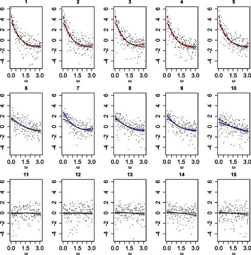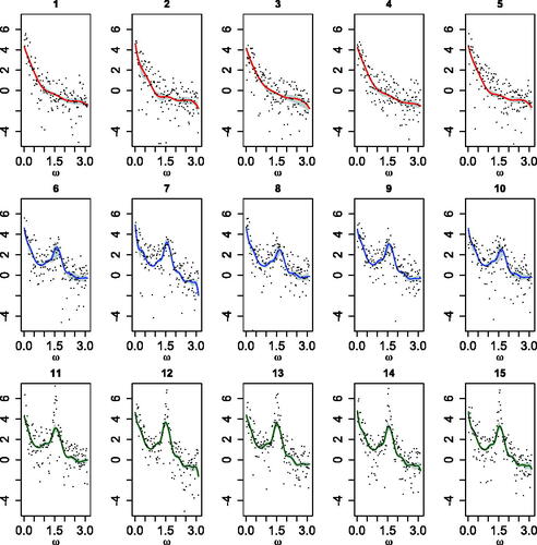Figure 2 shows the true log-spectral densities, as well as the corresponding posterior mean estimates and 95% credible intervals. The model adequately captures the different log-spectral density shapes and is successful in discerning noisy processes with corresponding monotonic spectral densities from pure white noise processes.

Fig. 1 First simulation scenario. Joint posterior densities for $({\zeta }_m,{\varphi }_m)$ (top left panel), marginal prior density (dashed line) and posterior densities for τ_m (top right panel), for $m=1,\dots ,M$, and boxplots of posterior samples for the TVD of each estimated spectral density from the white noise spectral density (bottom panel).

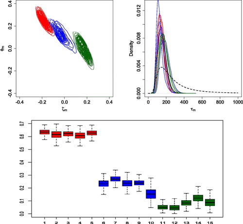
Fig. 2 First simulation scenario. Posterior mean estimates (solid lines) and 95% credible intervals (shaded regions) for each log-spectral density. Each panel includes also the true log-spectral density (dashed line) and the log-periodogram (dots).

3.2 Second Scenario

The first scenario dealt with monotonic spectral densities. Here, we test model performance in the case of multiple unimodal spectral densities. A unimodal spectral density shows a single major peak at a particular frequency. For example, processes with corresponding unimodal spectral densities are second-order quasi-periodic autoregressive processes with one dominating frequency. We generated a set of M = 15 time series from two different AR(2) processes. The first eight time series were simulated from an AR(2) process with modulus 0.95 and frequency $\omega =2.07,$ while the last seven time series were simulated from an AR(2) process with the same modulus of 0.95 but with frequency $\omega =1.08$. Hence, the time series contain essentially the same amount of information (the modulus was 0.95 in both groups) and have a single quasi-periodic component, with dominating frequency $\omega =2.07$ for the first group, and $\omega =1.08$ for the second group.

We applied again the model with K = 30 components, and with the same prior specification used in the first scenario for all parameters, except for the hyperparameter that controls the smoothness of the estimates. Since we expect less smooth spectral densities than the first scenario, we fix the shape parameter of the gamma prior on τ_m to 60 for all m, and place a $\text{gamma}(10,300)$ hyperprior on the rate parameter. This results in a marginal prior distribution for the τ_m that has support on relatively large values.

Figure 3 shows the joint posterior densities for $({\zeta }_m,{\varphi }_m)$ (left panel) and the posterior densities for τ_m (right panel), together with the prior marginal density for τ_m, for $m=1,\dots ,M$. The color red corresponds to the first eight time series and the blue to the last seven time series. 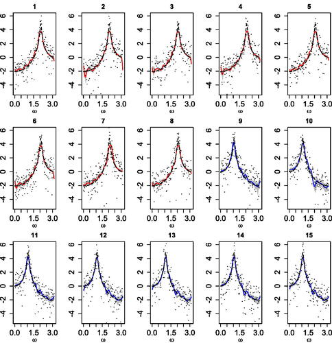Since parameters $({\zeta }_m,{\varphi }_m)$ determine the location of the peak for each time series, the posterior densities of $({\zeta }_m,{\varphi }_m)$ show a clear separation of the parameters relative to the two groups. The posterior densities of the τ_m parameters are similar for all the time series, as expected, since the peak has the same amplitude. Figure 4 shows the posterior mean estimates and 95% credible intervals for the log-spectral densities. The log-periodograms and true log-spectral densities are also shown. Our model adequately captures the distinct log-spectral density shapes and successfully identifies the peaks of the quasi-periodic components for the two types of processes.

Fig. 3 Second simulation scenario. Joint posterior densities for $({\zeta }_m,{\varphi }_m)$ (left panel) and for τ_m (right panel), for $m=1,\dots ,M$. The right panel includes also the marginal prior density (dashed line) for the τ_m.

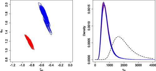
Fig. 4 Second simulation scenario. Posterior mean estimates (solid lines) and 95% credible intervals (shaded regions) for each log-spectral density. Each panel includes also the true log-spectral density (dashed line) and the log-periodogram (dots).

3.3 Third Scenario

In this scenario, all M = 15 simulated time series share an underlying first-order autoregressive component, and some of them present an additional second-order autoregressive component. Specifically, the first five time series were simulated from an AR(1) with parameter 0.9. The next five time series were simulated from a sum of two autoregressive processes, an AR(1) and an AR(2). The AR(1) process has parameter 0.9, as in the previous set of time series, while the AR(2) process was assumed to be quasi-periodic, with modulus 0.83 and argument $\omega =1.54$. The last five time series were again simulated from a sum of an AR(1) process and an AR(2) process. The AR(1) process has parameter 0.9 as before, whereas the AR(2) was a quasi-periodic process with modulus 0.97 and argument $\omega =1.54$. In the second and third groups, the spectral densities show an initial decreasing shape and a peak corresponding to the argument $\omega =1.54$. While the argument is the same, the modulus is larger in the third group, hence the peak is more pronounced.

We applied the model with K = 30 mixture components, using the same prior specification as in the second scenario, because we expected similar smoothness for the spectral densities. Figure 5 shows the joint posterior densities for $({\zeta }_m,{\varphi }_m)$ (top left panel) and the posterior densities for τ_m (top right panel), for $m=1,\dots ,M$. The color red identifies the first five time series, the blue the time series from sixth to tenth, and the green the last five time series. The posterior distributions for $({\zeta }_m,{\varphi }_m)$ cluster into two groups, the time series corresponding to the AR(1) process and the time series corresponding to the sum of AR(1) and AR(2) processes. However, as expected, it is hard to differentiate between the two groups of time series generated from the sum of AR(1) and AR(2) processes, because they share the same periodicities, with only the moduli being different. The boxplots in Figure 5 summarize the posterior distributions of the total variation distances between the estimates and the spectral density of an AR(1) model with parameter 0.9, which corresponds to the true spectral density for the first set of five time series. As expected, the posterior distribution of the total variation distance for the first five time series is concentrated around smaller values. Also as expected, there is no clear distinction between the second and the third group. Figure 6 displays the posterior mean estimates and 95% credible intervals for the log-spectral densities. As with the previous simulation examples, the model successfully recovers the different spectral density shapes and identifies the peak of the quasi-periodic component for the last ten time series.

Fig. 5 Third simulation scenario. Joint posterior densities for $({\zeta }_m,{\varphi }_m)$ (top left panel), marginal prior density (dashed line) and posterior densities for τ_m (top right panel), for $m=1,\dots ,M$, and boxplots of posterior samples for the total variation distance of each estimated spectral density from the AR(1) spectral density (bottom panel).

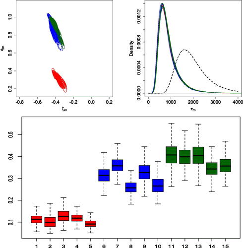
Fig. 6 Third simulation scenario. Posterior mean estimates (solid lines) and 95% credible intervals (shaded regions) for each log-spectral density. Each panel includes also the log-periodogram (dots).

4 Application: Electroencephalogram Data

Multichannel EEG recordings arise from simultaneous measurements of electrical fluctuations induced by neuronal activity in the brain, using electrodes placed at multiple sites on a subject’s scalp. One application area in which EEG recordings have proved very useful is the study of brain seizures induced by ECT as a treatment for major depression. The time series studied here are part of a more extensive study. Further details and data analyses can be found in West, Prado, and Krystal (1999) and Krystal, Prado, and West (1999). EEGs were recorded at 19 locations over the scalp of one subject that received ECT. The original sampling rate was 256 Hz. We consider first 300 observations from a mid-seizure portion, after subsampling the electroencephalogram signals every sixth observation. We refer to this dataset as ECT data 1.

We applied our model to these 19 time series, using K = 50 mixture components. Similar results were obtained using a larger number of components. The priors on the parameters were defined as in the second and third simulated scenarios above. Figure 7 shows the joint posterior densities for $({\zeta }_m,{\varphi }_m)$, for the 19 channels. The configuration of the plots shown in the figure aims to provide a schematic representation of the physical location of the electrodes over the subject’s scalp. For example, the first row of the plots represents the frontmost electrodes on the patient’s scalp (F${}_{p_1}$ and F${}_{p_2}$) viewed from above. Overall, there is no clear distinction of the posterior distributions among the various channels. However, in certain regions of the brain the posterior distributions of the $({\zeta }_m,{\varphi }_m)$ are concentrated around values similar to the those obtained from locations in that same region (e.g., channels C${}_z,$ P${}_z,$ P₃, and C₃). On the other hand, some channels that are next to each other show differences in their posterior distributions (e.g., C_z and C₄). Figure 8 shows the posterior mean estimates and the corresponding 95% posterior credible intervals for the spectral densities along with the log-periodograms. All the channels show a peak around 3.3–3.5 Hz for these series taken from the central portion of the EEG signals. These results are consistent with previous analyses which indicate that the observed quasi-periodicity is dominated by activity in the delta frequency range, that is, in the range from 1 to 5 Hz (West, Prado, and Krystal 1999; Prado, West, and Krystal 2001). The peak is slightly shifted to the left in the temporal channels with respect to the frontal channels. This aspect is also consistent with previous analyses. To quantify the differences among spectral densities, we chose to compare each density to the one in the central channel, C${}_z,$ as this channel has been used as a reference channel in previous analyses (Prado, West, and Krystal 2001). Figure 9 shows the posterior distributions of the TVDs between the spectral density estimates at each channel and that for the reference channel C_z. We can clearly see a correspondence between the posterior distribution of the weight parameters and the spectral density estimates. Figures 7 and 9 suggest that channels P${}_3,$ P${}_z,$ C${}_3,$ are the ones that share the most similar spectral features with channel C_z.

Fig. 7 ECT data 1. Joint posterior densities for $({\zeta }_m,{\varphi }_m),m=1,\dots ,19$.

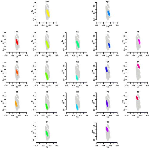
Fig. 8 ECT data 1. Posterior mean estimates (solid lines) and 95% credible intervals (shaded regions) for the log-spectral densities corresponding to the 19 channels. Each panel includes also the log-periodogram (dots) from the specific channel.

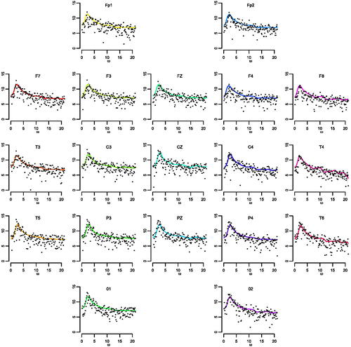
Fig. 9 ECT data 1. Boxplots of posterior samples for the total variation distances between the spectral densities for each channel and the spectral density of the reference channel C_z.

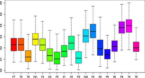
The analysis above shows that, although there are some differences across the time series recorded at different locations for the same time period, all the locations share similar features with respect to the location of the peak in their estimated log-spectral densities. We now show that our method can effectively capture differences in the spectral content of EEG time series that were recorded during different time periods over the course of the ECT induced seizure. To this end, we use the same dataset described above, but analyze time series recorded only in five channels, specifically, channels C${}_3,$ F${}_z,$ C${}_z,$ P_z, and C₄, at three different temporal intervals (we refer to this dataset as ECT data 2). The first temporal interval corresponds to the beginning of the seizure, the second one is the interval considered in the previous analysis which corresponds to a mid-seizure period, while the third one was recorded later in time, when the seizure was fading. We emphasize that this is only an illustrative example to study if our method is able to capture different spectral characteristics in multiple EEGs. This is not the ideal model for this more general data structure, as we are not taking into account the fact that we have three different time periods. We analyze the 15 EEGs corresponding to five channels for three different time periods, using the model with K = 50 mixture components and the same prior specification described above. Figure 10 shows the joint posterior densities for $({\zeta }_m,{\varphi }_m)$ and τ_m, for the 15 time series. The five series in the first time period (plotted in red color) are essentially indistinguishable in terms of the distributions of $({\zeta }_m,{\varphi }_m)$, while the series that correspond to mid (blue color) and later (green color) portions of the induced seizure display more variability. Figure 11 shows the posterior mean estimates of the log-spectral densities and the corresponding 95% posterior credible intervals along with the log-periodograms. In this case, there is a clear distinction in the posterior distributions of the time series corresponding to different time periods. In fact, the peak in the log-spectral density is more pronounced for those series that correspond to the beginning of the seizure. The peak shifts to the left and its power decreases in the successive time periods. In particular, in the last time period, the power of the peaks is the lowest and the variability in the log-periodogram observations and the estimated log-spectral densities is larger. There is also an increase of spectral variability over the time periods. These findings are consistent with previous analyses of these data, using nonstationary time-varying AR models (West, Prado, and Krystal 1999; Prado, West, and Krystal 2001).

Fig. 10 ECT data 2. Joint posterior densities for $({\zeta }_m,{\varphi }_m)$ (left panel) and τ_m (right panel), for $m=1,\dots ,15$. The right panel includes also the marginal prior density (dashed line) for the τ_m.

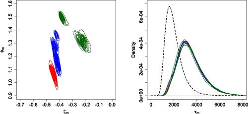
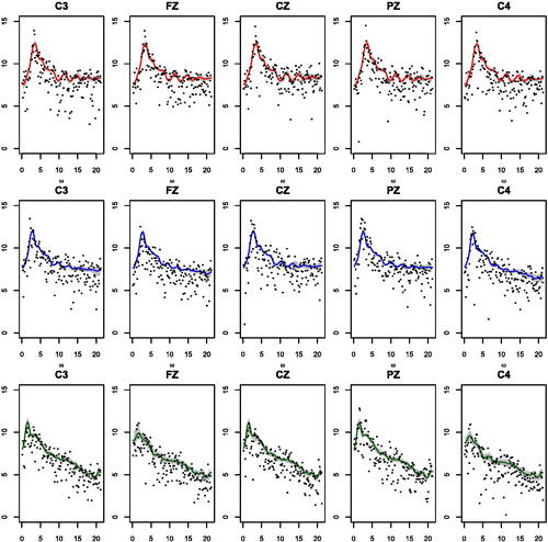
Fig. 11 ECT data 2. Log-periodograms (dots), posterior mean estimates (solid lines), and 95% credible intervals (shaded regions) for the log-spectral densities corresponding to the 15 time series obtained from five channels for three time periods: beginning of the seizure (top row), mid-seizure (middle row), and end of the seizure (bottom row).

5 Discussion

We have developed methodology for the analysis and estimation of multiple time series in the spectral domain. We note again that the methodology is developed for multiple, not multivariate, time series. This is a problem receiving some attention in the recent literature, but there is generally a shortage of Bayesian methods that deal jointly and efficiently with multiple time series in the spectral domain. Methods for multivariate time series analysis are available, but often have the drawback of high computational cost, and are applicable in practice to a limited number of dimensions (rarely higher that 2–3). Our approach is based on replacing the Whittle approximation implied log-periodogram distribution with a mixture of Gaussian distributions with frequency-dependent weights and mean functions, which results in a flexible mixture model for the corresponding log-spectral density. The main idea for a single unidimensional time series was presented in Cadonna, Kottas, and Prado (2017), where logistic weights were used. Here, the mixture weights are built through differences of a distribution function, resulting in a substantially more parsimonious specification than logistic mixture weights. This is a fundamental feature of the proposed model, as it naturally leads to a hierarchical extension that allows us to efficiently consider multiple time series and borrow strength across them. As an additional advantage, casting the spectral density estimation problem in a mixture modeling framework allows for relatively straightforward implementation of a Gibbs sampler for inference. The proposed modeling approach is parsimonious without sacrificing flexibility. Through simulation studies, we have demonstrated the ability of the model to uncover both monotonic and multimodal spectral density shapes, as well as white noise. We also applied the methodology to multichannel EEG recordings, obtaining results that are in agreement with neuroscientists’ understanding.

The Whittle likelihood is exact only for Gaussian white noise, but leads to asymptotically correct estimation for both Gaussian and non-Gaussian time series (e.g., Hannan 1973). However, Whittle likelihood based estimation may result in loss of efficiency for small sample sizes, both for non-Gaussian time series and for highly autocorrelated Gaussian time series (e.g., Contreras-Cristan, Gutierrez-Pena, and Walker 2006). The Whittle approximation involves an assumption of asymptotic independence between Fourier coefficients, as well as the assumption of a stationary Gaussian time series. To relax the former assumption, Kirch et al. (2017) propose a nonparametric correction, based on Bernstein polynomial priors, of a parametric likelihood (focusing on AR(p) models for the parametric likelihood).

Our methodology relies on the asymptotic independence of the $I_n({\omega }_j)$, but uses the Whittle log-periodogram distribution only to the extent that $\mathrm{E}[\text{log}\hspace{0.17em}(I_n(\omega ))]$ is asymptotically equal to $\text{log}\hspace{0.17em}(f(\omega ))-\gamma$. Hence, it has the potential to enhance the scope of Whittle likelihood based inference for non-Gaussian time series. Such potential can be further explored through models that build from the assumption $\mathrm{E}[I_n(\omega )]=$ $f(\omega )$, which holds asymptotically for zero-mean, weakly stationary time series. In the context of our modeling framework, we would now seek mixture models (again, with frequency-dependent mixture weights and kernel component parameters) directly for the periodogram distribution. Then, the expectation of the mixture distribution would provide the spectral density model. Here, the choice of the mixture kernel and/or mixture weights would need to balance desirable theoretical results for the mixture distribution and its expectation with appropriate structure for the implied spectral density that corresponds to specific classes of time series. In particular, as suggested by a reviewer, it will be of interest to extend the approach to model spectral densities for long-range dependent time series, for which existing Bayesian methods include Liseo, Marinucci, and Petrella (2001) and Chopin, Rousseau, and Liseo (2013).

Extending the methodology for nonstationary time series is another interesting direction. As the last ECT example shows the frequency content is different in the different time intervals. Ideally, we would like to have a model that allows us to infer time-varying spectral characteristics in multiple time series. Classical spectral analysis is based on the assumption of weak stationarity. Such an assumption is often not satisfied, especially when we need to analyze long time series, and the covariance properties vary over time. This is equivalent to saying that the distribution of power over frequency changes as time evolves. Future research will focus on expanding our hierarchical spectral model in such a way that the evolution of the spectral content over time can also be included, with the goal of estimating time-varying spectral densities.

Acknowledgments

The authors thank an Associate Editor and two reviewers for several useful comments.

Additional information

Funding

This work is part of the Ph.D. dissertation of the first author, completed at University of California, Santa Cruz. The research was supported in part by the National Science Foundation under awards DMS 1407838 and SES 1461497.

Appendix A

Theoretical Results

For simpler notation, and without loss of generality, we consider from the outset the normalized frequency range, such that $\omega \in$ $\Omega =(0,1)$. However, the results are valid for any bounded interval on the real line. We show that a smooth function h on $\Omega =(0,1)$ can be approximated by a local mixture of linear functions, $h_K(\omega )=$ ${\sum }_{k=1}^K{g}_k(\mu (\omega ),\tau )\{{\alpha }_k+{\beta }_k\omega \}$, with weights$$g_k(\mu (\omega ),\tau )=\frac{1}{\sqrt{2\pi }}{\int }_{(b_{k-1}-\mu (\omega \left)\right)\sqrt{\tau }}^{(b_k-\mu (\omega \left)\right)\sqrt{\tau }}\hspace{0.17em}\text{exp}\hspace{0.17em}(-x^2/2) \mathrm{d}x,$$with $b_k=$ $\text{log}\hspace{0.17em}\{k/(K-k)\},b_{k-1}=$ $\text{log}\hspace{0.17em}\{(k-1)/(K-k+1)\}$, and $\mu (\omega )=$ $\zeta +\varphi \omega$.

Let ${\Vert f\Vert }_p=$ ${\left({\int }_0^1|f(\omega ){|}^p\mathrm{d}P(\omega )\right)}^{\frac{1}{p}}$ denote the L_p norm, where P is an absolutely continuous distribution on Ω. Moreover, denote by χ_B the indicator function for $B\subseteq \Omega$. Let a and b be two integers, with b > a, and define the partition $\{Q_{a+1},\dots ,Q_b\}$ of $\Omega =(0,1)$, with $Q_{a+1}=$ $\left(0,\frac{1}{b-a}\right)$ and $Q_k=$ $\left[\frac{k-a-1}{b-a},\frac{k-a}{b-a}\right)$, for $k=a+2,\dots ,b$. Each element of the partition has length $1/(b-a)$. The following lemma is used to obtain the main result.

Lemma 1

. Let $g_k(\mu (\omega ),\tau )$ be the kth weight as defined in (A.1). Then, there exist values for ζ and $\varphi$, and integers k₁ and k₂, with $k_2>k_1$, such that, for $k=k_1+1,\dots ,k_2$, $\underset{\tau \to \infty }{\lim }\left|\right|g_k-{\chi }_{Q_k}|{|}_p=0$, for any $p\in \mathbb{N}$. Moreover, for $1<k\le k_1$ or $k_2<k\le K$, $\underset{\tau \to \infty }{\lim }\left|\right|g_k|{|}_p=0$, for any $p\in \mathbb{N}$.

Proof.

Based on the form of the mixture weights in (A.1), for any fixed ω, and for any $k=1,\dots ,K$, we have$$\underset{\tau \to \infty }{\lim }{g}_k(\mu (\omega ),\tau ) \hspace{1em}=\{\begin{array}{cc}\hfill & 1\hspace{1em}\hspace{1em}\hspace{0.17em}\text{log}\hspace{0.17em}\left(\frac{k-1}{K-k+1}\right)\le \mu (\omega )<\hspace{0.17em}\text{log}\hspace{0.17em}\left(\frac{k}{K-k}\right)\hfill \\ \hfill & 0\hspace{1em}\hspace{1em} \mathrm{o}.\mathrm{w}.\hfill \end{array}$$

and thus$$\underset{\tau \to \infty }{\lim }{g}_k(\mu (\omega ),\tau )=\{\begin{array}{cc}\hfill & 1\hspace{1em}\hspace{1em}\frac{k-1}{K}\le \frac{\hspace{0.17em}\text{exp}\hspace{0.17em}(\mu (\omega \left)\right)}{1+\hspace{0.17em}\text{exp}\hspace{0.17em}(\mu (\omega \left)\right)}<\frac{k}{K}\hfill \\ \hfill & 0\hspace{1em}\hspace{1em} \mathrm{o}.\mathrm{w}.\hfill \end{array}$$

We can find values of ζ and $\varphi >0$, and integers k₁ and k₂, with $k_2>k_1$, such that $\text{exp}\hspace{0.17em}(\mu (0))/\{1+\hspace{0.17em}\text{exp}\hspace{0.17em}(\mu (0))\}=$ $k_1/K$ and $\text{exp}\hspace{0.17em}(\mu (1))/\{1+\hspace{0.17em}\text{exp}\hspace{0.17em}(\mu (1))\}=$ $k_2/K$, and such that we can build a linear approximation of $\text{exp}\hspace{0.17em}(\mu (\omega ))/\{1+\hspace{0.17em}\text{exp}\hspace{0.17em}(\mu (\omega ))\}$, specifically, given by $(k_1/K)+\{(k_2-k_1)/K\}\omega$. Therefore, the partition induced on Ω is $\{(0,1/(k_2-k_1)),$ $[1/(k_2-k_1),2/(k_2-k_1)),\dots ,$ $[(k_2-k_1-1)/(k_2-k_1),1)\}$. From the limiting result above, for $k=k_1+1,\dots ,k_2$, we have $g_k(\mu (\omega ),\tau )\to {\chi }_{Q_k}(\omega )$, almost surely, as $\tau \to \infty$. In addition, for $0<k\le k_1$ or $k_2<k\le K$, $g_k(\mu (\omega ),\tau )\to 0$, almost surely, as $\tau \to \infty$. Moreover, for $k=k_1+1,\dots ,k_2$, $|g_k(\mu (\omega ),\tau )-{\chi }_{Q_k}(\omega ){|}^p\le 1$, for $\omega \in (0,1)$, and for $0<k\le k_1$ or $k_2<k\le K$, $|g_k(\mu (\omega ),\tau ){|}^p\le 1$, for $\omega \in (0,1)$. Hence, from the dominated convergence theorem, for $k=k_1+1,\dots ,k_2$, $\underset{\tau \to \infty }{\lim }\left|\right|g_k-{\chi }_{Q_k}|{|}_p=0$, for any $p\in \mathbb{N}$. Finally, for $1<k\le k_1$ or $k_2<k\le K$, we have that $\underset{\tau \to \infty }{\lim }\left|\right|g_k|{|}_p=0$, for any $p\in \mathbb{N}$. □

Based on Lemma 1, the local mixture weights approximate the set of indicator functions on the partition $\{Q_{k_1+1},\dots ,Q_{k_2}\}$, for any fixed K, k₁ and k₂, with $k_2>k_1$. The following result establishes that the distance in the L_p norm between the target log-spectral density, h, and the proposed mixture model h_K is bounded by a constant that is inversely proportional to the square of $K^{*}=k_2-k_1<K$.

Theorem.

Let $h\in W_{2,K_0}^{\infty }$, that is, the Sobolev space of continuous functions bounded by K₀, with the first two derivatives continuous and bounded by K₀. Then, $\underset{h_K}{\inf }{\Vert h_K-h\Vert }_p\le K_0/(2K^{*}{}^2)$.

Proof.

We start by proving that, for fixed K, k₁ and k₂, with $k_2>k_1$, any $h\in W_{2,K_0}^{\infty }$ can be approximated by a piecewise linear function on the partition $\{Q_{k_1+1},\dots ,Q_{k_2}\}$, with the L_p distance bounded by a constant that depends on $K^{*}=k_2-k_1$. For each interval Q_k, $k=k_1+1,\dots ,k_2$, consider a point ${\omega }_k^{*}\in Q_k$ and the linear approximation based on the first-order Taylor series expansion: ${\widehat{h}}_k(\omega )=$ ${\widehat{\alpha }}_k+{\widehat{\beta }}_k\omega$, for $\omega \in Q_k$, where ${\widehat{\alpha }}_k$ $=h({\omega }_k^{*})-{\omega }_k^{*}{h}^{\prime }({\omega }_k^{*})$ and ${\widehat{\beta }}_k=h^{\prime }({\omega }_k^{*})$; here, $h^{\prime }({\omega }_k^{*})$ denotes the first derivative of $h(\omega )$ evaluated at ${\omega }_k^{*}$, with similar notation used below for the second derivative. We have ${\Vert \left\{{\sum }_{k=k_1+1}^{k_2}{\chi }_{Q_k}{\widehat{h}}_k\right\}-h\Vert }_p$ $={\Vert {\sum }_{k=k_1+1}^{k_2}{\chi }_{Q_k}\left\{{\widehat{h}}_k-h\right\}\Vert }_p\le$ $\underset{k_1+1\le k\le k_2}{\sup }{\Vert {\widehat{h}}_k-h\Vert }_{\infty }$, where ${\Vert \Vert }_{\infty }$ denotes the $L_{\infty }$ norm. Now, for each interval Q_k, we consider the second-order expansion of h around the same ${\omega }_k^{*}\in Q_k$. Note that the partition $\{Q_{k_1+1},\dots ,Q_{k_2}\}$ satisfies the property that, for any k, and for any ω₁ and ω₂ in Q_k, $|{\omega }_1-{\omega }_2|\le 1/K^{*}$. Using this property and the fact that the second derivative of h is bounded by K₀, we obtain $|{\widehat{h}}_k(\omega )-h(\omega )|\le$ $|0.5{(\omega -{\omega }_k^{*})}^2{h}^{″}({\omega }_k^{*})|\le$ $K_0/(2K^{*}{}^2)$. Therefore, ${\Vert \left\{{\sum }_{k=k_1+1}^{k_2}{\chi }_{Q_k}{\widehat{h}}_k\right\}-h\Vert }_p\le K_0/(2K^{*}{}^2)$. Using the triangular inequality, we can write$$\begin{array}{c}{\Vert \left\{\sum _{k=k_1+1}^{k_2}{g}_k{\widehat{h}}_k\right\}-h\Vert }_p\le {\Vert \sum _{k=k_1+1}^{k_2}\left\{g_k-{\chi }_{Q_k}\right\}{\widehat{h}}_k\Vert }_p\\ \hspace{1em}+{\Vert \left\{\sum _{k=k_1+1}^{k_2}{\chi }_{Q_k}{\widehat{h}}_k\right\}-h\Vert }_p.\end{array}$$

Based on the previous result, the second term is bounded by $K_0/(2K^{*}{}^2)$. For the first term, ${\Vert {\sum }_{k=k_1+1}^{k_2}\left\{g_k-{\chi }_{Q_k}\right\}{\widehat{h}}_k\Vert }_p\le$ ${\sum }_{k=k_1+1}^{k_2}{\Vert g_k-{\chi }_{Q_k}\Vert }_p{\Vert {\widehat{h}}_k\Vert }_{\infty }.$ Using Lemma 1 and the fact that $|{\widehat{h}}_k(\omega )|\le$ $|h({\omega }_k^{*})|+|h^{\prime }({\omega }_k^{*})(\omega -{\omega }_k^{*})|\le 2K_0$, we have that the first term is bounded by $2ϵK^{*}{K}_0$, for any $ϵ>0$ given sufficiently large τ. Finally, ${\Vert \left\{{\sum }_{k=1}^K{g}_k{\widehat{h}}_k\right\}-h\Vert }_p\le$ $2ϵK^{*}{K}_0+\{K_0/(2K^{*}{}^2)\}$, and letting $ϵ$ tend to zero, we obtain the result. □

Lemma 2.

Let f_k be a sequence of functions and f be a function defined on $(0,\pi )$. Let $L_p(0,\pi )$ denote L_p convergence on $(0,\pi )$, and let TVD denote convergence in the total variation distance. If $\text{log}\hspace{0.17em}{f}_k\stackrel{L_p(0,\pi )}{\to }\hspace{0.17em}\text{log}\hspace{0.17em}f$, then $f_k/{\int }_0^{\pi }{f}_k(\omega )\mathrm{d}\omega \stackrel{\text{TVD}}{\to }f/{\int }_0^{\pi }f(\omega )\mathrm{d}\omega$.

Proof

. If $\text{log}\hspace{0.17em}{f}_k\stackrel{L_p(0,\pi )}{\to }\hspace{0.17em}\text{log}\hspace{0.17em}f$, then $f_k\stackrel{L_p(0,\pi )}{\to }f$, for any $1\le p<\infty$, because the exponential transformation preserves the L_p convergence on a set of finite measure. Assume, without loss of generality, that ${\int }_0^{\pi }f(\omega )\mathrm{d}\omega \ne 0$. We need to prove that ${\int }_0^{\pi }{f}_k(\omega )\mathrm{d}\omega \to {\int }_0^{\pi }f(\omega )\mathrm{d}\omega$. We have that$$\begin{array}{c}\left|{\int }_0^{\pi }f(\omega )\mathrm{d}\omega \right|-{\int }_0^{\pi }|f_k(\omega )|\mathrm{d}\omega \le {\int }_0^{\pi }|f(\omega )-f_k(\omega \left)\right|\mathrm{d}\omega \\ =\left|\right|f-f_k|{|}_{L_1}.\end{array}$$

The last term tends to zero based on Holder’s inequality. Recall that, if we have a sequence of constants c_k, such that $c_k\to c$ and a sequence of functions f_k, such that $f_k\stackrel{L_p(0,\pi )}{\to }f$, then $c_k{f}_k\stackrel{L_p(0,\pi )}{\to }cf$. Setting $c_k^{-1}=$ ${\int }_0^{\pi }{f}_k(\omega )\mathrm{d}\omega$ and $c^{-1}=$ ${\int }_0^{\pi }f(\omega )\mathrm{d}\omega$, we obtain $f_k/{\int }_0^{\pi }{f}_k(\omega )\mathrm{d}\omega \stackrel{L_p(0,\pi )}{\to }f/{\int }_0^{\pi }f(\omega )\mathrm{d}\omega$. Again, from Holder’s inequality, L_p convergence implies L₁ convergence, which is equivalent to convergence in the TVD. □

Appendix B

MCMC Details for the Hierarchical Model

Here, we present the details of the Gibbs sampler that can be used for posterior simulation from the hierarchical model developed in Section 2.2. Again, in the following notation, we assume that the ω_j have been normalized such that ${\omega }_j\in$ (0, 1).

The full conditional distribution for each configuration variable r_mj, $m=1,\dots M,j=1,\dots ,N$, is a piecewise Gaussian distributed on $[\text{log}\hspace{0.17em}((k-1)/(K-k+1)),\hspace{0.17em}\text{log}\hspace{0.17em}(k/(K-k))]$ with weights$$w_k=\frac{g_k\left({\mu }_m\right({\omega }_j),{\tau }_m)\mathrm{N}\left(y_{\mathit{mj}}\right|{\alpha }_k+{\beta }_k{\omega }_j,{\sigma }^2)}{\sum _{i=1}^K{g}_i\left({\mu }_m\right({\omega }_j),{\tau }_m)\mathrm{N}\left(y_{\mathit{mj}}\right|{\alpha }_i+{\beta }_i{\omega }_j,{\sigma }^2)},$$for $k=1,\dots ,K$.

We sample $({\alpha }_k,{\beta }_k)$ jointly, for $k=1,\dots ,K$. Let $\mu =({\mu }_{\alpha },{\mu }_{\beta })\prime$ and ${\Sigma }_0$ the diagonal matrix that has ${\sigma }_{\alpha }^2$ and ${\sigma }_{\beta }^2$ as diagonal terms. The full conditional distribution is a bivariate normal with covariance matrix

${\Sigma }^{*}={\sigma }^2{(\sum _{m,j:\frac{k-1}{K}<\frac{\hspace{0.17em}\text{exp}\hspace{0.17em}(r_{\mathit{mj}})}{1+\hspace{0.17em}\text{exp}\hspace{0.17em}(r_{\mathit{mj}})}\le \frac{k}{K}}{z}_j{z}_j^{\prime }+{\Sigma }_0^{-1})}^{-1}$ and mean

${\mu }^{*}={\Sigma }^{*}({\Sigma }_0^{-1}{\mu }_0+\sum _{m,j:\frac{k-1}{K}<\frac{\hspace{0.17em}\text{exp}\hspace{0.17em}(r_{\mathit{mj}})}{1+\hspace{0.17em}\text{exp}\hspace{0.17em}(r_{\mathit{mj}})}\le \frac{k}{K}}{y}_{\mathit{mj}}{z}_j),$ where $z_j=(1,{\omega }_j)\prime$.

We sample $({\zeta }_m,{\varphi }_m)$ jointly, for $m=1,\dots ,M$. The full conditional distribution is a bivariate normal with covariance matrix ${\Sigma }_w^{*}={\left({\sigma }^{-2}{\sum }_{j=1}^N{q}_j{q}_j^{\prime }+{\Sigma }_w^{-1}\right)}^{-1}$ and mean ${\mu }_w^{*}={\Sigma }_w^{*}\left({\sum }_{j=1}^N{r}_{\mathit{mj}}{q}_j+{\Sigma }_w^{-1}{\mu }_w\right)$, where $q_j=(1,{\omega }_j)\prime$.

The full conditional for the common variance parameter ${\sigma }^2$ follows an inverse-gamma distribution with para- meters $n^{*}$ and $d^{*}$, where $n^{*}=n_{{\sigma }^2}+0.5NM$ and $d^{*}=d_{{\sigma }^2}$ + $0.5{\sum }_{m=1}^M{\sum }_{j=1}^N{\sum }_{k=1}^K(y_{\mathit{mj}}-({\alpha }_k+{\beta }_k{\omega }_j){)}^2)\mathbb{I}(\frac{k-1}{K}<\frac{\hspace{0.17em}\text{exp}\hspace{0.17em}(r_{\mathit{mj}})}{(1+\hspace{0.17em}\text{exp}\hspace{0.17em}(r_{\mathit{mj}}))}\le \frac{k}{K})$.

The full conditional for τ_m, $m=1,\dots ,M$ is gamma with parameters $n_{\tau }+0.5N$ and $d_{\tau }+0.5{\sum }_{j=1}^N(r_{\mathit{mj}}-({\zeta }_m+{\varphi }_m{\omega }_j){)}^2$.

The full conditional for $d_{\tau }$ is a gamma with parameters $a_{d_{\tau }}+M{n}_{\tau }$ and $b_{d_{\tau }}+M{\sum }_{m=1}^M{\tau }_m$, where $a_{d_{\tau }}$ and $a_{d_{\tau }}$ are the parameters of the hyperprior.

The full conditional for μ_w is a bivariate normal with covariance matrix ${\Sigma }_0^{*}={({\Sigma }_{00}+M{\Sigma }_w)}^{-1}$, and mean ${\mu }_0^{*}={\Sigma }_0^{*}[{\Sigma }_{00}^{-1}{\mu }_{00}+{\Sigma }_w^{-1}{\sum }_{m=1}^M({\zeta }_m,{\varphi }_m)\prime ]$, where μ₀₀ is the hyperprior mean and ${\Sigma }_{00}$ the hyperprior covariance matrix.

The full conditional for Σ_w is an inverse Wishart with ${\nu }_0+M$ degrees of freedom and scale matrix $\Psi +{\sum }_{m=1}^M[({\zeta }_m,{\varphi }_m{)}^{\prime }-{\mu }_w]{[({\zeta }_m,{\varphi }_m{)}^{\prime }-{\mu }_w]}^{\prime }$, where ν₀ are the hyperprior degrees of freedom and $\Psi$ is the hyperprior scale matrix.

References

- Cadonna, A., Kottas, A., and Prado, R. (2017), “Bayesian Mixture Modeling for Spectral Density Estimation,” Statistics & Probability Letters, 125, 189–195. DOI: https://doi.org/10.1016/j.spl.2017.02.008.
- Carter, C. K., and Kohn, R. (1997), “Semiparametric Bayesian Inference for Time Series With Mixed Spectra,” Journal of the Royal Statistical Society, Series B, 59, 255–268. DOI: https://doi.org/10.1111/1467-9868.00067.
- Chopin, N., Rousseau, J., and Liseo, B. (2013), “Computational Aspects of Bayesian Spectral Density Estimation,” Journal of Computational and Graphical Statistics, 22, 533–557. DOI: https://doi.org/10.1080/10618600.2013.785293.
- Choudhuri, N., Ghosal, S., and Roy, A. (2004), “Bayesian Estimation of the Spectral Density of a Time Series,” Journal of the American Statistical Association, 99, 1050–1059. DOI: https://doi.org/10.1198/016214504000000557.
- Contreras-Cristan, A., Gutierrez-Pena, E., and Walker, S. G. (2006), “A Note on Whittle’s Likelihood,” Communications in Statistics—Simulation and Computation, 35, 857–875. DOI: https://doi.org/10.1080/03610910600880203.
- Euan, C., Ombao, H., and Ortega, J. (2015), “Spectral Synchronicity in Brain Signals,” arXiv no. 1507.05018.
- Hannan, E. J. (1973), “The Asymptotic Theory of Linear Time-Series Models,” Journal of Applied Probability, 10, 130–145. DOI: https://doi.org/10.2307/3212501.
- Jiang, W., and Tanner, M. A. (1999), “Hierarchical Mixtures-of-Experts for Exponential Family Regression Models: Approximation and Maximum Likelihood Estimation,” The Annals of Statistics, 27, 987–1011. DOI: https://doi.org/10.1214/aos/1018031265.
- Kirch, C., Edwards, M. C., Meier, A., and Meyer, R. (2017), “Beyond Whittle: Nonparametric Correction of a Parametric Likelihood With a Focus on Bayesian Time Series Analysis,” arXiv no. 1701.04846.
- Krafty, R. T., Rosen, O., Stoffer, D. S., Buysse, D. J., and Hall, M. H. (2017), “Conditional Spectral Analysis of Replicated Multiple Time Series With Application to Nocturnal Physiology,” Journal of the American Statistical Association, 112, 1405–1416. DOI: https://doi.org/10.1080/01621459.2017.1281811.
- Krystal, A., Prado, R., and West, M. (1999), “New Methods of Time Series Analysis of Non-stationary EEG Data: Eigenstructure Decompositions of Time-Varying Autoregressions,” Clinical Neurophysiology, 110, 2197–2206. DOI: https://doi.org/10.1016/S1388-2457(99)00165-0.
- Liseo, B., Marinucci, D., and Petrella, L. (2001), “Bayesian Semiparametric Inference on Long-Range Dependence,” Biometrika, 88, 1089–1104. DOI: https://doi.org/10.1093/biomet/88.4.1089.
- Macaro, C., and Prado, R. (2014), “Spectral Decompositions of Multiple Time Series: A Bayesian Non-parametric Approach,” Psychometrika, 79, 105–129. DOI: https://doi.org/10.1007/s11336-013-9354-0.
- Miller, J. W., and Harrison, M. T. (2018), “Mixture Models With a Prior on the Number of Components,” Journal of the American Statistical Association, 113, 340–356. DOI: https://doi.org/10.1080/01621459.2016.1255636.
- Norets, A. (2010), “Approximation of Conditional Densities by Smooth Mixtures of Regressions,” The Annals of Statistics, 38, 1733–1766. DOI: https://doi.org/10.1214/09-AOS765.
- Parzen, E. (1962), “On Estimation of a Probability Density Function and Mode,” The Annals of Mathematical Statistics, 33, 1065–1076. DOI: https://doi.org/10.1214/aoms/1177704472.
- Pawitan, Y., and O’Sullivan, F. (1994), “Nonparametric Spectral Density Estimation Using Penalized Whittle Likelihood,” Journal of the American Statistical Association, 89, 600–610. DOI: https://doi.org/10.1080/01621459.1994.10476785.
- Pensky, M., Vidakovic, B., and DeCanditiis, D. (2007), “Bayesian Decision Theoretic Scale-Adaptive Estimation of a Log-Spectral Density,” Statistica Sinica, 17, 635–666.
- Petrone, S. (1999), “Random Bernstein Polynomials,” Scandinavian Journal of Statistics, 26, 373–393. DOI: https://doi.org/10.1111/1467-9469.00155.
- Polson, N. G., Scott, J. G., and Windle, J. (2013), “Bayesian Inference for Logistic Models Using Pólya-Gamma Latent Variables,” Journal of the American Statistical Association, 108, 1339–1349. DOI: https://doi.org/10.1080/01621459.2013.829001.
- Prado, R., West, M., and Krystal, A. (2001), “Multi-Channel EEG Analyses Via Dynamic Regression Models With Time-Varying Lag/Lead Structure,” Journal of the Royal Statistical Society, Series C, 50, 95–109. DOI: https://doi.org/10.1111/1467-9876.00222.
- Rosen, O., and Stoffer, D. (2007), “Automatic Estimation of Multivariate Spectra via Smoothing Splines,” Biometrika, 94, 335–345. DOI: https://doi.org/10.1093/biomet/asm022.
- Shumway, R. H., and Stoffer, D. S. (2011), Time Series Analysis and Its Applications: With R Examples. New York: Springer.
- Trejo, L. J., Knuth, K., Prado, R., Rosipal, R., Kubitz, K., Kochavi, R., Matthews, B., and Zhang, Y. (2007), “EEG-Based Estimation of Mental Fatigue: Convergent Evidence for a Three-State Model,” in Augmented Cognition, HCII 2007, LNAI (Vol.4565), eds. D. Schmorrow and L. Reeves, New York: Springer LNCS, pp. 201–211.
- Wahba, G. (1980), “Automatic Smoothing of the Log Periodogram,” Journal of the American Statistical Association, 75, 122–132. DOI: https://doi.org/10.1080/01621459.1980.10477441.
- West, M., Prado, R., and Krystal, A. (1999), “Evaluation and Comparison of EEG Traces: Latent Structure in Nonstationary Time Series,” Journal of the American Statistical Association, 94, 1083–1095. DOI: https://doi.org/10.1080/01621459.1999.10473861.
- Whittle, P. (1957), “Curve and Periodogram Smoothing,” Journal of the Royal Statistical Society, Series B, 19, 38–63. DOI: https://doi.org/10.1111/j.2517-6161.1957.tb00242.x.