Limits to Human Life Span Through Extreme Value Theory

Abstract

There is no scientific consensus on the fundamental question whether the probability distribution of the human life span has a finite endpoint or not and, if so, whether this upper limit changes over time. Our study uses a unique dataset of the ages at death—in days—of all (about 285,000) Dutch residents, born in the Netherlands, who died in the years 1986–2015 at a minimum age of 92 years and is based on extreme value theory, the coherent approach to research problems of this type. Unlike some other studies, we base our analysis on the configuration of thousands of mortality data of old people, not just the few oldest old. We find compelling statistical evidence that there is indeed an upper limit to the life span of men and to that of women for all the 30 years we consider and, moreover, that there are no indications of trends in these upper limits over the last 30 years, despite the fact that the number of people reaching high age (say 95 years) was almost tripling. We also present estimates for the endpoints, for the force of mortality at very high age, and for the so-called perseverance parameter. Supplementary materials for this article, including a standardized description of the materials available for reproducing the work, are available as an online supplement.

Keywords:

• Aging
• Endpoint
• Extreme value index
• Oldest
• Statistics of extremes

1 Introduction

Consider the life span of a human being as a random variable. We consider the question whether the support of the probability distribution of this random variable has a finite right endpoint. There is no scientific agreement on this question at present. Let us look at the problem purely from a statistical point of view ignoring medical and demographical considerations. If the endpoint turns out to be finite, there are further questions: how to estimate this endpoint and does it change over the years?

The present study is based on a dataset provided by Statistics Netherlands (CBS) of the ages at death in days of all (about 285,000) Dutch residents, born in the Netherlands, who died in the years 1986–2015 at a minimum age of 92 years. The oldest person in these 30 years, a woman, reached 115.2 years; the oldest man, reached 111.4 years. Tables 1 and 2 provide some insight in the age build-up.

Table 1 Women.

Age at death
113–116	0	0	0	2	0	0
110–113	2	2	3	2	6	3
107–110	20	17	25	27	28	53
104–107	97	148	178	198	286	393
101–104	604	945	1038	1251	1506	1961
98–101	2383	3313	3992	4650	5487	6914
95–98	6914	9122	11,013	12,560	13,924	16,635
92–95	11,647	14,538	17,623	19,210	20,819	24,730
Year of death	1986–1990	1991–1995	1996–2000	2001–2005	2006–2010	2011–2015

A cell contains the number of women in a certain age category who died in a given 5-year period.

Table 2 Men.

Age at death
110–113	0	0	0	1	0	1
107–110	6	8	6	7	3	7
104–107	47	50	32	38	31	57
101–104	246	265	254	247	270	359
98–101	1022	1154	1040	1107	1196	1554
95–98	3060	3196	3275	3349	3752	4793
92–95	5369	5684	5914	6374	7268	9634
Year of death	1986–1990	1991–1995	1996–2000	2001–2005	2006–2010	2011-2015

A cell contains the number of men in a certain age category who died in a given 5-year period.

The proper context for research of this type is extreme value theory since one wants to look beyond the largest observation. Suppose that the distribution F of a human life span X is in the domain of attraction of an extreme value distribution (this is the extreme value condition) or equivalently that the corresponding residual life time stabilizes at great age after normalization, that is, for some positive function σ and all x > 0 (1) $$\underset{t\to \omega }{\lim }P\left(\right(X-t)/\sigma (t)\ge x | X\ge t) \text{exists} \text{and} \text{is} \text{positive}.$$(1)

Here $\omega :=\sup \{x\in \mathbb{R}:F(x)<1\}\le \infty$ denotes the right endpoint or upper limit of the distribution. Then, for a proper choice of the function σ, the limit is (excluding a degenerate distribution) the survival function of a so-called generalized Pareto distribution: ${(1+\gamma x)}^{-1/\gamma }$ for some real $\gamma \in \mathbb{R}$, the extreme value index. It is remarkable that this parametric limiting model comes out of a simple continuation principle. A crucial property for our purposes is that if $\gamma <0$, the endpoint ω of F is finite, see Theorem 1.2.1 in de Haan and Ferreira (2006). Estimators in extreme value theory, hence also those for the endpoint of the distribution, are based only on a set of large order statistics of the life spans. A pseudo-maximum likelihood estimator $\widehat{\gamma }$ of the index γ is obtained by assuming that the observations above a high threshold follow one of the stated generalized Pareto distributions, which is asymptotically correct. Then $\sqrt{k}(\widehat{\gamma }-\gamma )$ is asymptotically normal where k is the number of selected upper order statistics (see Section 3).

In the present study, the analysis has been performed separately for each of the 30 years and for women and men. Note that we sort the data according to the year of death not birth. In this way, we can compare recent years instead of (birth) years in the 19th century. We see the women/men who died in such a given year as a random sample from the imaginary population of all women/men who could have (been born and who) died in that given year. For women the number k of selected upper order statistics is fixed at 1500 each year and for men at 1000, small fractions of the total. The fractions have been chosen differently to ensure that the ages are comparable, cf. Tables 1 and 2 displaying the age configuration. Such large subsample sizes will lead to rather precise results. The age of the 1500th oldest woman increases from 95.3 to 98.7 years during the 30 years. This corresponds to a 3-fold increase in women dying at age 95 or more in 30 years. For men the age of the 1000th oldest increases from 94.5 to 96.0 years.

As said, we consider the life spans $X_1,X_2,\dots$ as iid random variables taken from F (satisfying (1) with a nondegenerate limit). Let the sequence $k=k(n)$ satisfy $k(n)\to \infty ,k(n)/n\to 0$, as $n\to \infty$. Then the order statistic $X_{n-k(n),n}\stackrel{P}{\to }\omega$ and, as (1) suggests, given $X_{n-k,n}$, the random variables $(X_{n-k+1,n}-X_{n-k,n},X_{n-k+1,n}-X_{n-k,n},\dots X_{n,n}-X_{n-k,n})$ behave for large n approximately as the kth order statistics from the generalized Pareto distribution when scaled. This opens the way to develop pseudo-maximum likelihood estimators $\widehat{\gamma }$ for γ and $\widehat{a}$ for the scale function $a(·)=\sigma (F^{-1}(1-1/·))$. Under somewhat stricter conditions it can be proved for these estimators that $\sqrt{k}(\widehat{\gamma }-\gamma ,\widehat{a}(\frac{n}{k})/a(\frac{n}{k})-1)$ has asymptotically a normal distribution (Drees, Ferreira, and de Haan 2004). Moreover, if $\gamma <0$, the estimator (2) $$\widehat{\omega }:=X_{n-k,n}-\frac{\widehat{a}\left(\frac{n}{k}\right)}{\widehat{\gamma }}$$(2) satisfies: $\sqrt{k}(\widehat{\omega }-\omega )/a(\frac{n}{k})$ is asymptotically normal (sec. 4.5 of de Haan and Ferreira (2006)). These are the estimators we use here.

Several researchers have followed more or less this path using various datasets: Aarssen and de Haan (1994), Watts, Dupuis, and Jones (2006), Hanayama and Sibuya (2016), and Gbari et al. (2017). Generally, the conclusion is: there is a finite limit which is in the range 117–123 years. There are also statistical papers not explicitly using extreme value theory: Weon and Je (2009), finite endpoint, and Gampe (2010), infinite endpoint suggested. Rootzén and Zholud (2017) is a case in between; there no finite upper limit is found. The latter two papers are based on a recently constructed database of world-wide supercentenarians. Interestingly in Weon and Je (2009) a parametric model (an extended Weibull model) is used, whereas in Gampe (2010) a nonparametric approach is followed, which makes, as acknowledged in the paper, extrapolation beyond the data not possible.

We develop a test for the null hypothesis that at least one of the 30 extreme value indices is nonnegative against the alternative that they are all negative. We base our test on ${\widehat{\gamma }}_{\text{max}}$, the largest of the 30 estimated extreme value indices. Under the null hypothesis, we have that $P(\sqrt{k}{\widehat{\gamma }}_{\text{max}}\le {\Phi }^{-1}(0.05))$ is bounded by 0.05 in the limit ($n\to \infty$), with $\Phi$ the standard normal distribution function. Hence, the (asymptotic) critical region for ${\widehat{\gamma }}_{\text{max}}$ is $(-\infty ,{\Phi }^{-1}(0.05)/\sqrt{k}]$ (see Section 3). As we shall see, the null hypothesis is rejected using this test, hence there is clear evidence for an upper limit of the human life span distribution for each of the years considered. To answer the last question above about the changes in endpoints over the years we develop a test for equality of the upper limits over the years.

The main contributions of the present article are

• (Finite maximum life span) that we consider more homogeneous populations (considering only one year of death, one gender and one country) and that we prove through one test that the endpoints of the life span distributions for all 30 years are finite (both for women and men) based on reliable and precise data, and

• (No trend) that we find no significant upward, downward, or parabolic trend in these 30 endpoints, although the average life span increased rapidly, with about 5 years.

Assuming that F has a density $F\prime$, the force of mortality at time t is defined as $F\prime (t)/(1-F(t))$ (which is in fact the failure or hazard rate). There is a simple connection between the force of mortality and the scale function a $$\underset{t\to \omega }{\lim }\frac{F\prime \left(t\right)}{1-F\left(t\right)}·a\left(\frac{1}{1-F\left(t\right)}\right)=1\hspace{1em} \text{for} \text{all} \gamma \in \mathbb{R}.$$

Since the function a is regularly varying with index γ (i.e., a(x) behaves roughly like $x^{\gamma }$ for large values of x), this gives an opportunity to extrapolate the force of mortality from high ages to even higher ages, even beyond the observations.

Finally, we shall discuss the so-called perseverance parameter, which is the percentage of the total possible residual life time at great age that a person is realizing on average. This parameter turns out to be equal to $-\gamma /(1-\gamma )$.

The results will be discussed in Section 2. Section 3 contains the mathematical details.

2 Results

2.1 Are the Endpoints of the Life Span Distributions Finite?

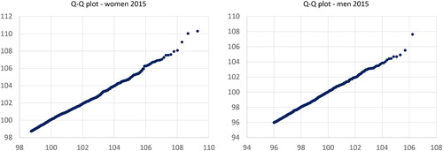
First, we consider the validity of the generalized Pareto limit in (1), necessary for setting the extreme value approach to work. We confine ourselves to the last year of death 2015: as an illustration we present, for both women (with k = 1500) and men (with k = 1000), quantile–quantile plots of the empirical quantiles above the threshold against the estimated generalized Pareto quantiles. As Figure 1 shows there is a remarkably good fit and we proceed with the extreme value analysis.

Fig. 1 Generalized Pareto Q–Q plots for women and men for the year 2015.

We first performed the formal (simultaneous) test for the null hypothesis that at least one of the 30 extreme value indices is nonnegative against the alternative hypothesis that they are all are negative, with significance level 5%. Recall that a negative extreme value index implies a finite upper endpoint of the distribution. Therefore, we first need to estimate the extreme value indices ${\gamma }_j, j=1,\dots ,30$, for the 30 years (j refers to year of death $1985+j$) and for women and for men. For these (pseudo-maximum likelihood) estimates ${\widehat{\gamma }}_j$, we will choose the sample fraction k = 1500 for women and k = 1000 for men. Recall that for the asymptotic theory it is required that $k(n)\to \infty ,k(n)/n\to 0$, as $n\to \infty$. The present values of k are indeed large, whereas the fractions $k(n)/n$ are small (n is about 70,000). We also made plots of $\widehat{\gamma }$ as a function of k for various cases and they show that for our choices there is a good balance between variance (small for large k) and squared bias (small for small k). Moreover choosing somewhat different k leads to similar results as below. The estimated extreme value indices are exhibited in Figure 2. Clearly they are all negative, hinting at a finite upper endpoint, that is, a finite maximum life span.

Fig. 2 Estimated extreme values indices for the years of death $1985+j,j=1,\dots ,30$.

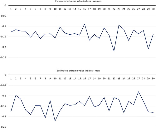
The test mentioned in the previous paragraph is, as indicated in Section 1, based on ${\widehat{\gamma }}_{\text{max}}$, the maximum of the estimated extreme value indices. The mathematical details of the test are discussed in Section 3. Here, for the women this maximum estimated index is the one corresponding to the year 2001 and it is equal to –0.089. The test leads to an asymptotic p-value of 0.0003 ($=\Phi (-0.089\sqrt{1500})$) establishing that the upper limit of the probability distribution of the human life span of Dutch women is finite for all of the 30 years under consideration. For men, the asymptotic p-value of this test is 0.0055 ($=\Phi (-0.080\sqrt{1000})$) leading to the same conclusion.

2.2 What Is the Upper Endpoint of the Life Span Distribution?

The results on the endpoints for women and men are displayed separately in Figure 3. There are four lines in each display. The blue line depicts the estimated upper endpoints ${\widehat{\omega }}_j,j=1,\dots ,30$, in years. The red line shows the 95% one-sided upper confidence bound for each year thus indicating the level of uncertainty in the estimation. The average estimated upper endpoint is 115.7 years and the maximum estimated upper endpoint, corresponding to the year 2001, is 123.7 years; the average of the upper confidence bounds is 120.3 years. In addition, the black line shows the age of the oldest person to die in each year and the gray line shows the age of the 1500th (for women) oldest person to die in each year. For men we show the 1000th oldest at death. In contrast to the estimated limits of the life span and the annual oldest women (average is 110.0), the ages of the 1500th oldest gradually increase from 95.3 to 98.7 years, an increase of about 0.11 year per calendar year. In other words, we see that the probability distribution at high age shifts toward the endpoint, over the years, but that the endpoints themselves do not increase, see the next subsection. The picture for men is similar, but the estimation results are a bit less precise than for women, since the sample fraction k is smaller. For men, the average endpoint estimate is 114.1 and the maximum endpoint estimate is 124.7; the average upper confidence bound is 119.6. The age of the 1000th oldest gradually increases from 94.5 to 96.0 years; the average oldest is 107.6.

Fig. 3 Estimated maximum human life span for the years of death $1985+j,j=1,\dots ,30$.

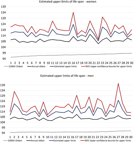
Observe that the average endpoint estimates for women and men are relatively close (1.6 years in difference only). In contrast, the average age of death during the 30 years that we consider shows a gender difference of more than 5 years.

2.3 Is There a Trend in the Maximum Human Life Span?

Visual inspection does not reveal any trend in the endpoint estimates for both genders. A “no trend” conclusion would more or less contradict the findings in Dong, Milholland, and Vijg (2016) where it is claimed that the endpoints increase at first and decrease later. That paper and its method are much contested so we performed classical linear and quadratic regression analyses to investigate this. We found no significant upward, downward, or parabolic trend, for both genders. Hence, there are no clear global changes in the maximum human lifespan over the years.

We also developed and applied an asymptotic ${\chi }^2$-test for testing the null hypothesis of equality of the upper limits of the distribution (the details are given in Section 3). For Dutch women, the asymptotic p-value is 0.0081 and hence the null hypothesis is rejected at the 5% level: the upper endpoints ${\omega }_j, j=1,\dots ,30$, are not all equal (but since this inequality of endpoints is not due to a trend, it is more of the oscillations type). For Dutch men the null hypothesis of equal endpoints is not rejected (asymptotic p-value is 0.4270), confirming that there is no trend in the endpoints.

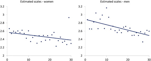
Next we consider a possible trend in the scale parameter $a_j(\frac{n}{k}),j=1,\dots ,30$. Observe that, see (2), $$\widehat{a}\left(\frac{n}{k}\right)=\left|\widehat{\gamma }\right|(\widehat{\omega }-X_{n-k,n}).$$

Since ${\widehat{\omega }}_j$ and ${\widehat{\gamma }}_j$ do not show a trend over the 30 years (see Figures 2 and 3), and since $X_{n-k,n}$ (of year j) is gradually increasing (see Figure 3), we find that the estimated scale ${\widehat{a}}_j(\frac{n}{k})$, in years, shows a clear downward trend. This is born out in Figure 4, where also a straight line is fitted to the estimated scale parameters.

Fig. 4 Estimated scale ${\widehat{a}}_j(\frac{n}{k})$ shows downward trend over the 30 years.

2.4 Force of Mortality

The force of mortality $\lambda (t):=F\prime (t)/(1-F(t))$, where t represents time, is an instantaneous measure of mortality. It is approximately (for small $\epsilon >0$) the probability of dying before time $t+\epsilon$ given survival until time t, standardized by dividing by ε. This provides a way of estimating λ. Extreme value theory offers another (here more relevant) way to estimate λ using the asymptotic relation between λ and the scale function a from Section 1 $$\underset{t\to \omega }{\lim }\lambda \left(t\right)·a\left(\frac{1}{1-F\left(t\right)}\right)=1\hspace{1em} \text{for} \text{all} \gamma \in \mathbb{R}.$$

(This relation follows for negative γ immediately from combining (1.1.37) and (1.2.14) in de Haan and Ferreira (2006).) In particular, if $k(n)\to \infty ,k(n)/n\to 0$ as $n\to \infty$, $$\begin{array}{c}\lambda \left(F^{-1}\left(1-\frac{k}{n}\right)\right)·\widehat{a}\left(\frac{n}{k}\right)\stackrel{P}{\to }1\hspace{1em}\text{and}\hspace{1em}\\ \lambda \left(X_{n-k,n}\right)·\widehat{a}\left(\frac{n}{k}\right)\stackrel{P}{\to }1\hspace{1em}\text{as} n\to \infty ,\end{array}$$ that is, the force of mortality at the time of death of the $(k+1)$st oldest, can be estimated by $1/\widehat{a}(\frac{n}{k})$ where $\widehat{a}(\frac{n}{k})$ is provided by the pseudo-maximum likelihood procedure. Note that the scale function a is regularly varying with index γ (follows from Lemma 1.2.9 in de Haan and Ferreira (2006)). Hence for s > 0 we define $\widehat{\lambda }\left(F^{-1}\left(1-\frac{\mathit{ks}}{n}\right)\right)=s^{\widehat{\gamma }}/\widehat{a}(\frac{n}{k})$. For example, when taking $s=1/k$ we obtain the “theoretical” time of death of the oldest and find $$\widehat{\lambda }\left(F^{-1}\left(1-\frac{1}{n}\right)\right)=\frac{k^{-\widehat{\gamma }}}{\widehat{a}\left(\frac{n}{k}\right)} .$$

This leads to average (over the 30 years) values of $\widehat{\lambda }((F^{-1}(1-\frac{1}{n})))$, in days, of 0.0031 for women and 0.0029 for men. Observe that when measuring time in days, the force of mortality is approximately the probability of dying the coming day.

Alternatively, we can use relation (1.1.37) of de Haan and Ferreira (2006) directly: for $\gamma <0$ $\underset{t\to \omega }{\lim }\lambda (t)(\omega -t)=-1/\gamma$, showing that the force of mortality increases quickly when approaching ω. We can estimate $\lambda (t)$ with $$\widehat{\lambda }\left(t\right)=\frac{1}{-\widehat{\gamma }(\widehat{\omega }-t)}\hspace{1em} \text{for} \text{any} \text{age} t<\widehat{\omega }.$$

When taking $t=\widehat{\omega }-1$ years, this yields an average estimated force of mortality, in days again, of 0.0206 for women and 0.0197 for men.

2.5 Perseverance Parameter

If the extreme value index is negative, the maximum life span is finite. For a person of high age t there is a maximum residual life time $\omega -t$. We are interested in the percentage of this maximum residual life time a person is living on average. The extreme value condition implies that this percentage stabilizes at high age (see Lemma A.4 in Aarssen and de Haan (1994)) $$\underset{t\to \omega }{\lim }E\left(\frac{X-t}{\omega -t} | X>t\right)=\frac{-\gamma }{1-\gamma } .$$

We call this limit α, the perseverance parameter. Using $\widehat{\alpha }=-\widehat{\gamma }/(1-\widehat{\gamma })$ we find an average $\widehat{\alpha }$ of 0.1208 for women and 0.1271 for men. Observe that α can also be seen as an approximation of the mean residual life time at the very high age of $\omega -1$ years. The just obtained average estimates lead to estimated mean residual life times at this age of about 44 and 46 days, respectively.

3 Mathematical Details of the Two Tests

3.1 Testing Whether All Extreme Value Indices Are Negative

Here we assume that the life spans for each year of death j are independent and identically distributed.

The null hypothesis to be tested is: for at least one $j=1,\dots ,30,{\gamma }_j\ge 0$ against the alternative that all ${\gamma }_j<0$; the significance level is 0.05, say. The test statistic is ${\max }_{1\le j\le 30}{\widehat{\gamma }}_j$. Assume the null hypothesis holds and ${\gamma }_{j_0}\ge 0$. From Drees, Ferreira, and de Haan (2004): if $k(n)\to \infty$ and $\sqrt{k}{A}_{j_0}(\frac{n}{k})\to 0$ as $n\to \infty$ (where $A_{j_0}$ is the second order norming function), then $\sqrt{k}({\widehat{\gamma }}_{j_0}-{\gamma }_{j_0})/(1+{\gamma }_{j_0})$ is asymptotically standard normal. Now, for $c={\Phi }^{-1}(0.05)$ $=-1.645$, (3) $$\begin{array}{c}P(\sqrt{k}\underset{{}_{1\le j\le 30}}{\max }{\widehat{\gamma }}_j\le c))=P(\underset{j=1}{\overset{30}{\cap }}\{\sqrt{k}{\widehat{\gamma }}_j\le c\})\\ \le P(\sqrt{k}{\widehat{\gamma }}_{j_0}\le c)\le P\left(\sqrt{k}\right({\widehat{\gamma }}_{j_0}-{\gamma }_{j_0})/(1+{\gamma }_{j_0})\le c),\end{array}$$(3) for $\sqrt{k}+c\ge 0$, which is the case for $k\ge 3$. The right-hand-side of (3) converges to $\Phi (-1.645)=0.05$ as $n\to \infty$. Hence, the critical region is $(-\infty ,-1.645/\sqrt{k}]$. Similarly the asymptotic p-value is equal to $\Phi (v\sqrt{k})$ where v is the value of the test statistic.

3.2 Testing Whether All Endpoints Are Equal

Here we assume, in addition, that the life spans from different years of death are also independent of each other, that is, that we have independent random samples.

In general for $\gamma <0$: if $k(n)\to \infty$ and $\sqrt{k}A(\frac{n}{k})\to 0$ (with A the second order norming function) as $n\to \infty$, then $\sqrt{k}(\widehat{\omega }-\omega )/\widehat{a}(\frac{n}{k})\stackrel{d}{\to }N(0,{\tau }^2(\gamma ))$, as $n\to \infty$, with ${\tau }^2(\gamma )=2+2{\gamma }^{-1}+5{\gamma }^{-2}+4{\gamma }^{-3}+{\gamma }^{-4}$, see pp. 146 and 147 in de Haan and Ferreira (2006). For our setup this implies $${\left(\frac{\sqrt{k}({\widehat{\omega }}_j-{\omega }_j)}{{\widehat{a}}_j\left(\frac{n}{k}\right)\tau \left({\widehat{\gamma }}_j\right)}\right)}_{j=1}^{30}\stackrel{d}{\to }{\left(Z_j\right)}_{j=1}^{30},\hspace{1em} \text{as} n\to \infty ,$$ with $Z_1,\dots ,Z_{30}$ independent standard normal random variables. Writing $d_j=k/{({\widehat{a}}_j(\frac{n}{k})\tau ({\widehat{\gamma }}_j))}^2,d={\sum }_{j=1}^{30}{d}_j$, and $r_j=d_j/d$, this can be written as (4) $${\left(\sqrt{d{r}_j}({\widehat{\omega }}_j-{\omega }_j)\right)}_{j=1}^{30}\stackrel{d}{\to }{\left(Z_j\right)}_{j=1}^{30}.$$(4)

The null hypothesis to be tested is ${\omega }_1=\cdots ={\omega }_{30}$, against the alternative that the ω_j are not all equal. We use the test statistic $$T=d·\sum _{j=1}^{30}{r}_j{({\widehat{\omega }}_j-\tilde{\omega })}^2,$$ with $\tilde{\omega }={\sum }_{j=1}^{30}{r}_j{\widehat{\omega }}_j$. Now assume $r_j\stackrel{P}{\to }{\rho }_j$, for certain constants ${\rho }_j,j=1,\dots ,30$. Under H₀, we have $T=d{\sum }_{j=1}^{30}{r}_j{({\widehat{\omega }}_j-\omega )}^2-d{(\tilde{\omega }-\omega )}^2$, with ω the common value of the ω_j. Then by (4) the limit in distribution of T is ${\sum }_{j=1}^{30}{Z}_j^2-{\left({\sum }_{j=1}^{30}\sqrt{{\rho }_j}{Z}_j\right)}^2.$ Since ${\sum }_{j=1}^{30}{\rho }_j={\sum }_{j=1}^{30}{r}_j=1$, that is, $(\sqrt{{\rho }_1},\dots ,\sqrt{{\rho }_{30}})$ is a unit vector, this limiting random variable is well-known to have a ${\chi }_{29}^2$-distribution. [In fact the condition $r_j\stackrel{P}{\to }{\rho }_j$ can be weakened to $r_j-{\rho }_{j,n}\stackrel{P}{\to }0$ for deterministic sequences ${\rho }_{j,n}$.]

Acknowledgments

We are grateful to Fanny Janssen (University of Groningen) for crucial help with obtaining the data and for several fruitful discussions.

Additional information

Funding

The research of Laurens de Haan has been funded by FCT—Fundação para a Ciência e a Tecnologia, Portugal, through the project UID/MAT/00006/2013.

References

- Aarssen, K., and de Haan, L. (1994), “On the Maximal Life Span of Humans,” Mathematical Population Studies, 4, 259–281. DOI: 10.1080/08898489409525379.
- de Haan, L., and Ferreira, A. (2006), Extreme Value Theory: An Introduction, New York: Springer.
- Dong, X., Milholland, B., and Vijg, J. (2016), “Evidence for a Limit to Human Life Span,” Nature, 538, 257–259. DOI: 10.1038/nature19793.
- Drees, H., Ferreira, A., and de Haan, L. (2004), “On Maximum Likelihood Estimation of the Extreme Value Index,” Annals of Applied Probability, 14, 1179–1201. DOI: 10.1214/105051604000000279.
- Gampe, J. (2010), “Human Mortality Beyond Age 110,” in Supercentenarians, Demographic Research Monographs (Vol. 7), Berlin, Heidelberg: Springer, pp. 219–230.
- Gbari, S., Poulain, M., Dal, L., and Denuit, M. (2017), “Extreme Value Analysis of Mortality at the Oldest Ages: A Case Study Based on Individual Ages at Death,” North American Actuarial Journal, 21, 397–416. DOI: 10.1080/10920277.2017.1301260.
- Hanayama, N., and Sibuya, M. (2016), “Estimating the Upper Limit of Lifetime Probability Distribution, Based on Data of Japanese Centenarians,” Journals of Gerontology, Series A, 71, 1014–1021. DOI: 10.1093/gerona/glv113.
- Rootzén, H., and Zholud, D. (2017), “Human Life Is Unlimited—But Short,” Extremes, 20, 713–728. DOI: 10.1007/s10687-017-0305-5.
- Watts, K., Dupuis, D., and Jones, B. (2006), “An Extreme Value Analysis of Advanced Age Mortality Data,” North American Actuarial Journal, 10, 162–178. DOI: 10.1080/10920277.2006.10597419.
- Weon, B., and Je, J. (2009), “Theoretical Estimation of Maximum Human Lifespan,” Biogerontology, 10, 65–71. DOI: 10.1007/s10522-008-9156-4.