On the Length of Post-Model-Selection Confidence Intervals Conditional on Polyhedral Constraints

Abstract

Valid inference after model selection is currently a very active area of research. The polyhedral method, introduced in an article by Lee et al., allows for valid inference after model selection if the model selection event can be described by polyhedral constraints. In that reference, the method is exemplified by constructing two valid confidence intervals when the Lasso estimator is used to select a model. We here study the length of these intervals. For one of these confidence intervals, which is easier to compute, we find that its expected length is always infinite. For the other of these confidence intervals, whose computation is more demanding, we give a necessary and sufficient condition for its expected length to be infinite. In simulations, we find that this sufficient condition is typically satisfied, unless the selected model includes almost all or almost none of the available regressors. For the distribution of confidence interval length, we find that the κ-quantiles behave like $1/(1-\kappa )$ for κ close to 1. Our results can also be used to analyze other confidence intervals that are based on the polyhedral method.

KEYWORDS:

• Confidence interval
• Hypothesis test
• Inference after model selection
• Lasso

1 Introduction

Lee et al. (2016) recently introduced a new technique for valid inference after model selection, the so-called polyhedral method. Using this method, and using the Lasso for model selection in linear regression, Lee et al. (2016) derived two new confidence sets that are valid conditional on the outcome of the model selection step. More precisely, let $\widehat{m}$ denote the model containing those regressors that correspond to nonzero coefficients of the Lasso estimator, and let $\widehat{s}$ denote the sign-vector of those nonzero Lasso coefficients. Then Lee et al. (2016) constructed confidence intervals $[L_{\widehat{m},\widehat{s}},U_{\widehat{m},\widehat{s}}]$ and $[L_{\widehat{m}},U_{\widehat{m}}]$ whose coverage probability is $1-\alpha$, conditional on the events $\{\widehat{m}=m,\widehat{s}=s\}$ and $\{\widehat{m}=m\}$, respectively (provided that the probability of the conditioning event is positive). The computational effort in constructing these intervals is considerably lighter for $[L_{\widehat{m},\widehat{s}},U_{\widehat{m},\widehat{s}}]$. In simulations, Lee et al. (2016) noted that this latter interval can be quite long in some cases; cf. Figure 10 in that reference. We here analyze the lengths of these intervals through their (conditional) means and through their quantiles.

We focus here on the original proposal of Lee et al. (2016) for the sake of simplicity and ease of exposition. Nevertheless, our findings also carry over to several recent developments that rely on the polyhedral method and that are mentioned in Section 1.2; see Remark 1(i) and Remark 3.

1.1 Overview of Findings

Throughout, we use the same setting and assumptions as Lee et al. (2016). In particular, we assume that the response vector is distributed as $N(\mu ,{\sigma }^2{I}_n)$ with unknown mean $\mu \in {\mathbb{R}}^n$ and known variance ${\sigma }^2>0$ (our results carry over to the unknown-variance case; see Section 3.3), and that the nonstochastic regressor matrix has columns in general position. Write ${\mathbb{P}}_{\mu ,{\sigma }^2}$ and ${\mathbb{E}}_{\mu ,{\sigma }^2}$ for the probability measure and the expectation operator, respectively, corresponding to $N(\mu ,{\sigma }^2{I}_n)$.

For the interval $[L_{\widehat{m},\widehat{s}},U_{\widehat{m},\widehat{s}}]$, we find the following: Fix a nonempty model m, a sign-vector s, as well as $\mu \in {\mathbb{R}}^n$ and ${\sigma }^2>0$. If ${\mathbb{P}}_{\mu ,{\sigma }^2}(\widehat{m}=m,\widehat{s}=s)>0$, then(1) $${\mathbb{E}}_{\mu ,{\sigma }^2}\left[U_{\widehat{m},\widehat{s}}-L_{\widehat{m},\widehat{s}}|\widehat{m}=m,\widehat{s}=s\right]=\infty ;$$(1) see Proposition 2 and the attending discussion. Obviously, this statement continues to hold if the event $\widehat{m}=m,\widehat{s}=s$ is replaced by the larger event $\widehat{m}=m$ throughout. And this statement continues to hold if the condition ${\mathbb{P}}_{\mu ,{\sigma }^2}(\widehat{m}=m,\widehat{s}=s)>0$ is dropped and the conditional expectation in (1) is replaced by the unconditional one.

For the interval $[L_{\widehat{m}},U_{\widehat{m}}]$, we derive a necessary and sufficient condition for its expected length to be infinite, conditional on the event $\widehat{m}=m$; cf. Proposition 3. That condition is never satisfied if the model m is empty or includes only one regressor; it is also typically never satisfied if m includes all available regressors (see Corollary 1). The necessary and sufficient condition depends on the regressor matrix, on the model m and also on a linear contrast that defines the quantity of interest, and is daunting to verify in all but the most basic examples. We also provide a sufficient condition for infinite expected length that is easy to verify. In simulations, we find that this sufficient condition for infinite expected length is typically satisfied except for two somewhat extreme cases: (a) If the Lasso penalty is very large (so that almost all regressors are excluded). (b) If the number of available regressors is not larger than sample size and the Lasso parameter is very small (so that almost no regressor is excluded). See Figure 3 for more detail.

Of course, a confidence interval with infinite expected length can still be quite short with high probability. In our theoretical analysis and in our simulations, we find that the κ-quantiles of $U_{\widehat{m},\widehat{s}}-L_{\widehat{m},\widehat{s}}$ and $U_{\widehat{m}}-L_{\widehat{m}}$ behave like the κ-quantiles of $1/U$ with $U\sim U(0,1)$, that is, like $1/(1-\kappa )$, for κ close to 1 if the conditional expected length of these intervals is infinite; cf. Proposition 4, Figure 4 and the attending discussions.

The methods developed in this article can also be used if the Lasso, as the model selector, is replaced by any other procedure that relies on the polyhedral method; see Remark 1(i) and Remark 3. In particular, we see that confidence intervals based on the polyhedral method in Gaussian regression can have infinite expected length. Our findings suggest that the expected length of confidence intervals based on the polyhedral method should be closely scrutinized, in Gaussian regression but also in non-Gaussian settings and other variations of the polyhedral method.

“Length” is arguably only one of several possible criteria for judging the “quality” of valid confidence intervals, albeit one of practical interest. Our focus on confidence interval length is justified by our findings.

The rest of the article is organized as follows: We conclude this section by discussing a number of related results that put our findings in context. Section 2 describes the confidence intervals of Lee et al. (2016) in detail and introduces some notation. Section 3 contains our core results, Propositions 1–4 which entail our main findings, as well as a discussion of the unknown variance case. The simulation studies mentioned earlier are given in Section 4. Finally, in Section 5, we discuss some implications of our findings. In particular, we argue that the computational simplicity of the polyhedral method comes at a price in terms of interval length, and that computationally more involved methods can provide a remedy. The appendix contains the proofs and some auxiliary lemmas.

1.2 Context and Related Results

There are currently several exciting ongoing developments based on the polyhedral method, not least because it proved to be applicable to more complicated settings, and there are several generalizations of this framework (see, among others, Fithian et al. 2015; Gross, Taylor, and Tibshirani 2015; Reid, Taylor, and Tibshirani 2015; Tian and Taylor 2016, 2017; Tian et al. 2016; Tibshirani et al. 2016; Tian, Loftus, and Taylor 2017; Markovic, Xia, and Taylor 2018; Panigrahi, Zhu, and Sabatti 2018; Taylor and Tibshirani 2018; Panigrahi and Taylor 2019). Certain optimality results of the method of Lee et al. (2016) are given in Fithian, Sun, and Taylor (2017). Using a different approach, Berk et al. (2013) proposed the so-called PoSI-intervals which are unconditionally valid. A benefit of the PoSI-intervals is that they are valid after selection with any possible model selector, instead of a particular one like the Lasso; however, as a consequence, the PoSI-intervals are typically very conservative (i.e., the actual coverage probability is above the nominal level). Nonetheless, Bachoc, Leeb, and Pötscher (2019) showed in a Monte Carlo simulation that, in certain scenarios, the PoSI-intervals can be shorter than the intervals of Lee et al. (2016). The results of the present article are based on the first author’s master’s thesis.

It is important to note that all confidence sets discussed so far are nonstandard, in the sense that the parameter to be covered is not the true parameter in an underlying correct model (or components thereof), but instead is a model-dependent quantity of interest. (See Section 2 for details and the references in the preceding paragraph for more extensive discussions.) An advantage of this nonstandard approach is that it does not rely on the assumption that any of the candidate models is correct. Valid inference for an underlying true parameter is a more challenging task, as demonstrated by the impossibility results in Leeb and Pötscher (2006a, 2006b, 2008). There are several proposals of valid confidence intervals after model selection (in the sense that the actual coverage probability of the true parameter is at or above the nominal level) but these are rather large compared to the standard confidence intervals from the full model (supposing that one can fit the full model); see Pötscher (2009), Pötscher and Schneider (2010), and Schneider (2016). In fact, Leeb and Kabaila (2017) showed that the usual confidence interval obtained by fitting the full model is admissible also in the unknown variance case; therefore, one cannot obtain uniformly smaller valid confidence sets for a component of the true parameter by any other method.

2 Assumptions and Confidence Intervals

Let Y denote the $N(\mu ,{\sigma }^2{I}_n)$-distributed response vector, $n\ge 1$, where $\mu \in {\mathbb{R}}^n$ is unknown and ${\sigma }^2>0$ is known. Let $X=(x_1,\dots ,x_p),p\ge 1$, with $x_i\in {\mathbb{R}}^n$ for each $i=1,\dots ,p$, be the nonstochastic n × p regressor matrix. We assume that the columns of X are in general position (this mild assumption is further discussed in the following paragraph). The full model $\{1,\dots ,p\}$ is denoted by m_F. All subsets of the full model are collected in $\mathcal{M}$, that is, $\mathcal{M}=\{m:m\subseteq m_F\}$. The cardinality of a model m is denoted by $\left|m\right|$. For any $m=\{i_1,\dots ,i_k\}\in \mathcal{M}\setminus \varnothing$ with $i_1<\dots <i_k$, we set $X_m=(x_{i_1},\dots ,x_{i_k})$. Analogously, for any vector $v\in {\mathbb{R}}^p$, we set $v_m=(v_{i_1},\dots ,v_{i_k})\prime$. If m is the empty model, then X_m is to be interpreted as the zero vector in ${\mathbb{R}}^n$ and v_m as 0.

The Lasso estimator, denoted by $\widehat{\beta }(y)$, is a minimizer of the least squares problem with an additional penalty on the absolute size of the regression coefficients (Frank and Friedman 1993; Tibshirani 1996):$$\underset{\beta \in {\mathbb{R}}^p}{\text{min}}\frac{1}{2}⏧y-X\beta {⏧}_2^2+\lambda ⏧\beta {⏧}_1,\hspace{1em}y\in {\mathbb{R}}^n,\lambda >0.$$

The Lasso has the property that some coefficients of $\widehat{\beta }(y)$ are zero with positive probability. A minimizer of the Lasso objective function always exists, but it is not necessarily unique. Uniqueness of $\widehat{\beta }(y)$ is guaranteed here by our assumption that the columns of X are in general position (Tibshirani 2013). This assumption is relatively mild; for example, if the entries of X are drawn from a (joint) distribution that has a Lebesgue density, then the columns of X are in general position with probability 1 (Tibshirani 2013). The model $\widehat{m}(y)$ selected by the Lasso and the sign-vector $\widehat{s}(y)$ of nonzero Lasso coefficients can now formally be defined through$$\widehat{m}(y)=\left\{j:{\widehat{\beta }}_j(y)\ne 0\right\}\hspace{1em}\text{and}\hspace{1em}\widehat{s}(y)=\text{sign}\left({\widehat{\beta }}_{\widehat{m}(y)}(y)\right),$$

(where $\widehat{s}(y)$ is left undefined if $\widehat{m}(y)=\varnothing$). Recall that $\mathcal{M}$ denotes the set of all possible submodels and set ${\mathcal{S}}_m={\{-1,1\}}^{\left|m\right|}$ for each $m\in \mathcal{M}$. For later use we also denote by ${\mathcal{M}}^{+}$ and ${\mathcal{S}}_m^{+}$ the collection of models and the collection of corresponding sign-vectors, that occur with positive probability, that is,$$\begin{array}{c}{\mathcal{M}}^{+}=\left\{m\in \mathcal{M}:{\mathbb{P}}_{\mu ,{\sigma }^2}(\widehat{m}(Y)=m)>0\right\},\\ \mathrm{}\mathrm{}{\mathcal{S}}_m^{+}=\{s\in {\mathcal{S}}_m:{\mathbb{P}}_{\mu ,{\sigma }^2}(\widehat{m}(Y)=m,\widehat{s}(Y)=s)>0\}\mathrm{\hspace{1em}}\mathrm{\hspace{1em}}(m\in \mathcal{M}).\end{array}$$

These sets do not depend on μ and ${\sigma }^2$ as the measure ${\mathbb{P}}_{\mu ,{\sigma }^2}$ is equivalent to Lebesgue measure with respect to null sets. Also, our assumption that the columns of X are in general position guarantees that ${\mathcal{M}}^{+}$ only contains models m for which X_m has column-rank m (Tibshirani 2013).

Inference is focused on a nonstandard, model dependent, quantity of interest. Consider first the nontrivial case where $m\in {\mathcal{M}}^{+}\setminus \{\varnothing \}$. In that case, we set$${\beta }^m={\mathbb{E}}_{\mu ,{\sigma }^2}\left[{(X_m^{\prime }{X}_m)}^{-1}{X}_m^{\prime }Y\right]={(X_m^{\prime }{X}_m)}^{-1}{X}_m^{\prime }\mu .$$

For ${\gamma }^m\in {\mathbb{R}}^{\left|m\right|}\setminus \left\{0\right\}$, the goal is to construct a confidence interval for ${\gamma }^{m\prime }{\beta }^m$ with conditional coverage probability $1-\alpha$ on the event $\{\widehat{m}=m\}$. Clearly, the quantity of interest can also be written as ${\gamma }^{m\prime }{\beta }^m={\eta }^{m\prime }\mu$ for ${\eta }^m=X_m{(X_m^{\prime }{X}_m)}^{-1}{\gamma }^m$. For later use, write $P_{{\eta }^m}$ for the orthogonal projection on the space spanned by η^m. Finally, for the trivial case where $m=\varnothing$, we set ${\beta }^{\varnothing }={\gamma }^{\varnothing }={\eta }^{\varnothing }=0$.

At the core of the polyhedral method lies the observation that the event where $\widehat{m}=m$ and where $\widehat{s}=s$ describes a convex polytope in sample space ${\mathbb{R}}^n$ (up to a Lebesgue null set): Fix $m\in {\mathcal{M}}^{+}\setminus \{\varnothing \}$ and $s\in {\mathcal{S}}_m^{+}$. Then(2) $$\left\{y:\widehat{m}(y)=m,\widehat{s}(y)=s\right\}\hspace{1em}\stackrel{\mathrm{a}.\mathrm{s}.}{=}\hspace{1em}\{y:A_{m,s}y<b_{m,s}\};$$(2) see Theorem 3.3 in Lee et al. (2016) (explicit formulas for the matrix $A_{m,s}$ and the vector $b_{m,s}$ are also repeated in Appendix C in our notation). Fix $z\in {\mathbb{R}}^n$ orthogonal to η^m. Then the set of y satisfying $(I_n-P_{{\eta }^m})y=z$ and $A_{m,s}y<b$ is either empty or a line segment. In either case, that set can be written as $\{z+{\eta }^{m}w:{\mathcal{V}}_{m,s}^{-}(z)<w<{\mathcal{V}}_{m,s}^{+}(z)\}$. The endpoints satisfy $-\infty \le {\mathcal{V}}_{m,s}^{-}(z)\le {\mathcal{V}}_{m,s}^{+}(z)\le \infty$ [see Lemma 4.1 of Lee et al. (2016); formulas for these quantities are also given in Appendix C in our notation]. Now decompose Y into the sum of two independent Gaussians $P_{{\eta }^m}Y$ and $(I_n-P_{{\eta }^m})Y$, where the first one is a linear function of ${\eta }^{m\prime }Y\sim N({\eta }^{m\prime }\mu ,{\sigma }^2{\eta }^{m\prime }{\eta }^m)$. With this, the conditional distribution of ${\eta }^{m\prime }Y$, conditional on the event $\{\widehat{m}(Y)=m,\widehat{s}(Y)=s,(I_n-P_{{\eta }^m})=z\}$, is the conditional $N({\eta }^{m\prime }\mu ,{\sigma }^2{\eta }^{m\prime }{\eta }^m)$-distribution, conditional on the set $({\mathcal{V}}_{m,s}^{-}(z),{\mathcal{V}}_{m,s}^{+}(z))$ (in the sense that the latter conditional distribution is a regular conditional distribution if one starts with the conditional distribution of ${\eta }^{m\prime }Y$ given $\widehat{m}=m$ and $\widehat{s}=s$—which is always well-defined—and if one then conditions on the random variable $(I_n-P_{{\eta }^m})Y$).

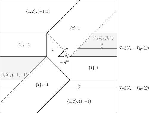
Fig. D1 For n = 2, the sample space ${\mathbb{R}}^2$ is partitioned corresponding to the model and the sign-vector selected by the Lasso when λ = 2 and $X=(x_1:x_2)$, with $x_1=(1,0)\prime$ and $x_2=(1,1)\prime$. We set $m=\{1,2\}$ and ${\gamma }^m=(1,1)$, so that ${\eta }^m=x_1$. The point y lies on the black line segment $\{z+{\eta }^{m}v:v\in T_m(z)\}$ for $z=(I_2-P_{\eta })y$, which is bounded on the left. In particular, $T_m(z)$ is bounded. For the point $\tilde{y}$, the corresponding black line segments together are unbounded on both sides, and hence $T_m((I_2-P_{{\eta }_m})\tilde{y})$ is unbounded.

To use these observations for the construction of confidence sets, consider first the conditional distribution of a random variable $V\sim N(\theta ,{\varsigma }^2)$ conditional on the event $V\in T$, where $\theta \in \mathbb{R}$, where ${\varsigma }^2>0$ and where $T\ne \varnothing$ is the union of finitely many open intervals. The intervals may be unbounded. Write $F_{\theta ,{\varsigma }^2}^T(·)$ for the cumulative distribution function (cdf) of V given $V\in T$. The corresponding law can be viewed as a “truncated normal” distribution and will be denoted by $TN(\theta ,{\varsigma }^2,T)$ in the following. We will construct a confidence interval based on W, where $W\sim TN(\theta ,{\varsigma }^2,T)$. Such an interval, which covers θ with probability $1-\alpha$, is obtained by the usual method of collecting all values θ₀ for which a hypothesis test of $H_0:\theta ={\theta }_0$ against $H_1:\theta \ne {\theta }_0$ does not reject, based on the observation $W\sim TN(\theta ,{\varsigma }^2,T)$. In particular, for $w\in \mathbb{R}$, define L(w) and U(w) through$$F_{L(w),{\varsigma }^2}^T(w)=1-\frac{\alpha }{2}\hspace{1em}\text{and}\hspace{1em}{F}_{U(w),{\varsigma }^2}^T(w)=\frac{\alpha }{2},$$which are well-defined in view of Lemma A.2. With this, we have $P(\theta \in [L(W),U(W)])=1-\alpha$ irrespective of $\theta \in \mathbb{R}$.

Fix $m\in {\mathcal{M}}^{+}\setminus \{\varnothing \}$ and $s\in {\mathcal{S}}_m^{+}$, and let ${\sigma }_m^2={\sigma }^2{\eta }^{m\prime }{\eta }^m$ and $T_{m,s}(z)=({\mathcal{V}}_{m,s}^{-}(z),{\mathcal{V}}_{m,s}^{+}(z))$ for z orthogonal to η^m. With this, we have(3) $${\eta }^{m\prime }Y\left|\right\{\widehat{m}=m,\widehat{s}=s,(I_n-P_{{\eta }^m})Y=z\}\sim TN({\eta }^{m\prime }\mu ,{\sigma }_m^2,T_{m,s}(z))$$(3) for each $z\in \{(I_n-P_{{\eta }^m})y:A_{m,s}y<b_{m,s}\}$. Now define $L_{m,s}(y)$ and $U_{m,s}(y)$ through$$F_{L_{m,s}(y),{\sigma }_m^2}^{T_{m,s}((I_n-P_{{\eta }^m})y)}({\eta }^{m\prime }y)=1-\frac{\alpha }{2}\hspace{1em}\text{and}\hspace{1em}{F}_{U_{m,s}(y),{\sigma }_m^2}^{T_{m,s}((I_n-P_{{\eta }^m})y)}({\eta }^{m\prime }y)=\frac{\alpha }{2}$$

for each y so that $A_{m,s}y<b_{m,s}$. By the considerations in the preceding paragraph, it follows that(4) $${\mathbb{P}}_{\mu ,{\sigma }^2}({\eta }^{m\prime }\mu \in [L_{m,s}(Y),U_{m,s}(Y)\left]\right|\widehat{m}=m,\widehat{s}=s,(I_n-P_{{\eta }^m})Y=z)=1-\alpha .$$(4)

Clearly, the random interval $[L_{m,s}(Y),U_{m,s}(Y)]$ covers ${\gamma }^{m\prime }{\beta }^m={\eta }^{m\prime }\mu$ with probability $1-\alpha$ also conditional on the event that $\widehat{m}=m$ and $\widehat{s}=s$ or on the event that $\widehat{m}=m$.

In a similar fashion, fix $m\in {\mathcal{M}}^{+}$. In the nontrivial case where $m\ne \varnothing$, we set $T_m(z)={\cup }_{s\in {\mathcal{S}}_m^{+}}{T}_{m,s}(z)$ for z orthogonal to η^m, and define $L_m(y)$ and $U_m(y)$ through$$F_{L_m(y),{\sigma }_m^2}^{T_m((I_n-P_{{\eta }^m})y)}({\eta }^{m\prime }y)=1-\frac{\alpha }{2}\hspace{1em}\text{and}\hspace{1em}{F}_{U_m(y),{\sigma }_m^2}^{T_m((I_n-P_{{\eta }^m})y)}({\eta }^{m\prime }y)=\frac{\alpha }{2}.$$

Arguing as in the preceding paragraph, we see that the random interval $[L_m(Y),U_m(Y)]$ covers ${\gamma }^{m\prime }{\beta }^m={\eta }^{m\prime }\mu$ with probability $1-\alpha$ conditional on any of the events $\{\widehat{m}=m,(I_n-P_{{\eta }^m})Y=z\}$ and $\{\widehat{m}=m\}$. In the trivial case where $m=\varnothing$, we set $[L_{\varnothing }(Y),R_{\varnothing }(Y)]=\left\{0\right\}$ with probability $1-\alpha$ and $[L_{\varnothing }(Y),R_{\varnothing }(Y)]=\left\{1\right\}$ with probability α, so that similar coverage properties also hold in that case. The unconditional coverage probability of the interval $[L_{\widehat{m}}(Y),R_{\widehat{m}}(Y)]$ then also equals $1-\alpha$.

Remark 1.

1. If $\tilde{m}=\tilde{m}(y)$ is any other model selection procedure, so that the event $\{\tilde{m}=m\}$ can be represented as the union of a finite number of polyhedra (up to null sets), then the polyhedral method can be applied to obtain a confidence set for ${\eta }^{m\prime }\mu$ with conditional coverage probability $1-\alpha$, conditional on the event $\{\tilde{m}=m\}$, if that event has positive probability.

2. We focus here on equal-tailed confidence intervals for the sake of brevity. It is easy to adapt all our results to the unequal-tailed case, that is, the case where $\alpha /2$ and $1-\alpha /2$ are replaced by α₁ and $1-{\alpha }_2$ with only minor modifications of the proofs, provided that α₁ and α₂ are are both in (0,1/2]. (The remaining case, in which $1/2<{\alpha }_1+{\alpha }_2<1$, is of little interest, because the corresponding coverage probability is $1-{\alpha }_1-{\alpha }_2<1/2$ here, and is left as an exercise.) Another alternative, the uniformly most accurate unbiased interval, is discussed at the end of Section 5.

3. In Theorem 3.3 of Lee et al. (2016), relation (2) is stated as an equality, not as an equality up to null sets, and with the right-hand side replaced by $\{y:A_{m,s}y\le b_{m,s}\}$ (in our notation). Because (2) differs from this only on a Lebesgue null set, the difference is inconsequential for the purpose of the present article. The statement in Lee et al. (2016) is based on the fact that $\widehat{m}$ was defined as the equicorrelation set (Tibshirani 2013) in that article. But if $\widehat{m}$ is the equicorrelation set, then there can exist vectors $y\in \{\widehat{m}=m\}$ such that some coefficients of $\widehat{\beta }(y)$ are zero, which clashes with the idea that $\widehat{m}$ contains those variables whose Lasso coefficients are nonzero. However, for any $m\in {\mathcal{M}}^{+}$, the set of such y’s is a Lebesgue null set.

3 Analytical Results

3.1 Mean Confidence Interval Length

We first analyze the simple confidence set $[L(W),U(W)]$ introduced in the preceding section, which covers θ with probability $1-\alpha$, where $W\sim TN(\theta ,{\varsigma }^2,T)$. By assumption, T is of the form $T={\cup }_{i=1}^K(a_i,b_i)$ where $K<\infty$ and $-\infty \le a_1<b_1<\cdots <a_K<b_K\le \infty$. Figure 1 exemplifies the length of $[L(w),U(w)]$ when T is bounded (left panel) and when T is unbounded (right panel). The dashed line corresponds to the length of the standard (unconditional) confidence interval for θ based on $V\sim N(\theta ,{\varsigma }^2)$. In the left panel, we see that the length of $[L(w),U(w)]$ diverges as w approaches the far left or the far right boundary point of the truncation set (i.e., –3 and 3). On the other hand, in the right panel we see that the length of $[L(w),U(w)]$ is bounded and converges to the length of the standard interval as $\left|w\right|\to \infty$.

Fig. 1 Length of the interval $[L(w),U(w)]$ for the case where $T=(-3,-2)\cup (-1,1)\cup (2,3)$ (left panel) and the case where $T=(-\infty ,-2)\cup (-1,1)\cup (2,\infty )$ (right panel). In both cases, we took ${\varsigma }^2=1$ and $\alpha =0.05$.

Write $\Phi (w)$ and $\varphi (w)$ for the cdf and pdf of the standard normal distribution, respectively, where we adopt the usual convention that $\Phi (-\infty )=0$ and $\Phi (\infty )=1$.

Proposition 1

(The interval $[L(W),U(W)]$ for truncated normal W). Let $W\sim TN(\theta ,{\varsigma }^2,T)$. If T is bounded either from above or from below, then$$E[U(W)-L(W)]=\infty .$$

If T is unbounded from above and from below, then$$\begin{array}{c}\frac{U(W)-L(W)}{\varsigma }\stackrel{\mathrm{a}.\mathrm{s}.}{\le }2{\Phi }^{-1}(1-p_{\ast }\alpha /2)\\ \stackrel{}{\le }2{\Phi }^{-1}(1-\alpha /2)+\frac{a_K-b_1}{\varsigma },\end{array}$$where $p_{\ast }=\underset{\vartheta \in \mathbb{R}}{\inf }P(N(\vartheta ,{\varsigma }^2)\in T)$ and where $a_K-b_1$ is to be interpreted as 0 in case K = 1. [The first inequality trivially continues to hold if T is bounded, as then $p_{\ast }=0$.]

Intuitively, one expects confidence intervals to be wide if one conditions on a bounded set because extreme values cannot be observed on a bounded set and the confidence intervals have to take this into account. We find that the conditional expected length is infinite in this case. If, for example, T is bounded from below, that is, if $-\infty <a_1$, then the first statement in the proposition follows from two facts: First, the length of $U(w)-L(w)$ behaves like $1/(w-a_1)$ as w approaches a₁ from above; and, second, the pdf of the truncated normal distribution at w is bounded away from 0 as w approaches a₁ from above. See the proof in Section B for a more detailed version of this argument. On the other hand, if the truncation set is unbounded, extreme values are observable and confidence intervals, therefore, do not have to be extremely wide. The second upper bound provided by the proposition for that case will be useful later.

We see that the boundedness of the truncation set T is critical for the interval length. When the Lasso is used as a model selector, this prompts the question whether the truncation sets $T_{m,s}(z)$ and $T_m(z)$ are bounded or not, because the intervals $[L_{m,s}(y),U_{m,s}(y)]$ and $[L_m(y),U_m(y)]$ are obtained from conditional normal distributions with truncation sets $T_{m,s}((I_n-P_{{\eta }^m})y)$ and $T_m((I_n-P_{{\eta }^m})y)$, respectively. For $m\in {\mathcal{M}}^{+}\setminus \{\varnothing \},s\in {\mathcal{S}}_m^{+}$, and z orthogonal to η^m, recall that $T_{m,s}(z)=({\mathcal{V}}_{m,s}^{-}(z),{\mathcal{V}}_{m,s}^{+}(z))$, and that $T_m(z)$ is the union of these intervals over $s\in {\mathcal{S}}_m^{+}$. Write ${[{\eta }^m]}^{\perp }$ for the orthogonal complement of the span of η^m.

Proposition 2

(The interval $[L_{\widehat{m},\widehat{s}}(Y),U_{\widehat{m},\widehat{s}}(Y)]$ for the Lasso). For each $m\in {\mathcal{M}}^{+}\setminus \{\varnothing \}$ and each $s\in {\mathcal{S}}_m$, we have$$\forall z\in {\left[{\eta }^m\right]}^{\perp }:-\infty <{\mathcal{V}}_{m,s}^{-}(z)\hspace{1em}\text{or}\hspace{1em}\forall z\in {\left[{\eta }^m\right]}^{\perp }:{\mathcal{V}}_{m,s}^{+}(z)<\infty$$or both.

For the confidence interval $[L_{\widehat{m},\widehat{s}}(Y),U_{\widehat{m},\widehat{s}}(Y)]$, the statement in (1) now follows immediately: If m is a nonempty model and s is a sign-vector so that the event $\{\widehat{m}=m,\widehat{s}=s\}$ has positive probability, then $m\in {\mathcal{M}}^{+}\setminus \{\varnothing \}$ and $s\in {\mathcal{S}}_m^{+}$. Now Proposition 2 entails that $T_{m,s}((I_n-P_{{\eta }^m})Y)$ is almost surely bounded on the event $\{\widehat{m}=m,\widehat{s}=s\}$, and Proposition 1 entails that (1) holds.

For the confidence interval $[L_{\widehat{m}}(Y),U_{\widehat{m}}(Y)]$, we obtain that its conditional expected length is finite, conditional on $\widehat{m}=m$ with $m\in {\mathcal{M}}^{+}\setminus \{\varnothing \}$, if and only if its corresponding truncation set $T_m(Y)$ is almost surely unbounded from above and from below on that event. More precisely, we have the following result.

Proposition 3

(The interval $[L_{\widehat{m}}(Y),U_{\widehat{m}}(Y)]$ for the Lasso). For $m\in {\mathcal{M}}^{+}\setminus \{\varnothing \}$, we have(5) $${\mathbb{E}}_{\mu ,{\sigma }^2}[U_{\widehat{m}}(Y)-L_{\widehat{m}}(Y)|\widehat{m}=m]=\infty$$(5)

if and only if there exists a $s\in {\mathcal{S}}_m^{+}$ and a vector y satisfying $A_{m,s}y<b_{m,s}$, so that(6) $$T_m((I_n-P_{{\eta }^m})y)\mathrm{}\text{is}\mathrm{}\text{bounded}\mathrm{}\text{from}\mathrm{}\text{above}\mathrm{}\text{or}\mathrm{}\text{from}\mathrm{}\text{below}.$$(6)

To infer (5) from (6), that latter condition needs to be checked for every point y in a union of polyhedra. While this is easy in some simple examples like, say, the situation depicted in Figure 1 of Lee et al. (2016), searching over polyhedra in ${\mathbb{R}}^n$ is hard in general. In practice, one can use a simpler sufficient condition that implies (5): After observing the data, that is, after observing a particular value $y^{\ast }$ of Y, and hence also observing $\widehat{m}(y^{\ast })=m$ and $\widehat{s}(y^{\ast })=s$, we check whether $T_m((I_n-P_{{\eta }^m})y^{\ast })$ is bounded from above or from below (and also whether $m\ne \varnothing$ and whether $A_{m,s}{y}^{\ast }<b_{m,s}$, which, if satisfied, entails that $m\in {\mathcal{M}}^{+}$ and that $s\in {\mathcal{S}}_m^{+}$). If this is the case, then it follows, ex post, that (5) holds. Note that these computations occur naturally during the computation of $[L_m(y^{\ast }),U_m(y^{\ast })]$ and can hence be performed as a safety precaution with little extra effort.

The next result shows that the expected length of $[L_{\widehat{m}}(Y),U_{\widehat{m}}(Y)]$ is typically finite conditional on $\widehat{m}=m$ if the selected model m is either extremely large or extremely small.

Corollary 1

(The interval $[L_{\widehat{m}}(Y),U_{\widehat{m}}(Y)]$ for the Lasso). If $\left|m\right|=0$ or $\left|m\right|=1$, we always have $E_{\mu ,{\sigma }^2}[U_{\widehat{m}}(Y)-L_{\widehat{m}}(Y)|\widehat{m}=m]<\infty$; the same is true if $\left|m\right|=p$ for Lebesgue-almost all γ^m (recall that $[L_{\widehat{m}}(Y),U_{\widehat{m}}(Y)]$ is meant to cover ${\gamma }^{m\prime }{\beta }^m$ conditional on $\widehat{m}=m$).

The corollary raises the suspicion that the conditional expected length of $[L_{\widehat{m}}(Y),U_{\widehat{m}}(Y)]$ could also be finite if the selected model m either includes almost no regressor ($\left|m\right|$ close to zero) or excludes almost no regressor ($\left|m\right|$ close to p). Our simulations seem to support this; see Figure 3. The statement concerning Lebesgue-almost all γ^m does not necessarily hold for all γ^m; see Remark D.1. Also note that the case where $\left|\widehat{m}\right|=p$ can only occur if $p\le n$, because the Lasso only selects models with no more than n variables here.

Remark 2.

We stress that property (5) or, equivalently, (6), only depends on the selected model m and on the regressor matrix X but not on the parameters μ and ${\sigma }^2$ (which govern the distribution of Y). These parameters will, of course, impact the probability that the model m is selected in the first place. But conditional on $\widehat{m}=m$, they have no influence on whether or not the interval $[L_{\widehat{m}}(Y),U_{\widehat{m}}(Y)]$ has infinite expected length.

3.2 Quantiles of Confidence Interval Length

Both the intervals $[L_{\widehat{m},\widehat{s}}(Y),U_{\widehat{m},\widehat{s}}(Y)]$ and $[L_{\widehat{m}}(Y),U_{\widehat{m}}(Y)]$ are based on a confidence interval derived from the truncated normal distribution. We therefore first study the length of the latter through its quantiles and then discuss the implications of our findings for the intervals $[L_{\widehat{m},\widehat{s}}(Y),U_{\widehat{m},\widehat{s}}(Y)]$ and $[L_{\widehat{m}}(Y),U_{\widehat{m}}(Y)]$.

Consider $W\sim TN(\theta ,{\varsigma }^2,T)$ with $T\ne \varnothing$ being the union of finitely many open intervals, and recall that $[L(W),U(W)]$ covers θ with probability $1-\alpha$. Define $q_{\theta ,{\varsigma }^2}(\kappa )$ through$$q_{\theta ,{\varsigma }^2}(\kappa )=\inf \{x\in \mathbb{R}:P(U(W)-L(W)\le x)\ge \kappa \}$$for $0<\kappa <1$; that is, $q_{\theta ,{\varsigma }^2}(\kappa )$ is the κ-quantile of the length of $[L(W),U(W)]$. If T is unbounded from above and from below, then $U(W)-L(W)$ is bounded (almost surely) by Proposition 1; in this case, $q_{\theta ,{\varsigma }^2}(\kappa )$ is trivially bounded in κ. For the remaining case, that is, if T is bounded from above or from below, we have $E[U(W)-L(W)]=\infty$ by Proposition 1, and the following result provides an approximate lower bound for the κ-quantile $q_{\theta ,{\varsigma }^2}(\kappa )$ for κ close to 1.

Proposition 4.

If $b=\sup T<\infty$, then$$r_{\theta ,{\varsigma }^2}(\kappa )=\frac{\varsigma \hspace{0.17em}\text{log}\hspace{0.17em}\left(\frac{2-\alpha }{\alpha }\right)}{1-\kappa }\frac{\varphi \left(\frac{b-\theta }{\varsigma }\right)}{\Phi \left(\frac{b-\theta }{\varsigma }\right)}$$is an asymptotic lower bound for $q_{\theta ,{\varsigma }^2}(\kappa )$ in the sense that $\underset{\kappa \nearrow 1}{\lim \sup }{r}_{\theta ,{\varsigma }^2}(\kappa )/q_{\theta ,{\varsigma }^2}(\kappa )\le 1$. If $a=\inf T>-\infty$, then this statement continues to hold if, in the definition of $r_{\theta ,{\varsigma }^2}(\kappa )$, the last fraction is replaced by $\varphi ((a-\theta )/\varsigma )/(1-\Phi ((a-\theta )/\varsigma )$.

We see that $q_{\theta ,{\varsigma }^2}(\kappa )$ goes to infinity at least as fast as $O(1/(1-\kappa ))$ as κ approaches 1 if T is bounded. Moreover, if $b=\sup T<\infty$, then $r_{\theta ,{\varsigma }^2}(\kappa )$ goes to infinity as $O(\theta )$ as $\theta \to \infty$ (cf. the end of the proof of Lemma A.4 in Appendix A), and a similar phenomenon occurs if $a=\inf T>-\infty$ and as $\theta \to -\infty$. (In a model-selection context, the case where $\theta \notin T$ often corresponds to the situation where the selected model is incorrect.) The approximation provided by Proposition 4 is visualized in Figure 2 for some specific scenarios.

Fig. 2 Approximate lower bound for $q_{\theta ,{\varsigma }^2}(\kappa )$ from Proposition 4 for $\alpha =0.05,T=(-\infty ,0]$ and ${\varsigma }^2=1$. Starting from the bottom, the curves correspond to $\theta =-2,-1,0$.

Proposition 4 a

lso provides an approximation to the quantiles of $U_{\widehat{m},\widehat{s}}(Y)-L_{\widehat{m},\widehat{s}}(Y)$, conditional on the event $\{\widehat{m}=m,\widehat{s}=s,(I_n-P_{{\eta }^m})Y=z\}$ whenever $m\in {\mathcal{M}}^{+}\setminus \{\varnothing \}$ and $s\in {\mathcal{S}}_m^{+}$. Indeed, the corresponding κ-quantile is equal to $q_{{\eta }^{m\prime }\mu ,{\sigma }_m^2,T_{m,s}(z)}(\kappa )$ in view of (3) and by construction, and Proposition 4 provides an asymptotic lower bound. In a similar fashion, the κ-quantile of $U_{\widehat{m}}(Y)-L_{\widehat{m}}(Y)$ conditional on the event $\{\widehat{m}=m,(I_n-P_{{\eta }^m})Y=z\}$ is given by $q_{{\eta }^{m\prime }\mu ,{\sigma }_m^2,T_m(z)}(\kappa )$ whenever $m\in {\mathcal{M}}^{+}\setminus \{\varnothing \}$ and (5) holds. Approximations to the quantiles of $U_{\widehat{m},\widehat{s}}(Y)-L_{\widehat{m},\widehat{s}}(Y)$ conditional on smaller events like $\{\widehat{m}=m,\widehat{s}=s\}$ or $\{\widehat{m}=m\}$ are possible but would involve integration over the range of z in the conditioning events; in other words, such approximations would depend on the particular geometry of the polyhedron $\{\widehat{m}=m,\widehat{s}=s\}\subseteq {\mathbb{R}}^n$; cf. (2). Similar considerations apply to the quantiles of $U_{\widehat{m}}(Y)-L_{\widehat{m}}(Y)$. However, comparing Figure 2 with the simulation results in Figure 4 of Section 4.2, we see that the behavior of $r_{\theta ,{\varsigma }^2}(\kappa )$ also is qualitatively similar to the behavior of unconditional κ-quantiles obtained through simulation, at least for κ close to 1.

Remark 3.

If $\tilde{m}$ is any other model selection procedure, so that the event $\{\tilde{m}=m\}$ is the union of a finite number of polyhedra (up to null sets), then the polyhedral method can be applied to obtain a confidence set for ${\eta }^{m\prime }\mu$ with conditional coverage probability $1-\alpha$, conditional on the event $\{\tilde{m}=m\}$ if that event has positive probability. In that case, Propositions 3 and 4 can be used to analyze the length of corresponding confidence intervals that are based on the polyhedral method: Clearly, for such a model selection procedure, an equivalence similar to (5)–(6) in Proposition 3 holds, with the Lasso-specific set $T_m((I_n-P_{{\eta }^m})y)$ replaced by a similar set that depends on the event $\{\tilde{m}=m\}$. And conditional quantiles of confidence interval length are again of the form $q_{\theta ,{\varsigma }^2}(\kappa )$ for appropriate choice of θ, ${\varsigma }^2$, and T, for which Proposition 4 provides an approximate lower bound; cf. the discussion following the proposition. Examples include Fithian et al. (2015, sec. 5), Fithian, Sun, and Taylor (2017, sec. 4), or Reid, Taylor, and Tibshirani (2015, sec. 6). See also Tian, Loftus, and Taylor (2017, sec. 3.1) and Gross, Taylor, and Tibshirani (2015, sec. 5.1), where the truncated normal distribution is replaced by truncated t- and F-distributions, respectively.

3.3 The Unknown Variance Case

Suppose here that ${\sigma }^2>0$ is unknown and that ${\widehat{\sigma }}^2$ is an estimator for ${\sigma }^2$. Fix $m\in {\mathcal{M}}^{+}\setminus \{\varnothing \}$ and $s\in {\mathcal{S}}_m^{+}$. Note that the set $A_{m,s}y<b_{m,s}$ does not depend on ${\sigma }^2$ and hence also ${\mathcal{V}}_{m,s}^{-}((I_n-P_{{\eta }^m})y)$ and $V_{m,s}^{+}((I_n-P_{{\eta }^m})y)$ do not depend on ${\sigma }^2$. For each ${\varsigma }^2>0$ and for each y so that $A_{m,s}y<b_{m,s}$ define $L_{m,s}(y,{\varsigma }^2),U_{m,s}(y,{\varsigma }^2)$, $L_m(y,{\varsigma }^2)$, and $U_m(y,{\varsigma }^2)$ like $L_{m,s}(y),U_{m,s}(y),L_m(y)$, and $U_m(y)$ in Section 2 with ${\varsigma }^2$ replacing ${\sigma }^2$ in the formulas. (Note that, say, $L_{m,s}(y)$ depends on ${\sigma }^2$ through ${\sigma }_m^2={\sigma }^2{\eta }^{m\prime }{\eta }^m$.) The asymptotic coverage probability of the intervals $[L_{m,s}(Y,{\widehat{\sigma }}^2),U_{m,s}(Y,{\widehat{\sigma }}^2)]$ and $[L_m(Y,{\widehat{\sigma }}^2),U_m(Y,{\widehat{\sigma }}^2)]$, conditional on the events $\{\widehat{m}=m,\widehat{s}=s\}$ and $\{\widehat{m}=m\}$, respectively, was discussed in Lee et al. (2016).

If ${\widehat{\sigma }}^2$ is independent of ${\eta }^{m\prime }Y$ and positive with positive probability, then it is easy to see that (1) continues to hold with $[L_{m,s}(Y,{\widehat{\sigma }}^2),U_{m,s}(Y,{\widehat{\sigma }}^2)]$ replacing $[L_{m,s}(Y),U_{m,s}(Y)]$ for each $m\in {\mathcal{M}}^{+}$ and each $s\in {\mathcal{S}}_m^{+}$. And if, in addition, ${\widehat{\sigma }}^2$ has finite mean conditional on the event $\{\widehat{m}=m\}$ for $m\in {\mathcal{M}}^{+}$, then it is elementary to verify that the equivalence (5)–(6) continues to hold with $[L_m(Y,{\widehat{\sigma }}^2),U_m(Y,{\widehat{\sigma }}^2)]$ replacing $[L_m(Y),U_m(Y)]$ (upon repeating the arguments following (5)–(6) and upon using the finite conditional mean of ${\widehat{\sigma }}^2$ in the last step).

In the case where p < n, the usual variance estimator $\left|\right|Y-X{(X\prime X)}^{-1}X\prime Y|{|}^2/(n-p)$ is independent of ${\eta }^{m\prime }Y$, is positive with probability 1 and has finite unconditional (and hence also conditional) mean. For variance estimators in the case where $p\ge n$, we refer to Lee et al. (2016) and the references therein.

4 Simulation Results

4.1 Mean of $U_{\widehat{m}}-L_{\widehat{m}}$

We seek to investigate whether or not the expected length of $[L_{\widehat{m}},U_{\widehat{m}}]$ is typically infinite, that is, to which extent the property of the interval $[L_{\widehat{m},\widehat{s}},U_{\widehat{m},\widehat{s}}]$, as described in Proposition 2, carries over to $[L_{\widehat{m}},U_{\widehat{m}}]$, which is characterized in Proposition 3. To this end, we perform an exploratory simulation exercise consisting of 500 repeated samples of size n = 100 for various configurations of p and λ, that is, for models with varying number of parameters p and for varying choices of the tuning parameter λ. The quantity of interest here is the first component of the parameter corresponding to the selected model. For each sample $y\in {\mathbb{R}}^n$, we compute the Lasso estimator $\widehat{\beta }(y)$, the selected model $\widehat{m}(y)$, and the confidence interval $[L_{\widehat{m}}(y),U_{\widehat{m}}(y)]$ for ${\beta }_1^{\widehat{m}(y)}$. Finally, we check whether $\left|m\right|>1$ and whether the sufficient condition for infinite expected length outlined after Proposition 3 is satisfied. If so, the interval $[L_{\widehat{m}}(Y),U_{\widehat{m}}(Y)]$ is guaranteed to have infinite expected length conditional on the event $\widehat{m}(Y)=m$, irrespective of the true parameters in the model. The results, averaged over 500 repetitions for each configuration of p and λ, are reported in Figure 3.

Fig. 3 Heat-map showing the fraction of cases (out of 500 runs) in which we found a model m for which the confidence interval $[L_{\widehat{m}}(Y),U_{\widehat{m}}(Y)]$ for ${\beta }_1^{\widehat{m}}(Y)$ is guaranteed to have infinite expected length conditional on $\widehat{m}=m$, for various values of p and λ. For those cases where infinite expected length is not guaranteed, the number in the corresponding cell shows the percentage of variables (out of p) in the smallest and in the largest selected model.

We see that the conditional expected length of $[L_{\widehat{m}}(Y),U_{\widehat{m}}(Y)]$ is guaranteed to be infinite in a substantial number of cases (corresponding to the dark cells in the figure). The white cells correspond to cases where the sufficient condition for infinite expected length is not met. These correspond to simulation scenarios where either (a) $p\le n$ and λ is quite small or (b) λ is quite large. In the first (resp. second) case, most regressors are included (resp. excluded) in the selected model with high probability.

A more detailed description of the simulation underlying Figure 3 is as follows: For each simulation scenario, that is, for each cell in the figure, we generate an n × p regressor matrix X whose rows are independent realizations of a p-variate Gaussian distribution with mean zero, so that the diagonal elements of the covariance matrix all equal 1 and the off-diagonal elements all equal 0.2. Then we choose a vector $\beta \in {\mathbb{R}}^p$ so that the first $p/2$ components are equal to $1/\sqrt{n}$ and the last $p/2$ components are equal to zero. Finally, we generate 500 n-vectors $y_i=X\beta +u_i$, where the u_i are independent draws from the $N(0,I_n)$-distribution, compute the Lasso estimators $\widehat{\beta }(y_i)$ and the resulting selected models $m_i=\widehat{m}(y_i)$. We then check if $\left|m_i\right|>1$ and if the interval $[L_{m_i}(y_i),U_{m_i}(y_i)]$ satisfies the sufficient condition outlined after Proposition 3 with ${\eta }^{m_i}=X_{m_i}{(X_{m_i}\prime X_{m_i})}^{-1}{e}_1$, where e₁ is the first canonical basis vector in ${\mathbb{R}}^{\left|m_i\right|}$. This corresponds to the quantity of interest being ${\beta }_1^{m_i}$, that is, the first component of the parameter corresponding to the selected model. If said condition is satisfied, the confidence set $[L_{\widehat{m}}(Y),U_{\widehat{m}}(Y)]$ is guaranteed to have infinite expected length conditional on the event that $\widehat{m}=m_i$ (and hence also unconditional). The fraction of indices i, $1\le i\le 500$, for which this is the case, are displayed in the cells of Figure 3. If this fraction is below 100%, we report, in the corresponding cell, $\min \left|m_i\right|/p$ and $\max \left|m_i\right|/p$, where the minimum and the maximum are taken over those cases i for which the sufficient condition is not met.

We stress here that the choice of β does not have an impact on whether or not a model m is such that the mean of $U_{\widehat{m}}(Y)-L_{\widehat{m}}(Y)$ is finite conditional on $\widehat{m}=m$. Indeed, the characterization in Proposition 3 as well as the sufficient condition that we check do not depend on β. The choice of β does have an impact, however, on the probability that a given model m is selected in our simulations.

4.2 Quantiles of $U_{\widehat{m}}-L_{\widehat{m}}$

We approximate the quantiles of $U_{\widehat{m}}-L_{\widehat{m}}$ through simulation as follows: For n = 100, p = 14, and λ = 10, we choose $\beta \in {\mathbb{R}}^p$ proportional to $(1,0,1,0,\dots ,1,0)\prime$ so that $\left|\right|\beta \left|\right|\in \{0,\sqrt{p/2}/10,\sqrt{p/2}\}$. For each choice of β, we generate an n-vector y as described in the preceding section, compute $m=\widehat{m}(y)$ and the interval $[L_m(y),U_m(y)]$ for ${\beta }_1^m$, and record its length. This is repeated 10,000 times. The resulting empirical quantiles are shown in Figure 4.

Fig. 4 Simulated κ-quantiles. The black curves are functions of the form $(a+b\kappa )/(1-\kappa )$, with a and b fitted by least squares. Starting from the bottom, the curves and the corresponding empirical quantiles correspond to $\left|\right|\beta \left|\right|$ equal to 0, $\sqrt{p/2}/10$ and $\sqrt{p/2}$.

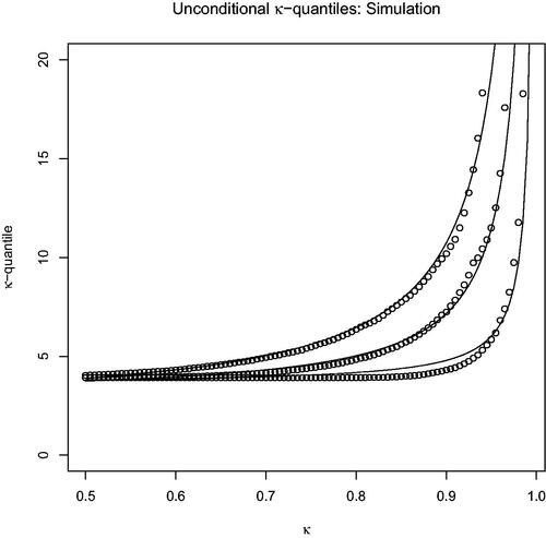
Figure 4 suggests that the unconditional κ-quantiles also grow like $1/(1-\kappa )$ for κ approaching 1. This growth-rate was already observed in Proposition 4 for conditional quantiles. Also, the unconditional κ-quantiles increase as $\left|\right|\beta \left|\right|$ increases, which is again consistent with that proposition. Repeating this simulation for a range of other choices for p, β, and λ gave qualitatively similar results, which are not shown here for the sake of brevity. For these other choices, the corresponding κ-quantiles decrease as the probability of selecting either a very small model or an almost full model increases, and vice versa. This is consistent with our findings from Corollary 1 and Figure 3.

5 Discussion

The polyhedral method can be used whenever the conditioning event of interest can be represented as a polyhedron. And our results can be applied whenever the polyhedral method is used for constructing confidence intervals. Besides the Lasso, this also includes other model selection methods as well as some recent proposals related to the polyhedral method that are mentioned in Remark 3.

By construction, the polyhedral method gives intervals like $[L_{\widehat{m},\widehat{s}},U_{\widehat{m},\widehat{s}}]$ and $[L_{\widehat{m}},U_{\widehat{m}}]$ that are derived from a confidence set based on a truncated univariate distribution (in our case, a truncated normal). Through this, the former intervals are rather easy to compute. And through this, the former intervals are valid conditional on quite small events, namely $\{\widehat{m}=m,\widehat{s}=s,(I_n-P_{{\eta }^m})Y=z\}$ and $\{\widehat{m}=m,(I_n-P_{{\eta }^m})Y=z\}$, respectively, which is a strong property; see Equation (4)(4) $${\mathbb{P}}_{\mu ,{\sigma }^2}({\eta }^{m\prime }\mu \in [L_{m,s}(Y),U_{m,s}(Y)\left]\right|\widehat{m}=m,\widehat{s}=s,(I_n-P_{{\eta }^m})Y=z)=1-\alpha .$$(4) . But through this, the former intervals also inherit the property that their length can be quite large. This undesirable property is inherited through the conditioning on $(I_n-P_{{\eta }^m})Y$. Example 3 in Fithian, Sun, and Taylor (2017) demonstrates that requiring validity only on larger events, like $\{\widehat{m}=m,\widehat{s}=s\}$ or $\{\widehat{m}=m\}$, can result in much shorter intervals. But when conditioning on these larger events, the underlying reference distribution is no longer a univariate truncated distribution but an n-variate truncated distribution. Computations involving the corresponding n-variate cdf are much harder than those in the univariate case.

A recently proposed construction, selective inference with a randomized response, provides higher power of hypothesis tests conditional on the outcome of the model selection step, and hence also improved confidence sets based on these tests; cf. Tian and Taylor (2016) and, in particular, Figure 2 in that reference. This increase in power is obtained by decreasing the “power” of the model selection step itself, in the sense that the model selector $\widehat{m}(y)$ is replaced by $\widehat{m}(y+\omega )$, where ω represents additional randomization that is added to the data. Again, finite-sample computations are demanding in that setting compared to the simple polyhedral method (see Tian and Taylor 2016, sec. 4.2.2).

Another alternative construction, uniformly most accurate unbiased (UMAU) confidence intervals should be mentioned here. When the data-generating distribution belongs to an exponential family, UMAU intervals can be constructed conditional on events of interest like $\{\widehat{m}=m\}$ or on smaller events like $\{\widehat{m}=m,(I_n-P_{{\eta }^m})Y=z\}$; cf. Fithian, Sun, and Taylor (2017). In either case, UMAU intervals require more involved computations than the equal-tailed intervals considered here.

Acknowledgments

We thank the associate editor and two referees, whose feedback has led to significant improvements of the article. Also, helpful input from Nicolai Amann is greatly appreciated.

Appendix A:

Auxiliary Results

In this section, we collect some properties of functions like $F_{\theta ,{\varsigma }^2}^T(w)$ that will be needed in the proofs of Propositions 1 and 2. The following result will be used repeatedly in the following and is easily verified using L’Hospital’s method.

Lemma A.1.

For all a, b with $-\infty \le a<b\le \infty$, the following holds$$\underset{\theta \to \infty }{\lim }\frac{\Phi \left(a-\theta \right)}{\Phi \left(b-\theta \right)}=0.$$

Write $F_{\theta ,{\varsigma }^2}^T(w)$ and $f_{\theta ,{\varsigma }^2}^T(w)$ for the cdf and pdf of the $TN(\theta ,{\varsigma }^2,T)$-distribution, where $T={\cup }_{i=1}^K(a_i,b_i)$ with $-\infty \le a_1<b_1<a_2<\dots <a_K<b_K\le \infty$. For $w\in T$ and for k so that $a_k<w<b_k$, we have$$F_{\theta ,{\varsigma }^2}^T(w)=\frac{\Phi \left(\frac{w-\theta }{\varsigma }\right)-\Phi \left(\frac{a_k-\theta }{\varsigma }\right)+\sum _{i=1}^{k-1}\Phi \left(\frac{b_i-\theta }{\varsigma }\right)-\Phi \left(\frac{a_i-\theta }{\varsigma }\right)}{\sum _{i=1}^K\Phi \left(\frac{b_i-\theta }{\varsigma }\right)-\Phi \left(\frac{a_i-\theta }{\varsigma }\right)};$$if k = 1, the sum in the numerator is to be interpreted as 0. And for w as above, the density $f_{\theta ,{\varsigma }^2}^T(w)$ is equal to $\varphi ((w-\theta )/\varsigma )/\varsigma$ divided by the denominator in the preceding display.

Lemma A.2.

For each fixed $w\in T$, $F_{\theta ,{\varsigma }^2}^T(w)$ is continuous and strictly decreasing in θ, and$$\underset{\theta \to -\infty }{\lim }{F}_{\theta ,{\varsigma }^2}^T(w)=1\hspace{1em}\text{and}\hspace{1em}\underset{\theta \to \infty }{\lim }{F}_{\theta ,{\varsigma }^2}^T(w)=0.$$

Proof.

Continuity is obvious and monotonicity has been shown in Lee et al. (2016) for the case where T is a single interval, that is, K = 1; it is easy to adapt that argument to also cover the case K > 1. Next consider the formula for $F_{\theta ,{\varsigma }^2}^T(w)$. As $\theta \to \infty$, Lemma A.1 implies that the leading term in the numerator is $\Phi ((w-\theta )/\varsigma )$ while the leading term in the denominator is $\Phi ((b_K-\theta )/\varsigma )$. Using Lemma A.1 again gives $\underset{\theta \to \infty }{\lim }{F}_{\theta ,{\varsigma }^2}^T(w)=0$. Finally, it is easy to see that $F_{\theta ,{\varsigma }^2}^T(w)=1-F_{-\theta ,{\varsigma }^2}^{-T}(-w)$ (upon using the relation $\Phi (t)=1-\Phi (-t)$ and a little algebra). With this, we also obtain that $\underset{\theta \to -\infty }{\lim }{F}_{\theta ,{\varsigma }^2}^T(w)=1$. □

For $\gamma \in (0,1)$ and $w\in T$, define $Q_{\gamma }(w)$ through$$F_{Q_{\gamma }(w),{\varsigma }^2}^T(w)=\gamma .$$

Lemma A.2

ensures that $Q_{\gamma }(w)$ is well-defined. Note that $L(w)=Q_{1-\alpha /2}(w)$ and $U(w)=Q_{\alpha /2}(w)$.

Lemma A.3.

For fixed $w\in T,Q_{\gamma }(w)$ is strictly decreasing in γ on (0, 1). And for fixed $\gamma \in (0,1),Q_{\gamma }(w)$ is continuous and strictly increasing in $w\in T$ so that $\underset{w\searrow a_1}{\lim }{Q}_{\gamma }(w)=-\infty$ and $\underset{w\nearrow b_K}{\lim }{Q}_{\gamma }(w)=\infty$.

Proof.

Fix $w\in T$. Strict monotonicity of $Q_{\gamma }(w)$ in γ follows from strict monotonicity of $F_{\theta ,{\varsigma }^2}^T(w)$ in θ; cf. Lemma A.2.

Fix $\gamma \in (0,1)$ throughout the following. To show that $Q_{\gamma }(·)$ is strictly increasing on T, fix $w,w\prime \in T$ with $w<w\prime$. We get$$\gamma =F_{Q_{\gamma }(w),{\varsigma }^2}^T(w)<F_{Q_{\gamma }(w),{\varsigma }^2}^T(w\prime ),$$where the inequality holds because the density of $F_{Q_{\gamma }(w),{\varsigma }^2}^T(·)$ is positive on T. The definition of $Q_{\gamma }(w\prime )$ and Lemma A.2 entail that $Q_{\gamma }(w)<Q_{\gamma }(w\prime )$.

To show that $Q_{\gamma }(·)$ is continuous on T, we first note that $F_{\theta ,{\varsigma }^2}^T(w)$ is continuous in $(\theta ,w)\in \mathbb{R}\times T$ (which is easy to see from the formula for $F_{\theta ,{\varsigma }^2}^T(w)$ given after Lemma A.1). Now fix $w\in T$. Because $Q_{\gamma }(·)$ is monotone, it suffices to show that $Q_{\gamma }(w_n)\to Q_{\gamma }(w)$ for any increasing sequence w_n in T converging to w from below, and for any decreasing sequence w_n converging to w from above. If the w_n increase toward w from below, the sequence $Q_{\gamma }(w_n)$ is increasing and bounded by $Q_{\gamma }(w)$ from above, so that $Q_{\gamma }(w_n)$ converges to a finite limit $\overline{Q}$. With this, and because $F_{\theta ,{\varsigma }^2}^T(w)$ is continuous in $(\theta ,w)$, it follows that$$\underset{n}{\lim }{F}_{Q_{\gamma }(w_n),{\varsigma }^2}^T(w_n)=F_{\overline{Q},{\varsigma }^2}^T(w).$$

In the preceding display, the sequence on the left-hand side is constant equal to γ by definition of $Q_{\gamma }(w_n)$, so that $F_{\overline{Q},{\varsigma }^2}^T(w)=\gamma$. It follows that $\overline{Q}=Q_{\gamma }(w)$. If the w_n decrease toward w from above, a similar argument applies.

To show that $\underset{w\nearrow b_K}{\lim }{Q}_{\gamma }(w)=\infty$, let w_n, $n\ge 1$, be an increasing sequence in T that converges to b_K. It follows that $Q_{\gamma }(w_n)$ converges to a (not necessarily finite) limit $\overline{Q}$ as $n\to \infty$. If $\overline{Q}<\infty$, we get for each $b<b_K$ that$$\underset{n}{\lim \inf }{F}_{Q_{\gamma }(w_n),{\varsigma }^2}^T(w_n)\ge \underset{n}{\lim \inf }{F}_{Q_{\gamma }(w_n),{\varsigma }^2}^T(b)=F_{\overline{Q},{\varsigma }^2}^T(b).$$

In this display, the inequality holds because $F_{Q_{\gamma }(w_n),{\varsigma }^2}^T(·)$ is a cdf, and the equality holds because $F_{\theta ,{\varsigma }^2}^T(b)$ is continuous in θ. As this holds for each $b<b_K$, we obtain that $\underset{n}{\lim \inf }{F}_{Q_{\gamma }(w_n),{\varsigma }^2}^T(w_n)=1$. But in this equality, the left-hand side equals γ—a contradiction. By similar arguments, it also follows that $\underset{w\searrow a_1}{\lim }{Q}_{\gamma }(w)=-\infty$. □

Lemma A.4.

The function $Q_{\gamma }(·)$ satisfies$$\begin{array}{c}\underset{w\nearrow b_K}{\lim }(b_K-w)Q_{\gamma }(w)=-{\varsigma }^2\hspace{0.17em}\text{log}\hspace{0.17em}(\gamma )\text{if}\mathrm{}{b}_K<\infty \mathrm{}\text{and}\\ \underset{w\searrow a_1}{\lim }(a_1-w)Q_{\gamma }(w)=-{\varsigma }^2\hspace{0.17em}\text{log}\hspace{0.17em}(1-\gamma )\text{if}\mathrm{}{a}_1>-\infty .\end{array}$$

Proof. A

s both statements follow from similar arguments, we only give the details for the first one. As w approaches b_K from below, $Q_{\gamma }(w)$ converges to $\infty$ by Lemma A.3. This observation, the fact that $F_{Q_{\gamma }(w),{\varsigma }^2}^T(w)=\gamma$ holds for each w, and Lemma A.1 together imply that$$\underset{w\nearrow b_K}{\lim }\frac{\Phi \left(\frac{w-Q_{\gamma }(w)}{\varsigma }\right)}{\Phi \left(\frac{b_K-Q_{\gamma }(w)}{\varsigma }\right)}=\gamma .$$

Because $\Phi (-x)/(\varphi (x)/x)\to 1$ as $x\to \infty$ (cf. Feller 1957, Lemma VII.1.2.), we get that$$\underset{w\nearrow b_K}{\lim }\frac{\varphi \left(\frac{w-Q_{\gamma }(w)}{\varsigma }\right)}{\varphi \left(\frac{b_K-Q_{\gamma }(w)}{\varsigma }\right)}=\gamma .$$

The claim now follows by plugging-in the formula for $\varphi (·)$ on the left-hand side, simplifying, and then taking the logarithm of both sides. □

Appendix B

Proof of Proposition 1

Proof

of the first statement in Proposition 1. Assume that $b_K<\infty$ (the case where $a_1>-\infty$ is treated similarly). Lemma A.4 entails that $\underset{w\nearrow b_K}{\lim }(b_K-w)(U(w)-L(w))={\varsigma }^{2}C$, where $C=\hspace{0.17em}\text{log}\hspace{0.17em}((1-\alpha /2)/(\alpha /2))$ is positive. Hence, there exists a constant $ϵ>0$ so that$$U(w)-L(w)>\frac{1}{2}\frac{{\varsigma }^{2}C}{b_K-w}$$whenever $w\in (b_K-ϵ,b_K)\cap T$. Set $B=\inf \{f_{\theta ,{\varsigma }^2}^T(w):w\in (b_K-ϵ,b_K)\cap T\}$. For $w\in T$, $f_{\theta ,{\varsigma }^2}^T(w)$ is a Gaussian density divided by a constant scaling factor, so that B > 0. Because $U(w)-L(w)\ge 0$ in view of Lemma A.3, we obtain that$${\mathbb{E}}_{\theta ,{\varsigma }^2}[U(W)-L(W)|W\in T]\ge \frac{{\varsigma }^{2}BC}{2}{\int }_{(b_K-ϵ,b_K)\cap T}\frac{1}{b_K-w}dw=\infty .$$

□

Proof

of the first inequality in Proposition 1. Define $R_{\gamma }(w)$ through $\Phi ((w-R_{\gamma }(w))/\varsigma )=\gamma$, that is, $R_{\gamma }(w)=w-\varsigma {\Phi }^{-1}(\gamma )$ Then, on the one hand, we have$$\begin{array}{c}{F}_{R_{\gamma }(w),{\varsigma }^2}^T(w)=\frac{P(N(R_{\gamma }(w),{\varsigma }^2)\le w,N(R_{\gamma }(w),{\varsigma }^2)\in T)}{P(N(R_{\gamma }(w),{\varsigma }^2)\in T)}\\ \le \frac{P(N(R_{\gamma }(w),{\varsigma }^2)\le w)}{\underset{\vartheta }{\inf }P(N(\vartheta ,{\varsigma }^2)\in T)}=\frac{\gamma }{p_{\ast }},\end{array}$$while, on the other,$$\begin{array}{c}{F}_{R_{\gamma }(w),{\varsigma }^2}^T(w)\ge \frac{P(N(R_{\gamma }(w),{\varsigma }^2)\le w)-P(N(R_{\gamma }(w),{\varsigma }^2)\notin T)}{P(N(R_{\gamma }(w),{\varsigma }^2)\in T)}\\ \ge \underset{\vartheta }{\inf }\frac{P(N(R_{\gamma }(w),{\varsigma }^2)\le w)-1+P(N(\vartheta ,{\varsigma }^2)\in T)}{P(N(\vartheta ,{\varsigma }^2)\in T)}\\ =\frac{\gamma -1+p_{\ast }}{p_{\ast }}.\end{array}$$

The inequalities in the preceding two displays imply that$$R_{1-p_{\ast }(1-\gamma )}(w)\le Q_{\gamma }(w)\le R_{p_{\ast }\gamma }(w).$$

(Indeed, the inequality in the third-to-last display continues to hold with $p_{\ast }\gamma$ replacing γ; in that case, the upper bound reduces to γ; similarly, the inequality in the second-to-last display continues to hold with $1-p_{\ast }(1-\gamma )$ replacing γ, in which case the lower bound reduces to γ. Now use the fact that $F_{\theta ,{\varsigma }^2}^T(w)$ is decreasing in θ.) In particular, we get that $U(w)=Q_{\alpha /2}(w)\le R_{p_{\ast }\alpha /2}(w)=w-\varsigma {\Phi }^{-1}(p_{\ast }\alpha /2)$ and that $L(w)=Q_{1-\alpha /2}(w)\ge R_{1-p_{\ast }\alpha /2}(w)=w-\varsigma {\Phi }^{-1}(1-p_{\ast }\alpha /2)$. The last two inequalities, and the symmetry of $\Phi (·)$ around zero, imply the first inequality in the proposition. □

Proof

of the second inequality in Proposition 1. Note that $p_{\ast }\ge p_{°}=\underset{\vartheta }{\inf }P(N(\vartheta ,{\varsigma }^2)<b_1\mathrm{}\text{or}\mathrm{}N(\vartheta ,{\varsigma }^2)>a_K)$, because T is unbounded above and below. Setting $\delta =(a_K-b_1)/(2\varsigma )$, we note that $\delta \ge 0$ and that it is elementary to verify that $p_{°}=2\Phi (-\delta )$. Because ${\Phi }^{-1}(1-p_{\ast }\alpha /2)\le {\Phi }^{-1}(1-p_{°}\alpha /2)$, the inequality will follow if we can show that ${\Phi }^{-1}(1-p_{°}\alpha /2)\le {\Phi }^{-1}(1-\alpha /2)+\delta$ or, equivalently, that ${\Phi }^{-1}(p_{°}\alpha /2)\ge {\Phi }^{-1}(\alpha /2)-\delta$. Because $\Phi (·)$ is strictly increasing, this is equivalent to$$p_{°}\alpha /2=\Phi (-\delta )\alpha \ge \Phi ({\Phi }^{-1}(\alpha /2)-\delta ).$$

To this end, we set $f(\delta )=\alpha \Phi (-\delta )/\Phi ({\Phi }^{-1}(\alpha /2)-\delta )$ and show that $f(\delta )\ge 1$ for $\delta \ge 0$. Because $f(0)=1$, it suffices to show that $f\prime (\delta )$ is nonnegative for $\delta >0$. The derivative can be written as a fraction with positive denominator and with numerator equal to$$-\alpha \varphi (-\delta )\Phi ({\Phi }^{-1}(\alpha /2)-\delta )+\alpha \Phi (-\delta )\varphi ({\Phi }^{-1}(\alpha /2)-\delta ).$$

The expression in the preceding display is nonnegative if and only if$$\frac{\Phi (-\delta )}{\varphi (-\delta )}\ge \frac{\Phi ({\Phi }^{-1}(\alpha /2)-\delta )}{\varphi ({\Phi }^{-1}(\alpha /2)-\delta )}.$$

This will follow if the function $g(x)=\Phi (-x)/\varphi (x)$ is decreasing in $x\ge 0$. The derivative $g\prime (x)$ can be written as a fraction with positive denominator and with numerator equal to$$-\varphi {(x)}^2+x\Phi (-x)\varphi (x)=x\varphi (x)\left(\Phi (-x)-\frac{\varphi (x)}{x}\right).$$

Using the well-known inequality $\Phi (-x)\le \varphi (x)/x$ for x > 0 (Feller 1957, Lemma VII.1.2.), we see that the expression in the preceding display is nonpositive for x > 0. □

Appendix C

Proof of Proposition 2

From Lee et al. (2016), we recall the formulas for the expressions on the right-hand side of (2), namely $A_{m,s}=(A_{m,s}^0\prime ,A_{m,s}^1\prime )\prime$ and $b_{m,s}=(b_{m,s}^0\prime ,b_{m,s}^1\prime )\prime$ with $A_{m,s}^0$ and $b_{m,s}^0$ given by$$\frac{1}{\lambda }\left(\begin{array}{c}{X}_{m^c}{}^{\prime }(I_n-P_{X_m})\\ -X_{m^c}{}^{\prime }(I_n-P_{X_m})\end{array}\right)\hspace{1em}\text{and}\hspace{1em}\left(\begin{array}{c}\iota -X_{m^c}{}^{\prime }{X}_m{(X_{m^{\prime }}{X}_m)}^{-1}s\\ \iota +X_{m^c}{}^{\prime }{X}_m{(X_{m^{\prime }}{X}_m)}^{-1}s\end{array}\right),$$respectively, and with $A_{m,s}^1=-\text{diag}(s){(X_m^{\prime }{X}_m)}^{-1}{X}_m^{\prime }$ and $b_{m,s}^1=-\lambda \text{diag}(s){(X_m^{\prime }{X}_m)}^{-1}s$ (in the preceding display, $P_{X_m}$ denotes the orthogonal projection matrix onto the column space spanned by X_m and ι denotes an appropriate vector of ones). Moreover, it is easy to see that the set $\{y:A_{m,s}y<b_{m,s}\}$ can be written as $\{y:\mathrm{}\text{for}\mathrm{}z=(I_p-P_{{\eta }^m})y$, we have ${\mathcal{V}}_{m,s}^{-}(z)<{\eta }^{m\prime }y<{\mathcal{V}}_{m,s}^{+}(z),{\mathcal{V}}_{m,s}^0(z)>0\}$, where$$\begin{array}{c}{\mathcal{V}}_{m,s}^{-}(z)=\max (\{{(b_{m,s}-A_{m,s}z)}_i/{(A_{m,s}{c}^m)}_i:{(A_{m,s}{c}^m)}_i<0\}\cup \{-\infty \}),\\ {\mathcal{V}}_{m,s}^{+}(z)=\min (\{{(b_{m,s}-A_{m,s}z)}_i/{(A_{m,s}{c}^m)}_i:{(A_{m,s}{c}^m)}_i>0\}\cup \{\infty \}),\\ {\mathcal{V}}_{m,s}^0(z)=\min (\{{(b_{m,s}-A_{m,s}z)}_i:{(A_{m,s}{c}^m)}_i=0\}\cup \{\infty \})\end{array}$$

with $c^m={\eta }^m/\left|\right|{\eta }^m|{|}^2$; cf. also Lee et al. (2016).

Proof of Proposition 2.

Set $I_{-}=\{i:{(A_{m,s}{c}^m)}_i<0\}$ and $I_{+}=\{i:{(A_{m,s}{c}^m)}_i>0\}$. In view of the formulas of ${\mathcal{V}}_{m,s}^{-}(z)$ and ${\mathcal{V}}_{m,s}^{+}(z)$ given earlier, it suffices to show that either $I_{-}$ or $I_{+}$ is nonempty. Conversely, assume that $I_{-}=I_{+}=\varnothing$. Then $A_{m,s}{c}^m=0$ and hence also $A_{m,s}^1{c}^m=0$. Using the explicit formula for $A_{m,s}^1$ and the definition of η^m, that is, ${\eta }^m=X_m{(X_m^{\prime }{X}_m)}^{-1}{\gamma }^m$, it follows that ${\gamma }^m=0$, which contradicts our assumption that ${\gamma }^m\in {\mathbb{R}}^{\left|m\right|}\setminus \left\{0\right\}$. □

Appendix D

Proof of Proposition 3 and Corollary 1

As a preparatory consideration, recall that $T_m((I_n-P_{{\eta }^m})y)$ is the union of the intervals $({\mathcal{V}}_{m,s}^{-}((I_n-P_{{\eta }^m})y),{\mathcal{V}}_{m,s}^{+}((I_n-P_{{\eta }^m})y))$ with $s\in {\mathcal{S}}_m^{+}$. Inspection of the explicit formulas for the interval endpoints given in Appendix C now immediately reveals the following: The lower endpoint ${\mathcal{V}}_{m,s}^{-}((I_n-P_{{\eta }^m})y)$ is either constant equal to $-\infty$ on the set $\{y:A_{m,s}y<b_{m,s}\}$, or it is the minimum of a finite number of linear functions of y (and hence finite and continuous) on that set. Similarly the upper endpoint ${\mathcal{V}}_{m,s}^{+}((I_n-P_{{\eta }^m})y)$ is either constant equal to $\infty$ on that set, or it is the maximum of a finite number of linear functions of y (and hence finite and continuous) on that set.

Proof of Proposition 3.

Let $m\in {\mathcal{M}}^{+}\setminus \{\varnothing \}$. We first assume, for some s and y with $s\in {\mathcal{S}}_m^{+}$ and $A_{m,s}y<b_{m,s}$, that the set in (6) is bounded from above (the case of boundedness from below is similar). Then there is an open neighborhood O of y, so that each point $w\in O$ satisfies $A_{m,s}w<b_{m,s}$ and also so that $T_m((I_n-P_{{\eta }^m})w)$ is bounded from above. Because O has positive Lebesgue measure, (5) now follows from Proposition 1. To prove the converse, assume for each $s\in {\mathcal{S}}_m^{+}$ and each y satisfying $A_{m,s}y<b_{m,s}$ that $T_m((I_n-P_{{\eta }^m})y)$ is unbounded from above and from below. Because the sets $\{y:A_{m,s}y<b_{m,s}\}$ for $s\in {\mathcal{S}}_m^{+}$ are disjoint by construction, the same is true for the sets $T_{m,s}((I_n-P_{{\eta }^m})y)$ for $s\in {\mathcal{S}}_m^{+}$. Using Proposition 1, we then obtain that $U_{\widehat{m}}(Y)-L_{\widehat{m}}(Y)$ is bounded by a linear function of$$\max \{{\mathcal{V}}_{m,s}^{-}((I_n-P_{{\eta }^m})Y):s\in {\mathcal{S}}_m^{+}\}-\min \{{\mathcal{V}}_{m,s}^{+}((I_n-P_{{\eta }^m})Y):s\in {\mathcal{S}}_m^{+}\}$$

Lebesgue-almost everywhere on the event $\{\widehat{m}=m\}$. (The maximum and the minimum in the preceding display correspond to a_K and b₁, respectively, in Proposition 1.) It remains to show that the expression in the preceding display has finite conditional expectation on the event $\{\widehat{m}=m\}$. But this expression is the maximum of a finite number of Gaussians minus the minimum of a finite number of Gaussians. Its unconditional expectation, and hence also its conditional expectation on the event $\{\widehat{m}=m\}$, is finite. □

Proof of Corollary 1.

The statement for $\left|m\right|=0$ is trivial. Next, consider the case where $\left|m\right|=1$. Take $s\in {\mathcal{S}}_m^{+}$ and y so that $A_{m,s}y<b_{m,s}$. We need to show that $T_m(z)=T_{m,-1}(z)\cup T_{m,1}(z)$ is unbounded above and below for $z=(I_n-P_{{\eta }^m})y$. To this end, first recall the formulas presented at the beginning of Appendix C. Together with the fact that, here, ${\eta }^m=X_m{\gamma }^m/\left|\right|X_m|{|}^2\ne 0$, these formulas entail that $A_{m,1}^0{c}^m=A_{m,-1}^0{c}^m=0$ and that $A_{m,1}^1{c}^m=-A_{m,-1}^1{c}^m\ne 0$. With this, and in view of the definitions of ${\mathcal{V}}_{m,s}^{-}(z)$, ${\mathcal{V}}_{m,s}^{+}(z)$ and ${\mathcal{V}}_{m,s}^0(z)$ in Appendix C, it follows that $T_m(z)$ is a set of the form $(-\infty ,-a)\cup (a,\infty )$, which is unbounded.

Finally, assume that $\left|m\right|=p\le n$. Fix $s\in {\mathcal{S}}_m^{+}$ and y so that $A_{m,s}y<b_{m,s}$, and set $z=(I_n-P_{{\eta }^m})y$. Again, we need to show that $T_m(z)={\cup }_{\tilde{s}\in {\mathcal{S}}_m^{+}}{T}_{m,\tilde{s}}(z)$ is unbounded above and below. For each $\tilde{s}\in {\mathcal{S}}_m^{+}$, it is easy to see that $A_{m,\tilde{s}}^0{c}^m=0$ and that $b_{m,\tilde{s}}^0$ is a vector of ones. The condition $A_{m,\tilde{s}}y<b_{m,\tilde{s}}$ hence reduces to $A_{m,\tilde{s}}^{1}y<b_{m,\tilde{s}}^1$. Note that $A_{m,\tilde{s}}^1{c}^m=-\text{diag}(\tilde{s}){(X_m^{\prime }{X}_m)}^{-1}{\gamma }^m/{\gamma }^{m\prime }{(X_m^{\prime }{X}_m)}^{-1}{\gamma }^m$, and that the set of its zero-components does not depend on $\tilde{s}$. We henceforth assume that γ^m is such that all components of $A_{m,s}^1{c}^m$ are nonzero, which is satisfied for Lebesgue-almost all vectors γ^m. Now choose sign-vectors s⁺ and s^– in ${\{-1,1\}}^p$ as follows: Set $s_i^{+}=-1$ if ${(A_{m,s}^1{c}^m)}_i<0$; otherwise, set $s_i^{+}=s_i$. With this, we get that $A_{m,s^{+}}{c}^m$ is a nonzero vector with positive components. Choose s^– in a similar fashion, so that $A_{m,s^{-}}{c}^m$ is a nonzero vector with negative components. It follows that $T_{m,s^{+}}(z)\cup T_{m,s^{-}}(z)$ is a set of the form $(-\infty ,-a)\cup (a,\infty )$. We next show that s⁺ and s^– lie in ${\mathcal{S}}_m^{+}$. Choose y⁺ so that $(I_n-P_{{\eta }^m})y^{+}=z$ and so that ${\eta }^{m\prime }{y}^{+}\in T_{m,s}^{+}(z)$. Because ${\mathcal{V}}_{m,s^{+}}^0(z)=\infty$ by construction, it follows that $A_{m,s^{+}}{y}^{+}<b_{m,s^{+}}$ and hence $\widehat{m}(y^{+})=m$ and $\widehat{s}(y^{+})=s^{+}$. Because the same is true for all points in a sufficiently small open ball around y⁺, the event $\{\widehat{m}=m,\widehat{s}=s^{+}\}$ has positive probability and hence $s^{+}\in {\mathcal{S}}_m^{+}$. A similar argument entails that $s^{-}\in {\mathcal{S}}_m^{+}$. Taken together, we see that $T_{m,s^{+}}(z)\cup T_{m,s^{-}}(z)\subseteq {\cup }_{\tilde{s}\in {\mathcal{S}}_m^{+}}{T}_{m,\tilde{s}}(z)=T_m(z)$, so that the last set is indeed unbounded above and below. □

Remark D.1.

The statement in Corollary 1 for the case $\left|m\right|=p\le n$ does not hold for all γ^m or, equivalently, for all η^m. For example, if γ^m is such that η^m is parallel to one of the columns of X, then some components of $A_{m,s}^1{c}^m$ are zero and $T_m((I_n-P_{{\eta }^m})y)$ can be bounded for some y. Figure D1 illustrates the situation.

Appendix E

Proof of Proposition 4

We only consider the case where $b=\sup T<\infty$; the case where $a=\inf T>-\infty$ is treated similarly. The proof relies on the observation that$$\underset{w\nearrow b}{\lim }\frac{U(w)-L(w)}{A(w)}=1$$for $A(w)={\varsigma }^2\frac{\hspace{0.17em}\text{log}\hspace{0.17em}((2-\alpha )/\alpha )}{b-w}$ in view of Lemma A.4. The quantiles of A(W) are easy to compute: If $s_{\theta ,{\varsigma }^2}(\kappa )$ denotes the κ-quantile of A(W), then$$s_{\theta ,{\varsigma }^2}(\kappa )=\frac{{\varsigma }^2\hspace{0.17em}\text{log}\hspace{0.17em}((2-\alpha )/\alpha )}{b-F_{\theta ,{\varsigma }^2}^{T^{-1}}(\kappa )}.$$

The denominator in the preceding display, which involves the inverse of $F_{\theta ,{\varsigma }^2}^T(·)$, can be approximated as follows.

Lemma

E.1. For $\kappa \nearrow 1$, we have$$b-F_{\theta ,{\varsigma }^2}^{T^{-1}}(\kappa )=(1-\kappa )\varsigma \frac{P(V\in T)}{\varphi ((b-\theta )/\varsigma )}(1+o(1)),$$where $V\sim N(\theta ,{\varsigma }^2)$.

Proof.

With the convention that $F_{\theta ,{\varsigma }^2}^{T^{-1}}(1)=b$ and as $\kappa \nearrow 1$, we have$$\begin{array}{c}b-F_{\theta ,{\varsigma }^2}^{T^{-1}}(\kappa )=F_{\theta ,{\varsigma }^2}^{T^{-1}}(1)-F_{\theta ,{\varsigma }^2}^{T^{-1}}(\kappa )=(1-\kappa )\frac{F_{\theta ,{\varsigma }^2}^{T^{-1}}(1-(1-\kappa ))-F_{\theta ,{\varsigma }^2}^{T^{-1}}(1)}{-(1-\kappa )}\\ =(1-\kappa )\left((F_{\theta ,{\varsigma }^2}^{T^{-1}})\prime (1-)+o(1)\right)=(1-\kappa )(F_{\theta ,{\varsigma }^2}^{T^{-1}})\prime (1-)(1+o(1))\\ =(1-\kappa )\frac{1}{(F_{\theta ,{\varsigma }^2}^T)\prime (b-)}(1+o(1))=(1-\kappa )\frac{P(V\in T)}{{\varsigma }^{-1}\varphi ((b-\theta )/\varsigma )}(1+o(1)),\end{array}$$where the second-to-last equality relies on the inverse function theorem and the last equality holds because $F_{\theta ,{\varsigma }^2}^T(w)=P(V\le w|V\in T)$. □

Lemma

E.2. The κ-quantiles of A(W) provide an asymptotic lower bound for the κ-quantiles of the length $U(W)-L(W)$, in the sense that $\underset{\kappa \nearrow 1}{\lim \sup }{s}_{\theta ,{\varsigma }^2}(\kappa )/q_{\theta ,{\varsigma }^2}(\kappa )\le 1$.

Proof.

Fix $ϵ\in (0,1)$ and choose $\delta >0$ so that $(1-ϵ)A(w)\le U(w)-L(w)$ whenever $w\in (b-\delta ,b)$. In addition, we may assume that δ is sufficiently small so that the cdf of W is strictly increasing on $(b-\delta ,b)$. Using the formula for A(W), we get that$$\{A(W)>x\}=\{W>b-\frac{{\varsigma }^2\hspace{0.17em}\text{log}\hspace{0.17em}((2-\alpha )/\alpha )}{x}\}$$for x > 0. By Lemma E.1, $s_{\theta ,{\varsigma }^2}(\kappa )$ converges to infinity as $\kappa \nearrow 1$. Hence, we have $\frac{{\varsigma }^2\hspace{0.17em}\text{log}\hspace{0.17em}((2-\alpha )/\alpha )}{s_{\theta ,{\varsigma }^2}(\kappa )}<\delta /2$ for κ sufficiently close to 1, say, $\kappa \in ({\kappa }_0,1)$. For each $\rho \in (1/2,1)$ and $\kappa \in ({\kappa }_0,1)$, we obtain that$$\begin{array}{c}\{A(W)>\rho s_{\theta ,{\varsigma }^2}(\kappa )\}=\{A(W)>\rho s_{\theta ,{\varsigma }^2}(\kappa ),W>b-\delta \}\\ \hspace{1em}\subseteq \{U(W)-L(W)>(1-ϵ)\rho s_{\theta ,{\varsigma }^2}(\kappa )\},\end{array}$$

which entails that$$P\left(U(W)-L(W)\le (1-ϵ)\rho s_{\theta ,{\varsigma }^2}(\kappa )\right)<\kappa$$because the cdf of W strictly increases from $\rho s_{\theta ,{\varsigma }^2}(\kappa )$ to $s_{\theta ,{\varsigma }^2}(\kappa )$. It follows that $(1-ϵ)\rho s_{\theta ,{\varsigma }^2}(\kappa )\le q_{\theta ,{\varsigma }^2}(\kappa )$ whenever $\rho \in (1/2,1)$ and $\kappa \in ({\kappa }_0,1)$. Letting ρ go to 1 gives $(1-ϵ)s_{\theta ,{\varsigma }^2}(\kappa )\le q_{\theta ,{\varsigma }^2}(\kappa )$ whenever $\kappa \in ({\kappa }_0,1)$. Hence, $\underset{\kappa \nearrow 1}{\lim \sup }(1-ϵ)s_{\theta ,{\varsigma }^2}(\kappa )/q_{\theta ,{\varsigma }^2}(\kappa )\le 1$. Since $ϵ$ can be chosen arbitrarily close to zero, this completes the proof. □

Proof of Proposition 4.

Use the formula for $s_{\theta ,{\varsigma }^2}(\kappa )$ and Lemma E.1 to obtain that$$\begin{array}{c}\frac{s_{\theta ,{\varsigma }^2}(\kappa )}{q_{\theta ,{\varsigma }^2}(\kappa )}=\frac{1}{q_{\theta ,{\varsigma }^2}(\kappa )}\frac{\varsigma \hspace{0.17em}\text{log}\hspace{0.17em}((2-\alpha )/\alpha )}{1-\kappa }\frac{\varphi ((b-\theta )/\varsigma )}{P(V\in T)}(1+o(1))\\ \ge \frac{1}{q_{\theta ,{\varsigma }^2}(\kappa )}\frac{\varsigma \hspace{0.17em}\text{log}\hspace{0.17em}((2-\alpha )/\alpha )}{1-\kappa }\frac{\varphi ((b-\theta )/\varsigma )}{\Phi ((b-\theta )/\varsigma )}(1+o(1))\\ =\frac{r_{\theta ,{\varsigma }^2}(\kappa )}{q_{\theta ,{\varsigma }^2}(\kappa )}(1+o(1))\end{array}$$

as $\kappa \nearrow 1$ (the inequality holds because $T\subseteq (-\infty ,b)$). The claim now follows from this and Lemma E.2. □

Remark.

The argument presented here can be extended to obtain an explicit formula for the exact rate of $q_{\theta ,{\varsigma }^2}(\kappa )$ as $\kappa \nearrow 1$ or as $\theta \to \infty$ (or both). The resulting expression is more involved (the cases where T is bounded from one side and from both sides need separate treatment) but qualitatively similar to $r_{\theta ,{\varsigma }^2}(\kappa )$, as far as its behavior for $\kappa \nearrow 1$ or $\theta \to \infty$ is concerned. In view of this and for the sake of brevity, results for the exact rate are not presented here.

References

- Bachoc, F., Leeb, H., and Pötscher, B. M. (2019), “Valid Confidence Intervals for Post-Model-Selection Predictors,” The Annals of Statistics, 47, 1475–1504. DOI: https://doi.org/10.1214/18-AOS1721.
- Berk, R., Brown, L., Buja, A., Zhang, K., and Zhao, L. (2013), “Valid Post-Selection Inference,” The Annals of Statistics, 41, 802–837. DOI: https://doi.org/10.1214/12-AOS1077.
- Feller, W. (1957), An Introduction to Probability Theory and Its Applications (Vol. 1, 2nd ed.), New York: Wiley.
- Fithian, W., Sun, D., and Taylor, J. (2017), “Optimal Inference After Model Selection,” arXiv no. 1410.2597.
- Fithian, W., Taylor, J., Tibshirani, R., and Tibshirani, R. J. (2015), “Selective Sequential Model Selection,” arXiv no. 1512.02565.
- Frank, I. E., and Friedman, J. H. (1993), “A Statistical View of Some Chemometrics Regression Tools,” Technometrics, 35, 109–135. DOI: https://doi.org/10.1080/00401706.1993.10485033.
- Gross, S. M., Taylor, J., and Tibshirani, R. (2015), “A Selective Approach to Internal Inference,” arXiv no. 1510.00486.
- Lee, J. D., Sun, D. L., Sun, Y., and Taylor, J. (2016), “Exact Post-Selection Inference, With Application to the Lasso,” The Annals of Statistics, 44, 907–927. DOI: https://doi.org/10.1214/15-AOS1371.
- Leeb, H., and Kabaila, P. (2017), “Admissibility of the Usual Confidence Set for the Mean of a Univariate or Bivariate Normal Population: The Unknown Variance Case,” Journal of the Royal Statistical Society, Series B, 79, 801–813. DOI: https://doi.org/10.1111/rssb.12186.
- Leeb, H., and Pötscher, B. M. (2006a), “Can One Estimate the Conditional Distribution of Post-Model-Selection Estimators?,” The Annals of Statistics, 34, 2554–2591. DOI: https://doi.org/10.1214/009053606000000821.
- Leeb, H., and Pötscher, B. M. (2006b), “Performance Limits for Estimators of the Risk or Distribution of Shrinkage-Type Estimators, and Some General Lower Risk-Bound Results,” Econometric Theory, 22, 69–97.
- Leeb, H., and Pötscher, B. M. (2008), “Can One Estimate the Unconditional Distribution of Post-Model-Selection Estimators?,” Econometric Theory, 24, 338–376.
- Markovic, J., Xia, L., and Taylor, J. (2018), “Unifying Approach to Selective Inference With Applications to Cross-Validation,” arXiv no. 1703.06559.
- Panigrahi, S., and Taylor, J. (2019), “Approximate Selective Inference via Maximum-Likelihood,” arXiv no. 1902.07884.
- Panigrahi, S., Zhu, J., and Sabatti, C. (2018), “Selection-Adjusted Inference: An Application to Confidence Intervals for cis-eQTL Effect Sizes,” arXiv no. 1801.08686.
- Pötscher, B. M. (2009), “Confidence Sets Based on Sparse Estimators Are Necessarily Large,” Sankhyā, Series A, 71, 1–18.
- Pötscher, B. M., and Schneider, U. (2010), “Confidence Sets Based on Penalized Maximum Likelihood Estimators in Gaussian Regression,” Electronic Journal of Statistics, 4, 334–360. DOI: https://doi.org/10.1214/09-EJS523.
- Reid, S., Taylor, J., and Tibshirani, R. (2015), “Post-Selection Point and Interval Estimation of Signal Sizes in Gaussian Samples,” arXiv no. 1405.3340.
- Schneider, U. (2016), “Confidence Sets Based on Thresholding Estimators in High-Dimensional Gaussian Regression Models,” Econometric Reviews, 35, 1412–1455. DOI: https://doi.org/10.1080/07474938.2015.1092798.
- Taylor, J., and Tibshirani, R. (2018), “Post-Selection Inference for l1-Penalized Likelihood Models,” Canadian Journal of Statistics, 46, 41–61. DOI: https://doi.org/10.1002/cjs.11313.
- Tian, X., Loftus, J. R., and Taylor, J. (2017), “Selective Inference With Unknown Variance via the Square-Root LASSO,” arXiv no. 1504.08031.
- Tian, X., Panigrahi, S., Markovic, J., Bi, N., and Taylor, J. (2016), “Selective Sampling After Solving a Convex Problem,” arXiv no. 1609. 05609.
- Tian, X., and Taylor, J. (2016), “Selective Inference With a Randomized Response,” arXiv no. 1507.06739.
- Tian, X., and Taylor, J. (2017), “Asymptotics of Selective Inference,” Scandinavian Journal of Statistics, 44, 480–499.
- Tibshirani, R. (1996), “Regression Shrinkage and Selection via the Lasso,” Journal of the Royal Statistical Society, Series B, 58, 267– 288. DOI: https://doi.org/10.1111/j.2517-6161.1996.tb02080.x.
- Tibshirani, R. J. (2013), “The Lasso Problem and Uniqueness,” Electronic Journal of Statistics, 7, 1456–1490. DOI: https://doi.org/10.1214/13-EJS815.
- Tibshirani, R. J., Taylor, J., Lockhart, R., and Tibshirani, R. (2016), “Exact Post-Selection Inference for Sequential Regression Procedures,” Journal of the American Statistical Association, 111, 600–620. DOI: https://doi.org/10.1080/01621459.2015.1108848.