Discussion of Professor Bradley Efron’s Article on “Prediction, Estimation, and Attribution”

1 Introduction

By noting the rapid growing trend of “pure prediction algorithms,” Professor Efron compares and bridges the statistics of the 20th Century (estimation and attribution) to that of the current fast growing development of the 21st Century (prediction). The outstanding discussion offers many deep-rooted insights and comments. As did his forward thinking article on Fisher’s influence on modern statistics (Efron 1998), which helped shape many recent developments on statistical inference (including our own work on confidence distribution (Singh, Xie, and Strawderman 2005; Xie and Singh 2013)), this equally inspiring article by Professor Efron will certainly galvanize many contemporary and powerful developments for modern statistics and for the foundations of data science.

In this note, we echo and also provide additional support to two important points made by Professor Efron: (1) prediction is “an easier task than either attribution or estimation”; (2) the IID assumption (e.g. random splitting of training and testing datasets) is crucial in the current developments on predictions, but we also need to do more for the case when the IID assumption is not met. Based on our own research, we provide additional evidence to support these discussions. We discover that prediction has a homeostasis property and works well under the IID setting even if the learning model used is completely wrong. We also highlight the importance of having a good modeling and inference practice: a good learning model with good estimation is important to improve prediction efficiency in the IID case and it becomes essential to maintain validity in the non-IID case. The message remains: we still need to make effort to build a good learning model and estimation algorithm in prediction, even if prediction is an easier task than estimation.

From the outset, we would like to point out that it is not a straw-man argument to consider non-IID testing data. On the contrary, such data are prevalent in data science. In addition to those examples provided by Professor Efron that showed “drift,” we can easily imagine non-IID examples in many typical applications. For instance, a predictive algorithm is trained on a database of patient medical records and we would like to predict potential outcomes of a treatment for a new patient with more severe symptoms than what the average patient shows. The new patient with more severe symptoms is not a typical IID draw from the general patient population. Similarly, in the finance sector, one is often interested in predicting the financial performance of a particular company. If a predictive model is trained on all institutes, then the testing data (of the specific company of interest) are unlikely IID draws from the same general population of the training data. The limitation of the IID assumption, in our opinion, has hampered our efforts to fully take advantage of fast-developing machine learning methodologies (e.g., deep neural network model, tree based methods, etc.) in many real-world applications.

Our discussions in this note are based on a so-called conformal prediction procedure, an attractive new prediction framework that is error (or model) distribution free (see, e.g., Vovk, Gammerman, and Shafer 2005; Shafer and Vovk 2008). We discover a homeostasis phenomenon that the expected bias caused by using a wrong model can largely be offset by the corresponding negatively shifted predictive errors under the IID setting. Thus, the predictive conclusion is always valid even if the model used to train the data is completely wrong. This robustness result clearly supports the claim that prediction is an easier task than modeling and estimation. However, the use of a wrong training (learning) model has at least two undesirable impacts on prediction: (a) a prediction based on a wrong model typically produces much wider predictive intervals than those based on a correct model; (b) although the IID case enjoys a nice homeostatic cancellation of bias (in fitted model) and shifts (in associated predictive errors) when using a wrong learning model, in the non-IID case this cancellation is often no longer effective, resulting in invalid predictions. The use of a correct learning model can help mitigate and sometimes solve the problem of invalid prediction for non-IID (e.g., drifted or individual-specific) testing data.

Section 2 reviews a conformal predictive procedure and shows that the prediction is valid under the IID setting, even if the learning model is completely wrong. Section 3 is a numerical study using a neural network model to demonstrate the impact of a wrong learning model and estimation on prediction in both the IID and non-IID cases. Section 4 is a concluding remark. A more detailed discussion, including an introduction of predictive curve (to represent predictive intervals of all levels) and an elaborated study of linear models, is in Xie and Zheng (2020).

2 Prediction, Testing Data, and Learning Models

As in Equation (6.4) of Professor Efron’s article, we assume that a training (observed) dataset of size n, say, ${\mathcal{D}}_{\mathrm{ }\text{obs}}=\{({\mathbf{x}}_i,y_i),i=1,\dots ,n\}$ is available, where $({\mathbf{x}}_i,y_i),i=1,\dots ,n$, are IID random samples from an unknown population $\mathcal{F}$. For a given ${\mathbf{x}}_{\mathrm{ }\text{new}}$, we would like to predict what $y_{\mathrm{ }\text{new}}$ would be. We first use the typical assumption that $({\mathbf{x}}_{\mathrm{ }\text{new}},y_{\mathrm{ }\text{new}})$ is also an IID draw from $\mathcal{F}$. Later we relax this requirement and only assume that $y_{\mathrm{ }\text{new}}|{\mathbf{x}}_{\mathrm{ }\text{new}}$ relates to ${\mathbf{x}}_{\mathrm{ }\text{new}}$ the same way as $y_i|{\mathbf{x}}_i$ relates to ${\mathbf{x}}_i$, but ${\mathbf{x}}_{\mathrm{ }\text{new}}$ follows a marginal distribution that is different from that of ${\mathbf{x}}_i$.

For notation convenience, we consider $({\mathbf{x}}_{\mathrm{ }\text{new}},y_{\mathrm{ }\text{new}})$ as the $(n+1)$th observation and introduce the index n + 1, with ${\mathbf{x}}_{n+1}={\mathbf{x}}_{\mathrm{ }\text{new}}$ and $y_{n+1}$ as a potential value of the unobserved $y_{\mathrm{ }\text{new}}$. Unless specified otherwise, the index “n + 1” and index “new” are exchangeable throughout the note.

2.1 Conformal Prediction Inference With Quantified Confidence Levels

The conformal prediction method has attracted increasing attention in learning communities in recent years (see, e.g., Vovk, Gammerman, and Shafer 2005; Shafer and Vovk 2008; Lei et al. 2018; Barber et al. 2019a, 2019b). The idea is straightforward. To make a prediction of the unknown $y_{\mathrm{ }\text{new}}$ given ${\mathbf{x}}_{n+1}={\mathbf{x}}_{\mathrm{ }\text{new}}$, we examine a potential value $y_{n+1}$, and see how “conformal” the pair $({\mathbf{x}}_{n+1},y_{n+1})$ is among the observed n pairs of IID data points $({\mathbf{x}}_i,y_i),i=1,\dots ,n$. The higher the “conformality,” the more likely $y_{\mathrm{ }\text{new}}$ takes the potential value $y_{n+1}$. Frequently, a learning model, say $y_i\sim \mu ({\mathbf{x}}_i)$ for $i=1\dots ,n,n+1$, is used to assist prediction. However, the learning model is not essential. As we will see later, even if $\mu (·)$ is totally wrong or does not exist, a conformal prediction can still provide us a valid prediction, as long as the IID assumption holds.

To be specific, this note employs a conformal prediction procedure known as the Jackknife-plus method (see, e.g., Barber et al. 2019b). Consider a combined collection of both the training and testing data but with the unknown $y_{\mathrm{ }\text{new}}$ replaced by a potential value $y_{n+1}$: $\mathcal{A}={\mathcal{D}}_{\mathrm{ }\text{obs}}\cup \{({\mathbf{x}}_{\mathrm{ }\text{new}},y_{n+1})\}=\{({\mathbf{x}}_i,y_i),i=1,\dots ,n,n+1\}$. We define conformal residuals $$R_{ij}=y_i-{\widehat{y}}_i^{-(i,j)},\hspace{1em}\mathrm{ }\text{for}\mathrm{ }i\cancel{=}j\text{and}i,j=1,\dots ,n,n+1,$$where ${\widehat{y}}_i^{-(i,j)}$ is the prediction of y_i based on the leave-two-out dataset ${\mathcal{A}}^{-(i,j)}=\mathcal{A}-\{({\mathbf{x}}_i,y_i),({\mathbf{x}}_j,y_j)\}$. If a working model $\mu (·)$ is used, for instance, the model is first fit based on the leave-two-out dataset ${\mathcal{A}}^{-(i,j)}$ and the point prediction is set to be ${\widehat{y}}_i^{-(i,j)}=\widehat{\mu }({\mathbf{x}}_i;{\mathcal{A}}^{-(i,j)})$, where $\widehat{\mu }(·;{\mathcal{A}}^{-(i,j)})$ is the fitted (trained) model using ${\mathcal{A}}^{-(i,j)}$.

For each given $y_{n+1}$ (a potential value of $y_{\mathrm{ }\text{new}}$), we define(1) $$Q_n(y_{n+1})=\frac{1}{n}\sum _{i=1}^n{1}_{\{R_{n+1,i}\ge R_{i,n+1}\}},$$(1) which relates to the degree of “conformity” of the residual values $R_{n+1,i}=y_{n+1}-{\widehat{y}}_{n+1}^{-(i,n+1)}$ among the conformal residuals $R_{i,n+1}=y_i-{\widehat{y}}_i^{-(i,n+1)},i=1,\dots ,n$. (Here, $R_{i,n+1}$ are in fact the leave-one-out residuals of using the training dataset ${\mathcal{D}}_{\mathrm{ }\text{obs}}$.) If $Q_n(y_{n+1})\approx \frac{1}{2}$, then $R_{n+1,i}$ is around the middle of the training data residuals $R_{i,n+1}$ and thus “most conformal.” When $Q_n(y_{n+1})\approx 0$ or $\approx 1,R_{n+1,i}$ is at the extreme ends of the training data residuals $R_{i,n+1}$ and thus “least conformal.” This intuition leads us to define a conformal predictive interval of $y_{\mathrm{ }\text{new}}$ as(2) $$\begin{array}{c}{C}_{\alpha }=\left\{y:Q_n(y)\ge \frac{\alpha }{2}\right\}\cap \left\{y:1-Q_n(y)\ge \frac{\alpha }{2}\right\}\\ =[q_{\frac{\alpha }{2}}\left({\{{\widehat{y}}_{n+1}^{-(i,n+1)}+R_{i,n+1}\}}_{i=1}^n\right),\\ \mathrm{\hspace{1em}}\mathrm{\hspace{1em}}{q}_{1-\frac{\alpha }{2}}\left({\{{\widehat{y}}_{n+1}^{-(i,n+1)}+R_{i,n+1}\}}_{i=1}^n\right)],\end{array}$$(2) where $q_{\alpha }({\left\{a_i\right\}}_{i=1}^n)$ is the αth quantile of $a_1,\dots ,a_n$. The interval (2) is a variant version of the Jackknife-plus predictive interval proposed by Barber et al. (2019b) in which $R_{i,n+1}$ is replaced by $\left|R_{i,n+1}\right|=|y_i-{\widehat{y}}_i^{-(i,n+1)}|$ instead. The following proposition states that, under the IID assumption, $C_{\alpha }$ defined in (2) is a predictive set for $y_{\mathrm{ }\text{new}}$ with guaranteed level-$(1-2\alpha )$.

Proposition 1.

If $({\mathbf{x}}_i,y_i),({\mathbf{x}}_{\mathrm{ }\text{new}},y_{\mathrm{ }\text{new}})\stackrel{\mathrm{ }\text{iid}}{\sim }\mathcal{F}$, for $i=1,\dots ,n$, then $\mathbb{P}(y_{\mathrm{ }\text{new}}\in C_{\alpha })\ge 1-2\alpha$.

A proof of the proposition can be found in Xie and Zheng (2020), which holds for a finite n. Barber et al. (2019b) pointed out empirically intervals like $C_{\alpha }$ have a typical coverage rate of $1-\alpha$. In the rest of the note, we treat $C_{\alpha }$ as an approximate level-$(1-\alpha )$ predictive interval.

Note that the function $Q_n(y)$ defined in (1) is in essence a predictive distribution function of $y_{\mathrm{ }\text{new}}$ (see, e.g., Shen, Liu, and Xie 2018; Vovk et al. 2019). The corresponding predictive curve of $y_{\mathrm{ }\text{new}}$ is$${\mathrm{ }\text{PV}}_n(y)=2\min \{Q_n(y),1-Q_n(y)\}.$$

Clearly, $C_{\alpha }=\{y:{\mathrm{ }\text{PV}}_n(y)\ge \alpha \}$. A plot of predictive curve function ${\mathrm{ }\text{PV}}_n(y)$ provides a full picture of conformal predictive intervals of all levels. Analogous to that of confidence distribution and Birnbaum’s confidence curve, predictive function $Q_n(y)$ has a confidence interpretation as the p-value function of the one-sided test $H_0:y_{\mathrm{ }\text{new}}=y$ versus $H_1:y_{\mathrm{ }\text{new}}\le y$, and the predictive curve $\mathrm{ }\text{PV}(y)$ has the same implementation for the corresponding two sided test (see. e.g., Xie and Zheng 2020, sec. 2.2). A formal definition of conformal predictive function is in Vovk et al. (2019).

A striking result is that Proposition 1 holds, even if the learning model $\mu (·)$ used to obtain the prediction is completely wrong, as long as the IID assumption holds. This robust property against model misspecification is highly touted in the machine learning community. It gives support to the sentiment of using “black box” algorithms where the role of model fitting is reduced to an afterthought, although we will also provide arguments to counter this sentiment.

2.2 IID Versus Non-IID: Efficiency and Validity Under a Wrong Model

Although the validity of prediction is robust against wrong learning models in the IID case, there is no free lunch. The predictive intervals obtained under a wrong model are typically wider. For instance, suppose that the true model is $y={\mu }_0(\mathbf{x})+ϵ$, but a wrong model $y={\mu }_1(\mathbf{x})+e$ is used. Since $y={\mu }_0(\mathbf{x})+ϵ={\mu }_1(\mathbf{x})+\{{\mu }_0(\mathbf{x})-{\mu }_1(\mathbf{x})\}+ϵ$, we have $e=\{{\mu }_0(\mathbf{x})-{\mu }_1(\mathbf{x})\}+ϵ$. So, when $ϵ$ is independent of x, $\mathrm{ }\text{var}(e)=\mathrm{ }\text{var}(\{{\mu }_0(\mathbf{x})-{\mu }_1(\mathbf{x})\})+\mathrm{ }\text{var}(ϵ)\ge \mathrm{ }\text{var}(ϵ)$ and the equality holds only when ${\mu }_1(\mathbf{x})={\mu }_0(\mathbf{x})$. Thus, the error term e under a wrong model has a larger variance than the error term $ϵ$ under the true model. The larger the variance $\mathrm{ }\text{var}(\{{\mu }_0(\mathbf{x})-{\mu }_1(\mathbf{x})\})$ is (i.e., the more discrepant ${\mu }_1(\mathbf{x})$ and ${\mu }_0(\mathbf{x})$ are), the larger the variance of the error term e is. A larger error translates to less accurate estimation and prediction. See also Proposition 2 of Xie and Zheng (2020) for a formal statement regarding the predictive interval lengths in linear models.

We have an explanation why a conformal predictive algorithm can still provide valid prediction even under a totally wrong learning model in the IID case. Specifically, when we use a wrong model ${\mu }_1(\mathbf{x})$, the corresponding point predictor will be biased by the magnitude of ${\mu }_1({\mathbf{x}}_{\mathrm{ }\text{new}})-{\mu }_0({\mathbf{x}}_{\mathrm{ }\text{new}})$, but at the same time the error term e absorbs the bias and produces residuals with a shift by the magnitude of ${\mu }_0({\mathbf{x}}_i)-{\mu }_1({\mathbf{x}}_i)=-\{{\mu }_1({\mathbf{x}}_i)-{\mu }_0({\mathbf{x}}_i)\}$. In the conformal predictive interval (2), the quantiles of residuals are added back to the point prediction to form the interval bounds. If the IID assumption holds, the bias is offset by the shift. See also Xie and Zheng (2020) in which an explicit mathematical expression of this cancellation in linear models is derived. Along with greater residual variance, the offsetting ensures the validity of the conformal prediction in the IID case. We call this tendency of self-balance to maintain validity a homeostasis phenomenon.

The IID assumption is a crucial condition to ensure the validity of a prediction under a wrong model. If the IID assumption does not hold for the testing data, the prediction based on a wrong learning model (or a correct model but a wrong parameter estimation) is often invalid with large errors, as we see in our case studies. We think this IID assumption also explains why deep neural network and other machine learning methods work so well in academic research settings (where random split of data into training and testing sets is a common practice) but fail to produce “killer applications” to make predictions for a given patient or company whose ${\mathbf{x}}_{\mathrm{ }\text{new}}$ are often not close to the center of the training data. The good news is that, if we use a correct model for training and can get good model estimates, it is still possible to get a valid prediction for a specific ${\mathbf{x}}_{\mathrm{ }\text{new}}$. Modeling and estimation remain relevant and often crucial for prediction in both IID and non-IID cases.

3 Case Study: Prediction Under Neural Network Models

We use a neural network model and a simulation study to provide an empirical support for our discussion. In the current neural network development, model fitting algorithms do not pay much attention to correctly estimate the model parameters. We find that the estimation of model parameters also plays an important role in prediction, in addition to a correct model specification.

Example 1.

Suppose our training data $(y_i,{\mathbf{x}}_i),i=1,\dots ,n$, are IID samples from the model(3) $$\begin{array}{c}{y}_i={\mu }_0({\mathbf{x}}_i)+{ϵ}_i\\ =\max \{0,\max \{0, z_{i1}+z_{i2}\}-\max \{0,w_i\left\}\right\}+{ϵ}_i,\\ {ϵ}_i\stackrel{\mathrm{ }\text{iid}}{\sim }N(0,{\sigma }^2),\end{array}$$(3) where ${\mathbf{x}}_i={(z_{i1},z_{i2},w_i)}^T\stackrel{\mathrm{ }\text{iid}}{\sim }N({\mu }_x,{\Sigma }_x)$ and ${ϵ}_i$ and ${\mathbf{x}}_i$ are independent. Here, ${\mu }_x={(0,0,0)}^T$, the $(k,k\prime )$-element of Σ_x is ${0.5}^{|k-k\prime |}/2$, for $k,k\prime \in \{1,2,3\},{\sigma }^2=1$ and n = 300. Model (3) is in fact a neural network model (with a diagram presented in Figure 1(a)) and we can re-express ${\mu }_0({\mathbf{x}}_i)$ as(4) $${\mu }_0({\mathbf{x}}_i)=f(A_{2}f(A_1{\mathbf{x}}_i)).$$(4)

Fig. 1 Diagrams of four neural network models: (a) true ${\mu }_0(·)$; (b) partial ${\mu }_1(·)$; and (c, d) over-parameterized ${\mu }_2(·)$ and ${\mu }_3(·)$ of (20 nodes in each layer) × L layers, with L = 20 and 100, respectively.

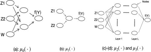
Here, $f(x)=\max (x,0)$ is the ReLU activate function, and $A_1=(\begin{array}{ccc}{a}_{11}^{(1)}& a_{12}^{(1)}& a_{13}^{(1)}\\ a_{21}^{(1)}& a_{22}^{(1)}& a_{23}^{(1)}\end{array})$ and $A_2=(a_1^{(2)},a_2^{(2)})$ are the model parameters. Corresponding to (3), the true model parameter values are $a_{11}^{(1)}=a_{12}^{(1)}=a_{23}^{(1)}=1,a_{13}^{(1)}=a_{21}^{(1)}=a_{22}^{(1)}=0$ and $(a_1^{(2)},a_2^{(2)})=(1,-1)$. In our analysis, we assume that we know the model form (4) but do not know the values of model parameters A₁ and A₂.

For the testing data, we consider two scenarios: (i) [IID case] ${\mathbf{x}}_{\mathrm{ }\text{new}}\stackrel{\mathrm{ }\text{iid}}{\sim }N({\mu }_x,{\Sigma }_x)$ and, given ${\mathbf{x}}_{\mathrm{ }\text{new}},({\mathbf{x}}_{\mathrm{ }\text{new}},y_{\mathrm{ }\text{new}})$ follows (3); (ii) [Non-IID case] the marginal distribution ${\mathbf{x}}_{\mathrm{ }\text{new}}\stackrel{\mathrm{ }\text{iid}}{\sim }(T_1,T_2,T_3)$ and, given ${\mathbf{x}}_{\mathrm{ }\text{new}},({\mathbf{x}}_{\mathrm{ }\text{new}},y_{\mathrm{ }\text{new}})$ follows (3). Here, $T_1,T_2,T_3$ are iid random variables from the t-distribution with degrees of freedom 3 and non-centrality parameter 1.

In addition to (a) the true model ${\mu }_0(·)$, four wrong learning models are considered:$$\begin{array}{c}\text{(b)}\hspace{1em}{\mu }_1({\mathbf{x}}_i)=f(B{\mathbf{z}}_i)\hspace{1em}(\mathrm{ }\text{partially}\mathrm{ }\text{correct}\mathrm{ }\text{neural}\mathrm{ }\text{network}\\ \text{model},\mathrm{ }\text{missing}\mathrm{ }{w}_i);\end{array}$$$$\begin{array}{c}\text{(c)}\hspace{1em}{\mu }_2({\mathbf{x}}_i)=f(C_{20}f(C_{19}\cdots f(C_1\mathbf{x})))\\ \mathrm{\hspace{1em}}\mathrm{\hspace{1em}}(\mathrm{ }\text{deep}\mathrm{ }\text{neural}\text{network}\mathrm{ }\text{model}\mathrm{ }\text{with}\mathrm{ }20\mathrm{ }\text{layers});\end{array}$$$$\begin{array}{c}\text{(d)}\hspace{1em}{\mu }_3({\mathbf{x}}_i)=f(D_{100}f(D_{99}\cdots f(D_1\mathbf{x})))\\ \text{\hspace{1em}\hspace{1em} (}\text{deep}\mathrm{ }\text{neural}\text{network}\mathrm{ }\text{model}\mathrm{ }\text{with}\mathrm{ }100\mathrm{ }\text{layers});\end{array}$$$$\text{(e)}\hspace{1em}{\mu }_4({\mathbf{x}}_i)={\eta }_0\mathrm{\hspace{1em}}\mathrm{\hspace{1em}}(\mathrm{ }\text{without}\mathrm{ }\text{any}\mathrm{ }\text{covariates}\mathrm{ }),$$where ${\mathbf{z}}_i={(z_{i1},z_{i2})}^T,B=(b_1,b_2),C_1,D_1\in {\mathbb{R}}^{20\times 3},C_{20},D_{100}\in {\mathbb{R}}^{1\times 20}$, and $C_i,D_j\in {\mathbb{R}}^{20\times 20},2\le i\le 19,2\le j\le 99$. In our analysis, the neural network models ${\mu }_0(·)$ - ${\mu }_3(·)$ are fit using the neuralnet package (cran.r-project.org/web/packages/neuralnet/).

The Neuralnet package is an off-the-shelf machine learning algorithm. Its emphasis is on learning and not on model parameter estimation. Even under the true model ${\mu }_0(·)$, the estimates of model parameters from Neuralnet are not very accurate (see Table 1). In the table, “Opt-MSE” refers to a code that we wrote by directly minimizing $\mathrm{ }\text{MSE}={\sum }_{j=1}^n{(y_j-{\mu }_0({\mathbf{x}}_j))}^2$, which can be implemented when the neural network is small. The calculation in the table is based on 20 repeated runs, each with a training dataset of size n = 300 from model (3).

Table 1 Mean square error of each parameter in μ₀ (training data n = 300; repetition = 10).

MSE	a11	a12	a13	a21	a22	a23	b1	b2
Opt-MSE	0.07	0.059	0.31	0.154	0.109	0.124	0.06	0.101
Neuralnet	4.87	5.9	1.53	1.14	2.23	2.08	4.87	0.84

Reported in Table 2 are the coverage rate and average interval length of predictive intervals computed under 10 = 5 × 2 settings with five different learning models ${\mu }_k(·),k=0,1,\dots ,4$, and in two scenarios. The analysis is repeated for 10 times with 10 simulated training datasets from model (3). We use 10 repetitions and not a greater number, because it takes a long time to fit a neural network model. However, for each of the 10 training datasets, 20 pairs of $(y_{\mathrm{ }\text{new}},{\mathbf{x}}_{\mathrm{ }\text{new}})$ are used. So, for the reported values, each is computed using 10 × 20 = 200 pairs of $(y_{\mathrm{ }\text{new}},{\mathbf{x}}_{\mathrm{ }\text{new}})$. For the true neural network model ${\mu }_0(·)$, Opt-MSE is also used to fit the model. As we can see in Table 2, under the IID scenario, all predictive intervals are valid with a correct coverage. The best one with the shortest interval length is the one that uses the correct model and Opt-MSE estimation method. In the non-IID case, only the shallow neural network models provide valid predictions, and among them, Opt-MSE can give us confidence intervals with half the width. Indeed, when a wrong learning model is used, the IID assumption is essential for the prediction validity and the use of a wrong model often results in wider intervals. Furthermore, the estimation of model parameters seems to also have a big impact on prediction.

Table 2 Performance of 95% predictive intervals under five different learning models and in two scenarios: coverage rates (before brackets) and average interval lengths (inside brackets) (training data size = 300; testing data size = 20; repetition = 10).

	True model		Wrong model
	${\mu }_0(·)$		${\mu }_1(·)$	${\mu }_2(·)$	${\mu }_3(·)$	${\mu }_4(·)$
	Opt-MSE	Neuralnet	Nueralnet	Nueralnet	Nueralnet	Nueralnet
IID scenario	0.995 (4.462)	0.99 (4.608)	0.99 (4.809)	0.99 (5.212)	0.99 (5.201)	0.985 (5.26)
Non-IID scenario	0.955 (4.52)	0.985 (9.327)	0.98 (9.77)	0.71 (5.899)	0.695 (5.201)	0.685 (5.277)

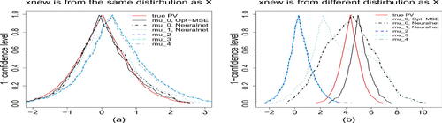
To get a full picture of the predictive intervals at all levels, we plot in Figure 2 the predictive curves of $y_{\mathrm{ }\text{new}}$. The plots are based on the first training dataset and making prediction for (a) the IID case with the realization ${\mathbf{x}}_{\mathrm{ }\text{new}}=(-0.909,-1.149,-0.771)$, and (b) the non-IID case with the realization ${\mathbf{x}}_{\mathrm{ }\text{new}}=(3.653,1.748,1.063)$. The realized value of ${\mu }_0({\mathbf{x}}_{\mathrm{ }\text{new}})$ is 0 and 4.338 in (a) and (b), respectively. From Figure 2, we see that the use of a wrong model ${\mu }_1(·)$–${\mu }_4(·)$ results in wider predictive curve (and predictive intervals at all levels $1-\alpha \in (0,1)$) in both IID and non-IID cases. Although the shallow neural network models ${\mu }_0(·)$ and ${\mu }_1(·)$ can provide good coverage rates, the predictive curves in the non-IID case are much wider than other approaches. This peculiar phenomenon occurs even when we assume to know the true model structure ${\mu }_0(·)$, indicating the importance of estimating model parameters accurately. Furthermore, in the non-IID case, there are large shifts when we use deep neural network models ${\mu }_2(·)$ and ${\mu }_3(·)$, leading to invalid predictions. The best prediction result is from the one obtained by using the correct learning model ${\mu }_0(·)$ with the more accurate parameter estimation method Opt-MSE. The message is the same as what we have learned from Table 2, which also exactly mirrors what is found in the case study of linear models in Xie and Zheng (2020).

Fig. 2 Plots of predictive curves for (a) ${\mathbf{x}}_{\mathrm{ }\text{new}}\stackrel{\mathrm{ }\text{iid}}{\sim }{\mathbf{x}}_i$ and (b) ${\mathbf{x}}_{\mathrm{ }\text{new}}\cancel{\sim }{\mathbf{x}}_i$. In each plot, the red solid curve is the target (oracle) predictive curve ${\mathrm{ }\text{PV}}_n(y)=2\max \{\Phi (y-{\mu }_{\mathrm{ }\text{new}}),1-\Phi (y-{\mu }_{\mathrm{ }\text{new}})\}$, obtained assuming that the distribution of $y_{\mathrm{ }\text{new}}\sim N({\mu }_{\mathrm{ }\text{new}},1)$ is completely known. The two predictive curves obtained using ${\mu }_0(·)$ are in black (solid line for Opt-MSE; dashed line for Neuralnet). The other predictive curves (all in a dashed or broken line and in various colors) are obtained using the other four wrong working models.

4 Conclusion

Professor Efron pointed out that “the 21st Century has seen the rise of a new breed of what can be called ‘pure prediction algorithms’.” We are fully in agreement with Professor Efron’s discussion that the prediction algorithms “can be stunningly successful,” and that “the emperor has nice clothes but they’re not suitable for every occasion.” Along the same line and under the setting of conformal prediction, we have demonstrated and explained how and why a prediction method can be successful under the IID assumption, even if the learning model is completely wrong. More importantly, we have also demonstrated that it is still meaningful, and often crucial, to build our prediction algorithms based on a good practice of modeling, estimation and inference. We fully anticipate and believe that “the most powerful ideas of Twentieth Century statistics”—modeling, estimation, and inference, will play a pivotal role in building the mathematical foundation of modern data science and in fully realizing its potential for real-world applications.

Funding

The research is supported in part by research grants from NSF.

References

- Barber, R. F., Candes, E. J., Ramdas, A., and Tibshirani, R. J. (2019a), “The Limits of Distribution-Free Conditional Predictive Inference,” arXiv no. 1903.04684.
- ——— (2019b), “Predictive Inference With the Jackknife+,” arXiv no. 1905.02928.
- Efron, B. (1998), “R. A. Fisher in the 21st Century (Invited paper Presented at the 1996 R. A. Fisher Lecture),” Statistical Science, 13, 95–122. DOI: 10.1214/ss/1028905930.
- Lei, J., G’Sell, M., Rinaldo, A., Tibshirani, R. J., and Wasserman, L. (2018), “Distribution-Free Predictive Inference for Regression,” Journal of the American Statistical Association, 113, 1094–1111. DOI: 10.1080/01621459.2017.1307116.
- Shafer, G., and Vovk, V. (2008), “A Tutorial on Conformal Prediction,” Journal of Machine Learning Research, 9, 371–421.
- Shen, J., Liu, R., and Xie, M. (2018), “Prediction With Confidence—A General Framework for Predictive Inference,” Journal of Statistical Planning and Inference, 195, 126–140. DOI: 10.1016/j.jspi.2017.09.012.
- Singh, K., Xie, M., and Strawderman, W. E. (2005), “Combining Information From Independent Sources Through Confidence Distributions,” The Annals of Statistics, 33, 159–183. DOI: 10.1214/009053604000001084.
- Vovk, V., Gammerman, A., and Shafer, G. (2005), Algorithmic Learning in a Random World, New York: Springer.
- Vovk, V., Shen, J., Manokhin, V., and Xie, M. (2019), “Nonparametric Predictive Distributions by Conformal Prediction,” Machine Learning, 108, 445–474. DOI: 10.1007/s10994-018-5755-8.
- Xie, M., and Singh, K. (2013), “Confidence Distribution, the Frequentist Distribution Estimator of a Parameter” (with discussion), International Statistical Review, 81, 3–39. DOI: 10.1111/insr.12000.
- Xie, M., and Zheng, Z. (2020), “Homeostasis Phenomenon in Predictive Inference When Using a Wrong Learning Model: A Tale of Random Split of Data Into Training and Test Sets,” arXiv no. 2003.08989.