Variable Selection in the Presence of Factors: A Model Selection Perspective

Abstract

In the context of a Gaussian multiple regression model, we address the problem of variable selection when in the list of potential predictors there are factors, that is, categorical variables. We adopt a model selection perspective, that is, we approach the problem by constructing a class of models, each corresponding to a particular selection of active variables. The methodology is Bayesian and proceeds by computing the posterior probability of each of these models. We highlight the fact that the set of competing models depends on the dummy variable representation of the factors, an issue already documented by Fernández et al. in a particular example but that has not received any attention since then. We construct methodology that circumvents this problem and that presents very competitive frequentist behavior when compared with recently proposed techniques. Additionally, it is fully automatic, in that it does not require the specification of any tuning parameters.

Keywords:

• Bayes factor
• Categorical variables
• Multiplicity
• Objective methods
• Prior distributions
• Variable selection

1 Introduction

Consider a Gaussian multiple regression problem where the set of potential explanatory variables is composed of $x_1,\dots ,x_k$ (numerical variables) and factors (categorical variables) ${\Lambda }_1,\dots ,{\Lambda }_p$, each with a number of levels denoted by ${\mathcal{l}}_1,\dots ,{\mathcal{l}}_p$ such that ${\mathcal{l}}_j\ge 2,$ $j=1,\dots ,p$; let $L={\sum }_{j=1}^p{\mathcal{l}}_j$. Denote by $\mathit{y}={(y_1,\dots ,y_n)}^{\top }$ the vector of observations of the response variable.

The regression model that includes all the potential explanatory variables, also known as the full model, could initially be written as(1) $$\mathit{y}=\mathit{1}{\beta }_0+\mathit{X\alpha }+\mathit{Z\beta }+\mathit{\epsilon },$$(1) where $\mathit{X}$ is an n × k matrix, where line i contains the values of the numerical variables for the ith observation, and $\mathit{Z}=[{\mathit{Z}}_1|\cdots \left|{\mathit{Z}}_j\right|\cdots |{\mathit{Z}}_p]$ is an n × L matrix, where ${\mathit{Z}}_j=(z_{ir}^{(j)})$ is an $n\times {\mathcal{l}}_j$ matrix, with $z_{ir}^{(j)}=1$ if the ith observation takes on the rth level of Λ_j , and 0 otherwise, $i=1,\dots ,n,r=1,\dots ,{\mathcal{l}}_j,j=1,\dots ,p$. The $z_{·r}^{(j)}$ are called artificial or dummy variables. The parameter vectors are ${\mathit{\beta }}^{\top }=({\mathit{\beta }}_1^{\top },\dots ,{\mathit{\beta }}_p^{\top })$, with ${\mathit{\beta }}_j={({\beta }_{j1},\dots ,{\beta }_{j{\mathcal{l}}_j})}^{\top },j=1,\dots ,p$, and $\mathit{\alpha }={({\alpha }_1,\dots ,{\alpha }_k)}^{\top }$, whereas $\mathit{\epsilon }={({\epsilon }_1,\dots ,{\epsilon }_n)}^{\top }$ is the vector of residual variables, satisfying $\mathit{\epsilon }\sim \mathbf{N}(0,{\sigma }^2\mathit{I})$, with $\mathit{I}$ representing the identity matrix of order n and $\sigma >0$.

It is well-known that such model is not estimable: the design matrix $[\mathit{1}|\mathit{X}|\mathit{Z}]$ is not full-column rank, and hence the maximum likelihood equation does not have a unique solution; the model is overparameterized. The solution is typically to impose a full-rank reparameterization on this model. A popular choice is the so-called treatment parameterization, whereby for each factor Λ_j we choose a reference level, say r(j), and the effect on the mean value of the response for all other levels, ceteris paribus, is measured as an increment from the selected reference. In the notation above, this is equivalent to setting ${\beta }_{j,r(j)}=0$ and removing the r(j)th column from ${\mathit{Z}}_j$. We will later warn about the pitfalls of performing variable selection once we impose a full-rank reparameterization.

The variable selection problem in this context can be broadly defined as determining which potential regressors are relevant to explain the response. There is a very rich literature on this topic, which we briefly review in Section 2. Variable selection methods can be classified depending on whether (i) one considers all possible models defined by which subset of variables is relevant or (ii) only the model containing all variables (the full model) is considered. The difference exists in the two main inferential paradigms. See, for instance, Desboulets (2018) in the realm of frequentist methods and Castillo, Schmidt-Hieber, and Van Der Vaart (2015) for a Bayesian perspective. Both references use similar terminology: methods in (i) are “model selection” while those in (ii) correspond to “(point) estimation methods.” In this article, we also use this terminology.

We propose novel methodology to answer the variable selection problem from a model selection perspective. It is specifically tailored to the situation described above: there are both numerical variables and factors in the list of potential explanatory variables. The methodology is Bayesian and the selection among the class of competing models is based on the posterior probability of each of the models.

It is important to precisely state the notion of a factor being relevant, or active, that is present throughout this article. A numerical variable x_j is active if the associated coefficient, α_j , differs from zero. A factor Λ_j is declared active if at least one of the coefficients, β_jr , $r=1,\dots ,{\mathcal{l}}_j$, associated to its levels differs from zero. As we will indicate in Section 2, other articles only consider that a factor is present in a model if all its levels are included. We argue that this is not always the best approach, for several reasons. There is often some arbitrariness in constructing the levels of a factor, a typical example being when the factor results from discretizing a numerical variable. Because of the trade-off between complexity and fit, the relevance of a factor may be artificially downplayed by increasing its granularity. For this same reason, a factor can be deemed irrelevant just because the number of active levels is small relative to its dimension. Hence, one has to consider the models that include every combination of possible active levels for each factor.

In the context of an applied research about modeling of catch in a fishery, Fernández, Ley, and Steel (2002) is an example of declaring a factor active if at least one of its levels has a coefficient that differs from zero. They pointed out that, if one imposes a treatment parameterization to obtain a full-rank design matrix, then not all combinations of active levels will be achievable. We investigated this phenomenon in general and have concluded that if one follows the common practice of generating the class of competing models by removing columns of the design matrix after having selected a full-rank parameterization for the full model, the resulting class of models will not be exhaustive. Moreover, the missing models are parameterization-dependent.

To the best of our knowledge, this issue has not received any attention since Fernández, Ley, and Steel (2002). Hence, it is very likely that practitioners have been feeding variable selection packages with the full-rank design matrix and performing variable selection with factors unaware of the fact that some potentially important models were a priori excluded from the class of competing models. We offer a very general and systematic solution to this problem: generate the class of models by deleting columns from the overparameterized representation of the full model, stated in (1). The class thus generated is exhaustive but will unfortunately contain repeated models. We deal with this issue by keeping only one of each set of repeated models, excluding all the others from the analysis. This is formalized at the beginning of Section 3. In Section S.1 of the supplementary materials, we explore this phenomenon in the context of a model with only one factor with three levels.

Posterior model probabilities can be written as a function of the Bayes factor, which in turn require the specification of a prior distribution for the model-specific parameters. From a computational perspective, a prior that results in a marginal distribution for the data that is easy to compute is certainly advantageous, and this includes any of the so-called conventional priors (Berger and Pericchi 2001). Among these, our recommended choice is the robust prior of Bayarri et al. (2012), which is the one we use in the numerical results. This prior satisfies a number of attractive theoretical properties and results in a closed-form Bayes factor. We also consider approximations to the Bayes factor obtained via selection criteria like Akaike information criterion (AIC proposed by Akaike (1974)) or the Bayesian information criterion (BIC proposed by Schwarz (1978)). All the details regarding the calculations involved in obtaining and exploring the posterior distribution on the model space are described in Section 3.1.

A major contribution of this article concerns the prior over the model space. The problem with factors turns out to be more delicate than expected. We show that direct extensions of the standard objective priors (like the constant prior used by Fernández, Ley, and Steel 2002) lead to marginal inclusion probabilities that strongly depend on the number of levels of the factors. We conclude that the prior should be assigned hierarchically, in two levels, and propose a new prior distribution that generalizes Scott and Berger (2010) and that, among other properties, accounts for the multiplicity issue concerning the number of predictors. Our proposal is put forth in Section 3.2.

In Section 4, we carry out a simulation study designed to compare the frequentist behavior of our methodology with alternative approaches. The results are very favorable to our proposal, especially if ones takes into consideration the fact that our method is fully automatic, in that it does not require the specification of any tuning parameters, and this makes it considerably easier to use.

When dealing with factors, one may be interested in deciding whether some of the levels can be merged or grouped. Once we obtain the posterior distribution over the model space, we devise a strategy to address this issue that only requires the specification of a credibility level (in the simulations, we set it at 95%). This is the subject of Section 5.

2 Literature Review

As highlighted in the previous section, variable selection methods are either model-selection based or estimation-based. Estimation techniques are usually seen as computationally more appealing (since only one model is fitted) while the results in model selection approaches are arguably richer, allowing for example to produce model averaged estimates and predictions (see Steel 2020 for a recent and complete revision of model averaging methods). With respect to the main theoretical challenges, the implementation of model selection methods requires careful handling of the issue of multiplicity. In estimation methods, the main difficulty is how to properly induce sparsity, since some of the parameters are to be encouraged to be zero.

Multiplicity comes from the fact that models of similar complexity are going to be compared. If the number of models of similar complexity is large, it is possible that just by chance one of those models will be deemed significant when in fact it is not. Scott and Berger (2010) studied ways of multiplicity control from the Bayesian perspective.

On the other hand, sparsity must be induced in estimation methods, given that the assumed (full) model often contains many variables whose impact on the response is doubtful and a strong reduction in dimensionality is sought. Depending on the statistical paradigm, this is normally achieved either by regularization methods or by priors on the regression parameters that have a substantial mass in the neighborhood of zero (see below for references).

Obviously, estimation methods are not exposed to multiplicity issues and one can argue that model selection techniques automatically induce sparsity—because all the simpler models are taken into account and these are indirectly favored by penalizations over the complexity (e.g., AIC, BIC, Bayes factors, etc.)

The variable selection problem with factors (generally embedded in a context of how to treat grouped variables) has been approached from the two perspectives mentioned above. In all cases, a factor is introduced using a group of dummy variables.

With respect to estimation methods, one of the first attempts to include factors is Yian and Lin (2006) (from a frequentist perspective); they developed extensions of regularization methods (e.g., the group lasso). This technique has the characteristic of handling dummy variables for a factor in block (either all or none are included). Raman et al. (2009) proposed the Bayesian version of Yian and Lin (2006), introducing the Bayesian group-LASSO method. Farcomeni (2010) is a similar implementation but based on the continuous spike and slab priors introduced by George and McCulloch (1993). Later, Friedman, Hastie, and Tibshirani (2010) argued that the group lasso does not yield sparsity within a group since “if a group of parameters is nonzero, they will all be nonzero” and proposes a penalty that yields sparsity at both the group and individual feature levels. More recently, in a related but different context than variable selection, Pauger and Wagner (2019) have focused on the idea of developing priors that allow different levels of factors to fuse, as an alternative procedure to obtain sparse results. In the context of ANOVA models, Bondell and Reich (2009) is an earlier reference proposing methodology to simultaneously determine which factors are active and to detect relevant differences among levels of active factors. Their method is called CASANOVA (for collapsing and shrinkage in ANOVA) and is based on constrained regression.

Concerning model selection methods, Clyde and Parmigiani (1998) and Fernández, Ley, and Steel (2002) described real applications of variable selection with factors where dummy variables coding a factor are not treated in blocks. The Bayesian Sparse Group Selection by Chen et al. (2016) and the accompanying R-package (Lee and Chen 2015) is an implementation of the spike and slab priors that considers not only the factors as variables to select from but also the levels within each factors. Nevertheless, none of these authors discuss the issue of multiplicity. Finally, Chipman (1996) is an early reference that warns about the necessity of controlling for multiplicity within the group of dummy variables defining a factor.

3 Variable Selection With Factors: Our Proposal

Consider the problem described in Section 1. If one adopts a full-rank parameterization of (1) and generates the class of competing models by deleting columns of the resulting design matrix, the set of entertained models will not be exhaustive. Results can be highly affected if important models are lost.

To overcome this fact, we propose, following on Fernández, Ley, and Steel (2002), to start from the overparameterized model (1) and delete columns of the matrix $[\mathit{X}|\mathit{Z}]$ to generate the model space. We formally obtain a total of $2^{k+L}$ models, but some of these are repeated, they are reparameterizations of each other. Precisely, these models are those that, for a given factor with $\mathcal{l}$ levels, contain either $\mathcal{l}-1$ or $\mathcal{l}$ dummies—and we want to keep only one of them. In what follows, we denote by $\mathcal{M}$ the set containing only the models obtained using this process, that is, $\mathcal{M}$ is the set of unique models generated by deleting columns of the matrix $[\mathit{X}|\mathit{Z}]$. Among the repeated models, the convention we follow is to retain only the overparameterized model (the one with $\mathcal{l}$ dummies); this one will act as the representative of the corresponding set of repeated models. We will see in Section 3.1 that it is irrelevant from a model selection perspective which model we choose as the representative.

We refer again to Section S.1 of the supplementary materials for a better comprehension of this phenomenon. Note that, as a reviewer pointed out, there may be situations where a particular full-rank parameterization is chosen because it is meaningful in the context of the application. As a consequence, it may be the case that the resulting excluded models are implausible a priori, in which case the impact of the restriction may not be very important. For models with several predictors, this may be difficult to assess.

Any model in $\mathcal{M}$ can be identified with a parameter vector $(\mathit{\gamma },\mathit{\delta })\in {\{0,1\}}^{k+L}$, where ${\mathit{\gamma }}^{\top }=({\gamma }_1,\dots ,{\gamma }_k)$, ${\mathit{\delta }}^{\top }=({\mathit{\delta }}_1^{\top },\dots ,{\mathit{\delta }}_p^{\top }),{\mathit{\delta }}_j^{\top }=({\delta }_{j1},\dots ,{\delta }_{j{\mathcal{l}}_j})$, and ${\gamma }_i=1$ if x_i is in the model (0 otherwise) and ${\delta }_{jr}=1$ if level r of factor Λ_j is in the model (0 otherwise), $i=1,\dots ,k,r=1,\dots ,{\mathcal{l}}_j,j=1,\dots ,p$. Stating that a variable is in a model is the same as saying that the corresponding column of $\mathit{X}$ was not deleted; likewise, level r of factor Λ_j is in the model if the corresponding column of ${\mathit{Z}}_j$ was not deleted. We will refer to a particular model interchangeably by either $M_{\mathit{\gamma },\mathit{\delta }}$ or simply $(\mathit{\gamma },\mathit{\delta })$. As an example, in the case of a problem with a single factor with $\mathcal{l}=3$ levels and no numerical variables, we would have: $\mathcal{M}=\{M_{(0,0,0)},M_{(1,0,0)},M_{(0,0,1)},M_{(0,1,0)},M_{(1,1,1)}\}$.

The cardinality of $\mathcal{M}$ and the fact that it contains only unique models are explicitly stated in the next result.

Theorem 1.

Suppose the rank of $[\mathit{1}|\mathit{X}|\mathit{Z}]$ in (1) is $1+k+L-p$, and $n\ge 1+k+L-p$, then $\mathcal{M}$ is composed only of unique models (no model is repeated). Furthermore:(2) $$\#\mathcal{M}=2^k\times \prod _{j=1}^p(2^{{\mathcal{l}}_j}-{\mathcal{l}}_j).$$(2)

Proof.

See the supplementary materials, Section S.3. □

A full-rank parameterization of the full model produces a model space with $2^k{\prod }_{j=1}^p{2}^{{\mathcal{l}}_j-1}$ models, so that the number of models that disappears is, according to Theorem 1,$$2^k\left[\prod _{j=1}^p(2^{{\mathcal{l}}_j}-{\mathcal{l}}_j)-\prod _{j=1}^p{2}^{{\mathcal{l}}_j-1}\right].$$

If, as in the example above, k = 0, p = 1, and $\mathcal{l}=3$, then $\#\mathcal{M}=5$, and only one model would have disappeared in a full-rank parameterization. However, if k = 3 and p = 3, with ${\mathcal{l}}_1=3,{\mathcal{l}}_2=4$, and ${\mathcal{l}}_3=4$, we have $\#\mathcal{M}=5760,$ of which, if we were to choose a full-rank parameterization, 3712 models would disappear (more than 60%).

The goal now is to produce the posterior distribution over $\mathcal{M}$, which we denote by $f(\mathit{\gamma },\mathit{\delta }|\mathit{y})$. This is the subject of the remainder of this section: in Section 3.1 we present the details concerning the calculation of $f(\mathit{\gamma },\mathit{\delta }|\mathit{y})$, and Section 3.2 is devoted to the very important issue of specifying the prior distribution over $\mathcal{M}$, which we denote by $f(\mathit{\gamma },\mathit{\delta })$. The reason why we first describe the posterior is because the process of evaluating the characteristics of the prior selections will involve investigating their impact on the posterior.

Before we proceed, let us introduce some extra notation. A useful function of $(\mathit{\gamma },\mathit{\delta })$ is the one that indicates which factors are active in a particular model: $\mathit{\tau }=\mathit{\tau }(\mathit{\delta })={({\tau }_1,\dots ,{\tau }_p)}^{\top }$, where ${\tau }_j={\tau }_j({\mathit{\delta }}_j)=1$ if ${\mathit{1}}^{\top }{\mathit{\delta }}_j\ge 1$ (0 otherwise), $j=1,\dots ,p$. To clarify the notation, in Table S.4 of Section S.2 of the supplementary materials we have provided the values for the vectors $\mathit{\gamma },\mathit{\delta }$ and $\mathit{\tau }$ for all the models spanned as we delete columns from $[\mathit{X}|\mathit{Z}]$ in (1) of a problem with one covariate (k = 1) and two factors (p = 2) with ${\mathcal{l}}_1=2$ and ${\mathcal{l}}_2=3$. We also indicate whether each model is a member of $\mathcal{M}$.

The posterior inclusion probability of factor Λ_j (sum of the posterior probabilities of models with at least one of its levels included) can be compactly expressed as $p({\tau }_j=1|\mathit{y})$; the posterior inclusion probability of a covariate x_i is $p({\gamma }_i=1|\mathit{y})$. Formally,(3) $$\begin{array}{c}p({\gamma }_i=1|\mathit{y})=\sum _{\mathit{\gamma },\mathit{\delta }:{\gamma }_i=1}f(\mathit{\gamma },\mathit{\delta }|\mathit{y}),\\ p({\tau }_j=1|\mathit{y})=\sum _{\mathit{\gamma },\mathit{\delta }:{\tau }_j=1}f(\mathit{\gamma },\mathit{\delta }|\mathit{y}).\end{array}$$(3)

The corresponding prior probabilities are obtained by replacing in the formulas above $f(\mathit{\gamma },\mathit{\delta }|\mathit{y})$ with $f(\mathit{\gamma },\mathit{\delta })$.

3.1 Posterior Distribution

The posterior probabilities of each of the competing models can be expressed as(4) $$f(\mathit{\gamma },\mathit{\delta }|\mathit{y})\propto m_{\mathit{\gamma },\mathit{\delta }}(\mathit{y})f(\mathit{\gamma },\mathit{\delta }),$$(4) where $m_{\mathit{\gamma },\mathit{\delta }}(\mathit{y})$ is the prior predictive density of the data under this model:$$\begin{array}{c}{m}_{\mathit{\gamma },\mathit{\delta }}(\mathit{y})=\int \mathrm{N}(\mathit{y}|\mathit{1}{\beta }_0+{\mathit{X}}_{\mathit{\gamma }}{\mathit{\alpha }}_{\mathit{\gamma }}+{\mathit{Z}}_{\mathit{\delta }}{\mathit{\beta }}_{\mathit{\delta }},{\sigma }^2\mathit{I})\\ \hspace{1em}\pi ({\beta }_0,{\mathit{\alpha }}_{\mathit{\gamma }},{\mathit{\beta }}_{\mathit{\delta }},\sigma )d{\beta }_{0}d{\mathit{\alpha }}_{\mathit{\gamma }}d{\mathit{\beta }}_{\mathit{\delta }}d\sigma ,\end{array}$$ with $\pi ({\beta }_0,{\mathit{\alpha }}_{\mathit{\gamma }},{\mathit{\beta }}_{\mathit{\delta }},\sigma )$ denoting the prior distribution on the model-specific parameters. The matrices ${\mathit{X}}_{\mathit{\gamma }}$ and ${\mathit{Z}}_{\mathit{\delta }}$ result from selecting the corresponding columns in $\mathit{X}$ and $\mathit{Z}$ (and similarly for ${\mathit{\alpha }}_{\mathit{\gamma }}$ and ${\mathit{\beta }}_{\mathit{\gamma }}$). Alternatively, we can rewrite (4) as $f(\mathit{\gamma },\mathit{\delta }|\mathit{y})\propto B_{\mathit{\gamma },\mathit{\delta }}f(\mathit{\gamma },\mathit{\delta })$, where $B_{\mathit{\gamma },\mathit{\delta }}=m_{\mathit{\gamma },\mathit{\delta }}(\mathit{y})/m_{\mathit{0},\mathit{0}}(\mathit{y})$ is the so-called Bayes factor of model $M_{\mathit{\gamma },\mathit{\delta }}$ to the null model.

The choice of $\pi ({\beta }_0,{\mathit{\alpha }}_{\mathit{\gamma }},{\mathit{\beta }}_{\mathit{\delta }},\sigma )$ from an objective point of view has been an important research question since at least Zellner and Siow (1980); see Liang et al. (2008) and Bayarri et al. (2012) for in-depth reviews. A substantial part of the literature has focused on priors that have the peculiarity of using a mixture of normal densities for $({\mathit{\alpha }}_{\mathit{\gamma }},{\mathit{\beta }}_{\mathit{\delta }})$, centered at zero and with a variance proportional to the information matrix, and standard noninformative priors for the common parameters β₀ and σ. This approach was named conventional by Berger and Pericchi (2001) and Bayarri and García-Donato (2007), a term that we also adopt. Conventional priors have been successfully implemented by many authors, like Fernández, Ley, and Steel (2001) and Liang et al. (2008). Recently, Bayarri et al. (2012) have shown that this class of priors satisfies a number of desirable properties including several types of invariance, predictive matching and consistency.

For any conventional prior, we have that the expression for the corresponding Bayes factor is(5) $$B_{\mathit{\gamma },\mathit{\delta }}=\mathcal{I}\left(\frac{{\text{SSE}}_{\mathit{\gamma },\mathit{\delta }}}{{\text{SSE}}_{\mathit{0},\mathit{0}}},1,\kappa (\mathit{\gamma },\mathit{\delta })+1\right),$$(5) where $\kappa (\mathit{\gamma },\mathit{\delta })+1$ is the rank of the matrix $[\mathit{1}|{\mathit{X}}_{\mathit{\gamma }}|{\mathit{Z}}_{\mathit{\delta }}]$, $\text{SSE}$ stands for the sum of squared errors and $\mathcal{I}$ is obtained by computing a one-dimensional integral:(6) $$\mathcal{I}(q,{\kappa }_0,{\kappa }_1)=\int {(1+q g)}^{-(n-{\kappa }_0)/2} {(1+g)}^{(n-{\kappa }_1)/2} h(g)dg;$$(6) where h is the mixing density that gives rise to the different conventional priors proposed in the literature. Our recommended choice is the robust prior in Bayarri et al. (2012) that corresponds to(7) $$\begin{array}{c}h(g)=\frac{1}{2}{\left(\frac{1+n}{\kappa (\mathit{\gamma },\mathit{\delta })+1}\right)}^{1/2}{(g+1)}^{-3/2},\\ g>\frac{n+1}{\kappa (\mathit{\gamma },\mathit{\delta })+1}-1.\end{array}$$(7)

Formula (5) was derived in Bayarri and García-Donato (2007), and is valid regardless of whether $[\mathit{1}|{\mathit{X}}_{\mathit{\gamma }}|{\mathit{Z}}_{\mathit{\delta }}]$ is full-rank or not. This result justifies the fact that it is irrelevant which element of the set of repeated models that are reparameterizations of each other is chosen as its representative: note that (5) only depends on the rank of the design matrix and on the sum of squared errors, and these are both invariant under reparameterizations. In what follows, we refer to $\kappa (\mathit{\gamma },\mathit{\delta })$ as the “dimension” of the model (any model in $\mathcal{M}$ can be reparameterized as a linear model with full-rank design matrix with $\kappa (\mathit{\gamma },\mathit{\delta })$ columns apart from the intercept). We again refer to Table S.4 of Section S.2 of the supplementary materials to clarify the interpretation of $\kappa (\mathit{\gamma },\mathit{\delta })$ in an example. An explicit expression for $\kappa (\mathit{\gamma },\mathit{\delta })$ and related results are described in the supplementary materials, Section S.4 (in particular, in Result S.1).

Model selection criteria like BIC and AIC are often used to approximate actual Bayes factors. We consider these approaches in our simulation experiments. To be precise,(8) $${\text{BIC}}_{\mathit{\gamma },\mathit{\delta }}=n\hspace{0.17em}\text{ln}\hspace{0.17em}({\text{SSE}}_{\mathit{\gamma },\mathit{\delta }}/n)+(\kappa (\mathit{\gamma },\mathit{\delta })+1)\hspace{0.17em}\text{ln}\hspace{0.17em}n$$(8) and(9) $${\text{AIC}}_{\mathit{\gamma },\mathit{\delta }}=n\hspace{0.17em}\text{ln}\hspace{0.17em}({\text{SSE}}_{\mathit{\gamma },\mathit{\delta }}/n)+2(\kappa (\mathit{\gamma },\mathit{\delta })+1)$$(9) and the approximations we will also implement result from using(10) $$B_{\mathit{\gamma },\mathit{\delta }}\approx \hspace{0.17em}\text{exp}\hspace{0.17em}\left[-({\mathrm{C}}_{\mathit{\gamma },\mathit{\delta }}-{\mathrm{C}}_{\mathit{0},\mathit{0}})/2)\right],$$(10) where ${\mathrm{C}}_{\mathit{\gamma },\mathit{\delta }}$ is given either by (8) or (9). Although arguably not fully Bayesian, there is some partial justification for this strategy, especially for the case of BIC, as it was originally developed as a general (asymptotic) approximation to the prior predictive distribution of the data, and hence to the Bayes factor.

3.2 Prior Distribution

We now turn to the prior model probabilities, $f(\mathit{\gamma },\mathit{\delta })$. Fernández, Ley, and Steel (2002), used the constant prior over the whole model space:(C) $$f(\mathit{\gamma },\mathit{\delta })={\left(\#\mathcal{M}\right)}^{-1}.$$(C)

Scott and Berger (2010) showed that it should be through the prior distribution over the model space that one should control for multiplicity. A main conclusion in their work is that, in variable selection, the constant prior does not provide such controlling effect and they instead advocate for the use of a prior inversely proportional to the number of models of a given dimension. Interestingly, related considerations about the model space led Chen and Chen (2008) to propose a generalization of BIC that outperforms standard BIC in problems with a very large number of covariates.

In our context, a direct implementation of Scott and Berger (2010) would translate into(SB) $$f(\mathit{\gamma },\mathit{\delta })={\left[{\mathcal{F}}_k^{{\mathcal{l}}_1,\dots ,{\mathcal{l}}_p}(\kappa (\mathit{\gamma },\mathit{\delta })) (L-p+k+1)\right]}^{-1},$$(SB) where ${\mathcal{F}}_k^{{\mathcal{l}}_1,\dots ,{\mathcal{l}}_p}(r)$ is the number of models in $\mathcal{M}$ which have dimension r in a problem with k numerical variables and p factors with number of levels ${\mathcal{l}}_1,\dots ,{\mathcal{l}}_p$; see Result S.1 in the supplementary materials, Section S.4.

Theorem S.1 in the supplementary materials, Section S.4 establishes that both (C) and (SB) violate the assumption, widely accepted in the literature, that the prior inclusion probabilities of variables should be 1/2, independently of the number of variables entertained. For example, in a problem with just one factor with four levels, the prior probability of the factor is 0.92 in the case of (C) and 0.75 with (SB), but with two factors with 8 and 4 levels, the prior probability of the factors is 0.99 and 0.77 with (C) and 0.87, 0.77 with (SB), respectively. Without factors, prior inclusion probabilities of variables are 1/2 for the great majority of default choices, including the constant and the beta-binomial (of which the Scott and Berger prior is a particular case).

The key to finding alternatives priors that respect this assumption is to introduce $\mathit{\tau }$ in the formulation, and to construct the prior in two stages. Begin by noticing that, because $\mathit{\tau }$ is a deterministic function of $\mathit{\delta }$, we have$$f(\mathit{\gamma },\mathit{\delta })=f(\mathit{\gamma },\mathit{\delta },\mathit{\tau })=f(\mathit{\delta }|\mathit{\gamma },\mathit{\tau }) f(\mathit{\gamma },\mathit{\tau }),\text{if}\mathrm{ }\mathit{\tau }=\mathit{\tau }(\mathit{\delta }).$$

Next, we discuss these two probability distributions.

3.2.1 About the Marginal $\mathit{\gamma },\mathit{\tau }$

Since the prior $f(\mathit{\gamma },\mathit{\tau })$ corresponds to the marginal for the parameters that indicate which variables and factors are active, as long as it distributes probabilities in a way that $p({\tau }_j=1)=p({\gamma }_i=1)=1/2$, we will have a prior over the model space with the required property. The obvious candidates for these two distributions are the constant and the Scott and Berger prior. The constant prior is(11) $$f(\mathit{\gamma },\mathit{\tau })=2^{-(k+p)}$$(11) while the Scott and Berger-type prior is(12) $$f(\mathit{\gamma },\mathit{\tau })={\left[(k+p+1)\left(\begin{array}{c}k+p\\ {\mathit{1}}^{\top }\mathit{\delta }+{\mathit{1}}^{\top }\mathit{\gamma }\end{array}\right)\right]}^{-1}.$$(12)

3.2.2 About the Conditional $\mathit{\delta }|\mathit{\gamma },\mathit{\tau }$

The function $f(\mathit{\delta }|\mathit{\gamma },\mathit{\tau })$ distributes the probability among the set of models that have a certain combination of active factors and variables (those corresponding to the ones in $\mathit{\gamma },\mathit{\tau }$). This set of models can be formally expressed as(13) $$\begin{array}{c}\mathcal{M}(\mathit{\gamma },\mathit{\tau })=\{(\mathit{\gamma },\mathit{\delta })\in \mathcal{M}: \mathit{\gamma }=\mathit{\gamma },\\ \hspace{1em}\min \{{\mathit{1}}^{\top }{\mathit{\delta }}_j,1\}={\tau }_j,j=1,\dots ,p\},\end{array}$$(13) giving rise to a partition of $\mathcal{M}$ into $2^{k+p}$ sets of models: $\left\{\mathcal{M}(\mathit{\gamma },\mathit{\tau }):(\mathit{\gamma },\mathit{\tau })\in {\{0,1\}}^{k+p}\right\}$. Explicit expressions for the cardinality of $\mathcal{M}(\mathit{\gamma },\mathit{\tau })$ and related results are collected in Result S.2 in the supplementary materials, Section S.4.

We are now able to define two possible objective priors for $\mathit{\delta }|\mathit{\gamma },\mathit{\tau }$. We can have a prior that is constant for all models in $\mathcal{M}(\mathit{\gamma },\mathit{\tau })$:(14) $$f(\mathit{\delta }|\mathit{\gamma },\mathit{\tau })={\left[\#\mathcal{M}(\mathit{\gamma },\mathit{\tau })\right]}^{-1}$$(14) or a prior that assigns probability inversely proportional to the number of models of the same dimension in $\mathcal{M}(\mathit{\gamma },\mathit{\tau })$:(15) $$\begin{array}{c}f(\mathit{\delta }|\mathit{\gamma },\mathit{\tau })=([{\mathcal{G}}^{{\mathcal{l}}_{j_1},\dots ,{\mathcal{l}}_{j_{m_2}}}(\kappa (\mathit{\gamma },\mathit{\delta })-{\mathit{1}}^{\top }\mathit{\gamma })]\\ \mathrm{\hspace{1em}}\mathrm{\hspace{1em}}[{\mathcal{l}}_{j_1}+\cdots +{\mathcal{l}}_{j_{m_2}}-2m_2+1]{)}^{-1},\end{array}$$(15) where, above, $(j_1,\dots ,j_{m_2})$ are the indices corresponding to the ones in $\mathit{\delta },m_2={\mathit{1}}^{\top }\mathit{\delta }$ and ${\mathcal{G}}^{{\mathcal{l}}_{j_1},\dots ,{\mathcal{l}}_{j_{m_2}}}(r)$ stands for the number of models in $\mathcal{M}(\mathit{\gamma },\mathit{\tau })$ with dimension r (cf. Result S.2 in the supplementary materials, Section S.4).

We then have four possibilities for $f(\mathit{\gamma },\mathit{\delta })$, corresponding to the different combinations, that we label CC for (11) and (14); CSB for (11) and (15); SBC for (12) and (14) and finally SBSB for (12) and (15). For all these, the prior inclusion probabilities of variables and factors are all 1/2, that is, $p({\tau }_j=1)=p({\gamma }_i)=1/2$.

3.2.3 Discriminating Between the Different Priors

To discriminate between the four possible prior choices, we start by investigating multiplicity control with respect to the inclusion of factors by performing the following experiment.

Experiment 1. We simulated data from the model (1) with n = 300 observations and p factors all with the same number of levels, ${\mathcal{l}}_j=4$. The observational units are randomly assigned to each of the four levels of the p factors. The first two factors are active with regression parameters that equal those in the experiment of Scott and Berger (2010):$$\begin{array}{c}{\mathit{\beta }}_1^{\top }=(-1.08, -0.84, -0.74, 0.63),\\ {\mathit{\beta }}_2^{\top }=(-0.51, 0.41, 0.18, 0.07).\end{array}$$

The rest of the p – 2 factors are spurious, and hence ${\mathit{\beta }}_j=\mathit{0}$ for $3\le j\le p$. The errors $\mathit{\epsilon }$ are simulated from a zero mean n-variate Gaussian with the identity as the covariance matrix. We are interested in the effect of increasing the number of spurious factors in the results, so we simulated data for $p\in \{5,15,27\}$ repeating each experiment 10 times (resulting on a total of 30 simulated datasets, 10 per each value of p). Since we are interested on the effect of $f(\mathit{\gamma },\mathit{\tau })$, for these datasets we obtained the inclusion probabilities of CC and SBC, effectively comparing (11) and (12) for a common $f(\mathit{\delta }|\mathit{\gamma },\mathit{\tau })$. The results that we obtained are summarized in Figure 1 (first two plots from the left) in the form of a representation of the posterior inclusion probabilities of factors: points in red correspond to the active factors while those in green are for the spurious ones (ideally we should observe 2 × 10 red points close to one and $(p-2)\times 10$ green points close to zero).

Fig. 1 Experiment 1: Posterior inclusion probabilities associated with priors CC, SBC, and SBSB for the simulation experiment with two active factors (red points) and p – 2 spurious factors (green points), all with a fixed number of levels ${\mathcal{l}}_j=4$. In CC, there are 2, 7, and 15 green points above 0.5 for p = 5, p = 15, and p = 27, respectively. For SBC these numbers are 1, 0, 0 and for SBSB these are 2, 0, 1.

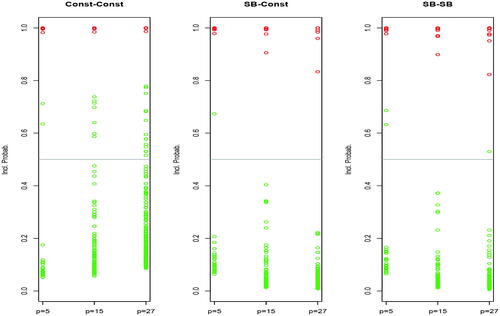
Experiment 1 shows that both possibilities for $f(\mathit{\gamma },\mathit{\delta })$ do a very good job at detecting active factors. However, the behavior with respect to spurious factors is quite different, and clearly confirms that the result encountered by Scott and Berger (2010) with numerical variables also extends to the scenario with factors: the constant prior (11) does not control for multiplicity and the number of signals corresponding to spurious factors clearly increases with p. The number of false signals is kept under control with (12), where there is only one of such cases, corresponding to the smallest value of p. As a conclusion, (12) is more suitable, particularly in a problem with moderate to large p, leaving us with two possible choices, SBC and SBSB, which we next discuss.

In Experiment 1, we also computed inclusion probabilities for SBSB, obtaining the plot on the right side of Figure 1. We observe that increasing the number of factors barely has any impact on the results. We would then expect to be able to differentiate among (14) and (15) relying on the notion of multiplicity but now over the number of levels of each of the factors. In summary, we were expecting that as ${\mathcal{l}}_j$ increases, the chance of wrongly declaring false positive would increase with (14) while remaining approximately constant with (15). But the following small experiment contradicted this conjecture.

Experiment 2. We performed a simulation from the model (1) with n = 300 observations and p = 4 factors all with the same number of levels ${\mathcal{l}}_j=\mathcal{l}$. The first factor is active with only its first level having a coefficient different from zero: ${\mathit{\beta }}_1^{\top }=({\beta }_{11}, {\mathit{0}}^{\top })$, and all the other vectors of regression coefficients are null. We are interested in the effect on the inclusion probabilities of factors of increasing $\mathcal{l}$. For that reason, we have performed the experiment for $\mathcal{l}\in \{5,15\}$. To have a similar content of information with these varying $\mathcal{l}$, the first 30 individuals are assigned to the first level of the factor and the rest, namely 270, are randomly assigned to the remaining levels. For the spurious factors, the assignment is random. The results for the inclusion probabilities of the factors for two values of β₁₁ are in Table 1. We clearly observe that both priors behave similarly when the number of levels is small. More difficult to understand is why the proposals react differently to an increase on $\mathcal{l}$: SBC becomes quite more conservative, and the opposite behavior in SBSB.

Table 1 Results for Experiment 2, rounded to two decimal places.

	${\beta }_{11}=1.0$				${\beta }_{11}=0.9$
	SBSB		SBC		SBSB		SBC
	$\mathcal{l}=5$	$\mathcal{l}=15$	$\mathcal{l}=5$	$\mathcal{l}=15$	$\mathcal{l}=5$	$\mathcal{l}=15$	$\mathcal{l}=5$	$\mathcal{l}=15$
$p({\tau }_1=1|\mathit{y})$	1.00	1.00	1.00	1.00	0.86	0.98	0.87	0.64
$p({\tau }_2=1|\mathit{y})$	0.04	0.15	0.03	0.00	0.05	0.17	0.03	0.00
$p({\tau }_3=1|\mathit{y})$	0.08	0.18	0.07	0.00	0.09	0.20	0.07	0.01
$p({\tau }_4=1|\mathit{y})$	0.04	0.13	0.02	0.00	0.04	0.15	0.02	0.00

NOTE: The effect on the posterior inclusion probabilities of increasing the number of levels within factors.

The results in Experiment 2 are not compatible with the idea of multiplicity control, since posterior probabilities of inclusion of factors (either active or spurious) are clearly sensitive to a change in the number of levels. To provide a correct interpretation of these results, and later to discriminate between SBSB and SBC, we need to further analyze how these two different possibilities summarize the evidence that is attributed to the factors.

It is straightforward to see that the posterior distribution of $(\mathit{\gamma },\mathit{\tau })$ (which variables and factors are included in the model) is$$f(\mathit{\gamma },\mathit{\tau }|\mathit{y})=\frac{{\mathcal{B}}_{(\gamma ,\tau )} f(\mathit{\gamma },\mathit{\tau })}{\sum _{(\gamma \prime ,\tau \prime )}{\mathcal{B}}_{(\gamma \prime ,\tau \prime )} f(\mathit{\gamma }\prime ,\mathit{\tau }\prime )},$$where ${\mathcal{B}}_{(\gamma ,\tau )}$ is the weighted mean of Bayes factors for models in the set $\mathcal{M}(\mathit{\gamma },\mathit{\tau })$:$${\mathcal{B}}_{(\gamma ,\tau )}=\sum _{(\gamma ,\delta )\in \mathcal{M}(\gamma ,\tau )} B_{(\gamma ,\delta )} f(\mathit{\delta }|\mathit{\gamma },\mathit{\tau }).$$

Now, notice that the priors (14) and (15) apportion probabilities of models in $\mathcal{M}(\mathit{\gamma },\mathit{\tau })$ in a way that only depends on the dimension $\kappa (\mathit{\gamma },\mathit{\tau })$, hence allowing us to alternatively to write:(16) $$\begin{array}{c}{\mathcal{B}}_{(\gamma ,\tau )}=\sum _{r\in R(\gamma ,\tau )} \overline{\underset{\kappa (\gamma ,\delta )=r}{B_{(\gamma ,\delta )\in \mathcal{M}(\gamma ,\tau )}}}\times p[\kappa (\mathit{\gamma },\mathit{\delta })\\ =r|(\mathit{\gamma },\mathit{\delta })\in \mathcal{M}(\mathit{\gamma },\mathit{\tau })].\end{array}$$(16)

The quantity with the large bar is the average of the Bayes factors for models in $\mathcal{M}(\mathit{\gamma },\mathit{\tau })$ with dimension r (that ranges in the interval $R(\mathit{\gamma },\mathit{\tau })]$—see Result S.2 of Section S.4 of the supplementary materials for an explicit formula for this range). The second factor in the sum in (16) is the (prior) probability mass function of the dimension of a model in $\mathcal{M}(\mathit{\gamma },\mathit{\tau })$, so a simple transformation of either (14) (in the case of Constant prior) or (15) (for the Scott and Berger). As in the standard variable selection problem, it is straightforward to see that the Constant prior transforms into a bell shaped probability distribution over the dimensions, while the Scott and Berger is uniform. Hence, ${\mathcal{B}}_{(\gamma ,\tau )}$ is a weighted mean of the means of Bayes factors of each dimension with either weights directly proportional to the number of models in each dimension (constant) or constant weights (Scott and Berger).

Intuitively, ${\mathcal{B}}_{\gamma ,\tau }^C$ (${\mathcal{B}}_{(\gamma ,\tau )}$ with the constant prior) summarizes the evidence in favor of $\mathcal{M}(\mathit{\gamma },\mathit{\tau })$ using models of average dimension, while ${\mathcal{B}}_{\gamma ,\tau }^{SB}$ summarizes that evidence equally collecting information from all dimensions. Unless the true model is of average size in $\mathcal{M}(\mathit{\gamma },\mathit{\tau })$ the evidence reported by ${\mathcal{B}}_{\gamma ,\tau }^C$ is expected to be quite conservative (if the true model is of small dimension, then ${\mathcal{B}}_{\gamma ,\tau }^C$ is small because complex models are used as representative of the set; if, on the contrary, the true model is of large dimension, then ${\mathcal{B}}_{\gamma ,\tau }^C$ is small because the models used as representative do not fit well enough). On the contrary, the case of ${\mathcal{B}}_{\gamma ,\tau }^{SB}$ is robust since it uses representatives of all possible dimensions so it does not matter which is the dimension of the true model. These differences are not important when the cardinality of $\kappa (\mathit{\gamma },\mathit{\tau })$ is small (e.g., when the number of levels is small) but could be quite pronounced as the number of levels increase.

In retrospect, the above reasoning provides a clear explanation to the results in Table 1 about Experiment 2 (recall that here only one level in the first factor was active so models of moderate to large number of active levels are expected to be barely endorsed by the data). In the case of SBC, the inclusion probabilities of factors (either true or spurious) decrease not because it does a better job at rejecting false signals but rather because models of average size are quite bad models (recall that only one level in the first factor is active). The explanation for the increase in probabilities in SBSB is not on the prior (because it remains constant on the dimension) but on the pronounced decrease in Bayes factors associated with models of moderate to large numbers of active levels.

In summary, both SBSB and SBC provide the right control for multiplicity over the number of numerical variables and factors. The difference between the two are not expected to be important when the number of levels in the factors is small (say no larger than 5 or 6). When the number of levels increases, SBSB is more robust and will summarize the evidence in favor of factors in a more sensible way assigning equal weight to the contribution of all possible number of levels. On the contrary, SBC summarizes that evidence through models with an average number of levels. By default, our recommended choice is SBSB: (12) + (15), and it is the one that we implement in the remainder of the article.

4 A Comparison With Alternative Methods

A common way of assessing the performance of statistical methodologies is through their frequentist behavior, that is, how they fare in many repetitions of an experiment where the truth is known.

In variable selection, the frequentist behavior is measured in terms of the proportion of times a method detects true explanatory variables (true positives or sensitivity) and the proportion of times it rejects true inert ones (true negatives or specificity). Regarding our methodology (the one constructed in Section 3), which is model-selection based, several criteria can be established to decide whether a variable or factor is relevant. The two most popular, and that we further consider, are:

• Highest posterior probability model: A factor is declared relevant if at least one of its levels is included in the model with the largest posterior probability. We denote this criterion as DHPM (using the robust prior). When using the approximation (10) with (8), we label the criterion as BICHPM; with (9), we use the label AICHPM.

• Posterior inclusion probabilities: A factor is declared relevant if its posterior inclusion probability (3) is larger than 1/2. We denote this criterion as DIP (using the robust prior). When using the approximation (10) with (8), we label the criterion as BICIP; with (9), we use the label AICIP.

We compare the two strategies described above with several others that have been proposed to handle variable selection with factors. We do not claim to be exhaustive in the list of competing methods; our goal is to investigate how our method fares against some of the existing alternatives. For this, we have included representatives of Bayesian “model selection” methods and frequentist “estimation” methods (see Section 2). In particular, we have considered: Bayesian sparse group selection (BSGS by Lee and Chen (2015) implemented with the R package BSGS); effect Fusion (eF by Pauger and Wagner (2019) and Pauger, Leitner, and Wagner (2019) and R package effectFusion) and the three different penalties in group Lasso: grLasso (L2 penalty by Yian and Lin (2006)); grMCP (minimax concave penalty by Breheny and Huang (2009)), and grSCAD (smoothly clipped absolute deviation penalty by Fan and Li (2001)) all implemented with the R package grpreg. We have also considered CASANOVA (Bondell and Reich 2009) that, later in Section 5, we use for its simultaneous ability to identify groups within factors.

We also implemented the standard application of AIC and BIC, two readily available model selection criteria. We label BIC the procedure that results from choosing the model that minimizes (8). The same procedure but using (9) as the criterion, is labeled as AIC. This was implemented using the R package leaps (Lumley 2020).

For the experiment described below, we have run the different Bayesian methods a number of iterations taking similar amount of time. For each simulated dataset, obtaining the selected model in DHPM (DIP, and implemented approximations) took approximately (in a computer with 2.6GHz i5 CPU) 2.6 min (total of 60,000 iterations); in BSGS, 2.2 min (96,000 iterations) and 2.5 min for eF (200,000 iterations). For reproducibility, we used a fixed initial random seed and the code used is provided as supplementary materials. As a final observation, we ran the algorithms following what seemed to be the default recommendations and it is possible that more careful tuning would produce better results. Recall that our methodology is fully automatic, no tuning is necessary.

We followed a simulation scheme similar to the one in Pauger and Wagner (2019). In particular, we generated 500 datasets from the model (1) with $n\in \{150,250,500\}$ observations and p = 4 factors, denoted Λ_j . The first two factors have eight levels and the rest have four levels. For the regression parameter for ${\Lambda }_1$ and ${\Lambda }_3$ we considered two different possibilities: ${\mathit{\beta }}_1^{\top }=(0,0,1,1,1,1,-2,-2),{\mathit{\beta }}_3^{\top }=(0,0,2,2)$ and ${\mathit{\beta }}_1^{\top }=(0,0,0,0,0,0,0,-2),{\mathit{\beta }}_3^{\top }=(0,0,0,2)$, while ${\mathit{\beta }}_2=\mathit{0}$ and ${\mathit{\beta }}_4=\mathit{0}$ (so ${\Lambda }_2$ and ${\Lambda }_4$ are spurious, and ${\Lambda }_1$ and ${\Lambda }_3$ are active factors). The intercept was fixed at ${\beta }_0=1$ and the standard deviation of errors was σ = 1.

With respect to how the sampling units are distributed in the categories we consider two possibilities: one with a balanced design (equally likely to be in each level) and an unbalanced design in which each unit was randomly assigned to one of the categories in ${\Lambda }_1,{\Lambda }_2$ with probabilities $(0.10,0.10,0.20,0.05,0.20,0.10,0.20,0.05)$ and to the categories in ${\Lambda }_3,{\Lambda }_4$ with probabilities $(0.10,0.40,0.20,0.30).$ For the methodology in eF (Pauger and Wagner 2019), and as in their example, the first two factors are treated as nominal while the last two as ordinal.

Results are displayed in Table 2 in the form of proportion of true positives (for ${\Lambda }_1$ and ${\Lambda }_3$) and true negatives (for ${\Lambda }_2$ and ${\Lambda }_4$). In general, all methods perform very well in the detection of true active factors. The only situation where we see significant differences is for ${\Lambda }_1$ (only one active level out of eight) and the case where the design is unbalanced and n = 150. Here, AIC, BIC, grLasso, CASANOVA, and AICIP, exhibit a better performance, closely followed by BSGS, grSCAD and DIP, DHPM, BICIP, and BICHPM. In this case, the sensitivity of eF is small (0.53). The differences in specificity (proportion of true inert factors correctly identified) are more pronounced: in general, eF, DIP, DHPM, BICIP, and BICHPM classify with high precision. The specificity of AICHPM, CASANOVA, and BIC is lower but still high although CASANOVA seems to suffer as n decreases. Next, we have grMCP and grSCAD (which still behave reasonably well) and then grLasso, AICIP, and AIC with quite poor behavior.

Table 2 Proportion of true positives (for ${\Lambda }_1$ and ${\Lambda }_3$) and true negatives (for ${\Lambda }_2$ and ${\Lambda }_4$) for methods compared.

	Unbalanced ${\mathit{\beta }}_2={\mathit{\beta }}_4=\mathit{0}$
	${\mathit{\beta }}_1^{\top }=(0,0,1,1,1,1,-2,-2),{\mathit{\beta }}_3^{\top }=(0,0,2,2)$													${\mathit{\beta }}_1^{\top }=(0,0,0,0,0,0,0,-2),{\mathit{\beta }}_3^{\top }=(0,0,0,2)$
	n = 500					n = 250				n = 150				n = 500				n = 250				n = 150
	${\Lambda }_1$	${\Lambda }_2$		${\Lambda }_3$	${\Lambda }_4$	${\Lambda }_1$	${\Lambda }_2$	${\Lambda }_3$	${\Lambda }_4$	${\Lambda }_1$	${\Lambda }_2$	${\Lambda }_3$	${\Lambda }_4$	${\Lambda }_1$	${\Lambda }_2$	${\Lambda }_3$	${\Lambda }_4$	${\Lambda }_1$	${\Lambda }_2$	${\Lambda }_3$	${\Lambda }_4$	${\Lambda }_1$	${\Lambda }_2$	${\Lambda }_3$	${\Lambda }_4$
DIP	1	1		1	0.99	1	1	1	0.96	1	0.99	1	0.94	1	0.99	1	0.96	0.99	0.96	1	0.94	0.90	0.94	1	0.92
DHPM	1	1		1	0.99	1	1	1	0.99	1	1	1	0.99	1	1	1	0.99	0.99	1	1	0.99	0.83	0.99	1	0.99
BICIP	1	1		1	0.99	1	1	1	0.98	1	0.99	1	0.98	1	1	1	0.98	0.99	0.98	1	0.96	0.89	0.96	1	0.96
BICHPM	1	1		1	1	1	1	1	0.99	1	0.99	1	0.99	1	1	1	0.99	0.99	1	1	0.99	0.83	1	1	0.99
AICIP	1	0.69		1	0.40	1	0.65	1	0.36	1	0.60	1	0.30	1	0.68	1	0.41	1	0.67	1	0.41	0.98	0.63	1	0.42
AICHPM	1	0.98		1	0.94	1	0.96	1	0.91	1	0.94	1	0.91	1	0.98	1	0.94	0.99	0.96	1	0.94	0.92	0.95	1	0.94
BSGS	1	0.97		1	0.78	1	0.96	1	0.86	1	0.93	1	0.89	1	0.97	1	0.79	1	0.95	1	0.81	0.95	0.91	1	0.86
grLasso	1	0.18		1	0.28	1	0.21	1	0.25	1	0.24	1	0.28	1	0.21	1	0.32	1	0.29	1	0.39	0.99	0.34	1	0.44
eF	1	1		1	0.96	1	1	1	0.93	1	1	1	0.93	1	1	1	0.97	0.89	1	1	0.94	0.56	1	1	0.94
grMCP	1	0.91		1	0.91	1	0.88	1	0.88	1	0.89	1	0.89	1	0.85	1	0.82	0.99	0.83	1	0.78	0.91	0.79	1	0.78
grSCAD	1	0.87		1	0.86	1	0.83	1	0.83	1	0.81	1	0.79	1	0.63	1	0.62	1	0.56	1	0.57	0.94	0.56	1	0.60
CASANOVA	1	0.75		1	0.94	1	0.50	1	0.80	1	0.34	1	0.71	1	0.95	1	0.99	1	0.78	1	0.93	0.98	0.59	1	0.84
BIC	1	0.92		1	0.95	1	0.91	1	0.97	1	0.92	1	0.97	1	0.9	1	0.97	1	0.87	1	0.96	1	0.88	1	0.96
AIC	1	0.34		1	0.60	1	0.28	1	0.62	1	0.29	1	0.58	1	0.28	1	0.58	1	0.30	1	0.59	1	0.27	1	0.61
	Balanced ${\mathit{\beta }}_2={\mathit{\beta }}_4=\mathit{0}$
	${\mathit{\beta }}_1^{\top }=(0,0,1,1,1,1,-2,-2),{\mathit{\beta }}_3^{\top }=(0,0,2,2)$													${\mathit{\beta }}_1^{\top }=(0,0,0,0,0,0,0,-2),{\mathit{\beta }}_3^{\top }=(0,0,0,2)$
	n = 500					n = 250				n = 150				n = 500				n = 250				n = 150
	${\Lambda }_1$		${\Lambda }_2$	${\Lambda }_3$	${\Lambda }_4$	${\Lambda }_1$	${\Lambda }_2$	${\Lambda }_3$	${\Lambda }_4$	${\Lambda }_1$	${\Lambda }_2$	${\Lambda }_3$	${\Lambda }_4$	${\Lambda }_1$	${\Lambda }_2$	${\Lambda }_3$	${\Lambda }_4$	${\Lambda }_1$	${\Lambda }_2$	${\Lambda }_3$	${\Lambda }_4$	${\Lambda }_1$	${\Lambda }_2$	${\Lambda }_3$	${\Lambda }_4$
DIP	1		1	1	1	1	0.99	1	0.97	1	0.99	1	0.92	1	0.99	1	0.98	1	0.96	1	0.94	1	0.93	1	0.92
DHPM	1		1	1	1	1	0.99	1	1	1	0.99	1	0.98	1	1	1	1	1	0.99	1	0.99	1	0.99	1	1
BICIP	1		1	1	1	1	0.99	1	0.99	1	0.99	1	0.97	1	1	1	0.98	1	0.97	1	0.96	1	0.96	1	0.93
BICHPM	1		1	1	1	1	0.99	1	1	1	0.99	1	0.98	1	1	1	1	1	0.99	1	0.99	1	0.99	1	1
AICIP	1		0.68	1	0.41	1	0.67	1	0.40	1	0.59	1	0.36	1	0.64	1	0.42	1	0.61	1	0.39	1	0.60	1	0.34
AICHPM	1		0.96	1	0.94	1	0.97	1	0.93	1	0.94	1	0.90	1	0.98	1	0.95	1	0.96	1	0.92	1	0.95	1	0.92
BSGS	1		0.92	1	0.79	1	0.95	1	0.87	1	0.91	1	0.87	1	0.95	1	0.89	1	0.94	1	0.91	1	0.94	1	0.91
grLasso	1		0.20	1	0.26	1	0.19	1	0.31	1	0.24	1	0.33	1	0.19	1	0.31	1	0.21	1	0.29	1	0.25	1	0.34
eF	1		1	1	0.98	1	1	1	0.94	1	1	1	0.93	1	1	1	0.98	1	1	1	0.96	0.99	1	1	0.94
grMCP	1		0.89	1	0.90	1	0.91	1	0.91	1	0.88	1	0.89	1	0.91	1	0.91	1	0.85	1	0.85	1	0.84	1	0.83
grSCAD	1		0.85	1	0.86	1	0.85	1	0.84	1	0.82	1	0.79	1	0.81	1	0.81	1	0.70	1	0.67	1	0.57	1	0.59
CASANOVA	1		0.78	1	0.93	1	0.53	1	0.81	1	0.36	1	0.69	1	0.98	1	0.99	1	0.88	1	0.96	1	0.67	1	0.87
BIC	1		0.86	1	0.92	1	0.84	1	0.94	1	0.80	1	0.91	0.99	0.79	1	0.94	1	0.79	1	0.93	1	0.84	1	0.94
AIC	1		0.28	1	0.55	1	0.29	1	0.59	1	0.29	1	0.61	1	0.26	1	0.63	1	0.26	1	0.58	1	0.26	1	0.58

NOTE: The dashed line separates methods based on our considerations (definition of $\mathcal{M}$ and SBSB prior over the model space) and existing methods.

The take-home message from this experiment is that, as expected, no method is superior to all the others. However, the methods we ultimately recommend, namely DIP and DHPM, perform uniformly (in all scenarios) quite satisfactorily. Unsurprisingly, their natural approximations, BICIP and BICHPM, perform also quite well. Notice that we are only measuring the frequentist performance of these methods. From a theoretical perspective, the robust prior used in DIP and DHPM present a number of very attractive properties in the context of variable selection which are not possible to assess in a frequentist simulation study—see Bayarri et al. (2012).

5 Merging Levels

When, in a given model $(\mathit{\gamma },\mathit{\delta })$, the effects of certain levels within a factor are exactly equal (and different from zero), these levels can be merged and that model can be reparameterized using a smaller number of parameters, hence providing the same fit at a lower cost. Our methodology cannot accommodate this situation because the reduced model is not in $\mathcal{M}$; the evidence in favor of the factor that we compute is the one given by the more complex model $(\mathit{\gamma },\mathit{\delta })$. This implies, in principle, a loss of power in our methodology compared to a hypothetical one in which the model space contains all possible combinations of coincident levels. Such loss of power would come from the extra dimensionality our method would need in this situation. To get an idea of this potential loss, we performed a simulation where our proposal is compared with an oracle-informed methodology that knows how the different levels are grouped in the data. The results are very satisfactory even with a large level of aggregation; we relegate the details to the supplementary materials, Section S.6. For methods specifically conceived to detect levels with a common effect—usually called “subgroup identification”—the reader is referred to Berger, Wang, and Shen (2014) and Pauger and Wagner (2019).

Nevertheless, we propose a grouping strategy that is applicable after computing the posterior distribution on $\mathcal{M}$. First, obtain the highest posterior model; it is under this model that we will produce a grouping of the levels. Of course, the levels of the factors Λ_j such ${\tau }_j=0$ are all in a single group. For factors Λ_j such that ${\tau }_j=1$, the levels that are not included in this model, that is, the ones that correspond to the components of ${\mathit{\delta }}_j$ that are zero, are all in a single group. For the remainder, compute credible intervals at a specified level for the effects ${\beta }_{jr}-{\beta }_0$; two levels of factor Λ_j are in the same group if their corresponding intervals overlap.

To assess the performance of this strategy, we have implemented it in the context of the simulations of Section 4 and compared the results with those obtained using eF (effect Fusion) and CASANOVA (both methods conceived for grouping). Recall that, in this simulation, two of the factors are inactive (${\Lambda }_2$ and ${\Lambda }_4$) so the ability to detect that these levels conform a single group is implicitly contained in Table 2 while for the active factors ${\Lambda }_1$ and ${\Lambda }_3$ we have considered two possibilities due to the definitions of ${\mathit{\beta }}_1$ and ${\mathit{\beta }}_3$. In the first scenario ${\Lambda }_1$ has three groups $\left\{\right\{1,2\},\{3,4,5,6\},\{7,8\left\}\right\}$ while ${\Lambda }_3$ has two: $\left\{\right\{1,2\},\{3,4\left\}\right\}$. In the second scenario both have two groups: for ${\Lambda }_1$ we have $\left\{\right\{1,2,3,4,5,6,7\},\{8\left\}\right\}$ and for ${\Lambda }_3$ $\left\{\right\{1,2,3\},\{4\left\}\right\}$. For the 500 datasets simulated in each configuration, we retain the frequency of times each method detects the true grouping.

The results we obtained are collected in Table 3, where we have used the same labeling as in the experiment in the previous section. The method that we recommend, DHPM, and its approximation, BICHPM, with 95% credible intervals, behave quite similarly and show a very satisfactory performance. In general, these outperform CASANOVA. Our methods and eF, which is designed specifically to merge levels of factors, exhibit a very similar performance. As expected, all methods diminish their classification power as the sample size decreases, the number of groups in a factor increases and when the design is unbalanced. Also, AICHPM is not competitive, as the results obtained are clearly worse than the others.

Table 3 Proportion of groups truly detected based on HPM and overlapping of 95% credible intervals.

	Unbalanced ${\mathit{\beta }}_2={\mathit{\beta }}_4=\mathit{0}$
	${\mathit{\beta }}_1^{\top }=(0,0,1,1,1,1,-2,-2)$						${\mathit{\beta }}_1^{\top }=(0,0,0,0,0,0,0,-2)$
	${\mathit{\beta }}_3^{\top }=(0,0,2,2)$						${\mathit{\beta }}_3^{\top }=(0,0,0,2)$
	n = 500		n = 250		n = 150		n = 500		n = 250		n = 150
	${\Lambda }_1$	${\Lambda }_3$	${\Lambda }_1$	${\Lambda }_3$	${\Lambda }_1$	${\Lambda }_3$	${\Lambda }_1$	${\Lambda }_3$	${\Lambda }_1$	${\Lambda }_3$	${\Lambda }_1$	${\Lambda }_3$
DHPM	0.89	0.96	0.37	0.94	0.08	0.93	0.98	0.95	0.95	0.97	0.79	0.94
BICHPM	0.91	0.96	0.41	0.94	0.09	0.93	0.98	0.96	0.95	0.97	0.80	0.95
AICHPM	0.55	0.96	0.09	0.95	0.00	0.93	0.80	0.90	0.79	0.92	0.66	0.89
eF	0.88	0.98	0.30	0.95	0.05	0.92	1.00	0.96	0.89	0.92	0.56	0.92
CASANOVA	0.24	0.77	0.09	0.60	0.08	0.50	0.93	0.96	0.74	0.90	0.54	0.79
	Balanced ${\mathit{\beta }}_2={\mathit{\beta }}_4=\mathit{0}$
	${\mathit{\beta }}_1^{\top }=(0,0,1,1,1,1,-2,-2)$						${\mathit{\beta }}_1^{\top }=(0,0,0,0,0,0,0,-2)$
	${\mathit{\beta }}_3^{\top }=(0,0,2,2)$						${\mathit{\beta }}_3^{\top }=(0,0,0,2)$
	n = 500		n = 250		n = 150		n = 500		n = 250		n = 150
	${\Lambda }_1$	${\Lambda }_3$	${\Lambda }_1$	${\Lambda }_3$	${\Lambda }_1$	${\Lambda }_3$	${\Lambda }_1$	${\Lambda }_3$	${\Lambda }_1$	${\Lambda }_3$	${\Lambda }_1$	${\Lambda }_3$
DHPM	0.92	0.93	0.53	0.95	0.17	0.94	0.98	0.97	0.97	0.96	0.91	0.93
BICHPM	0.92	0.94	0.58	0.95	0.20	0.94	0.98	0.97	0.97	0.97	0.92	0.94
AICHPM	0.81	0.94	0.14	0.96	0.03	0.93	0.82	0.89	0.79	0.91	0.72	0.88
eF	0.94	0.96	0.54	0.95	0.13	0.92	1.00	0.98	1.00	0.96	0.99	0.96
CASANOVA	0.26	0.73	0.14	0.62	0.07	0.50	0.97	0.99	0.84	0.93	0.64	0.84

NOTE: The dashed line separates methods based on our considerations (definition of $\mathcal{M}$ and SBSB prior over the model space) and existing methods.

Supplementary Materials

Supplement Contains material that is not essential to the understanding of the methodology but adds insight, including a real application. It also includes proofs and the statement of technical results, as referenced in the article.

R-code In the interest of reproducibility, we include the R code necessary to obtain all the results and simulations provided in the article.

Additional information

Funding

This work was partially developed while both authors were visiting the Statistical and Applied Mathematical Sciences Institute, and hence it is partially supported by the National Science Foundation under Grant DMS-1638521. Gonzalo García-Donato has been partially supported by the project PID2019-104790GB-I00 from the Ministerio de Ciencia e Innovación (Spain) and by the project SBPLY/17/180501/000491 from the Consejeria de Educacion, Cultura y Deportes de la Junta de Comunidades de Castilla-La Mancha (Spain). Rui Paulo was partially supported by the Project CEMAPRE/REM—UIDB/05069/2020—financed by FCT/MCTES through national funds, and by the sabbatical fellowship SFRH/BSAB/142992/2018 attributed by FCT.

References

- Akaike, H. (1974), “A New Look at the Statistical Model Identification,” IEEE Transactions on Automatic Control, 19, 716–723. DOI: 10.1109/TAC.1974.1100705.
- Bayarri, M. J., Berger, J. O., Forte, A., and García-Donato, G. (2012), “Criteria for Bayesian Model Choice With Application to Variable Selection,” The Annals of Statistics, 40, 1550–1577. DOI: 10.1214/12-AOS1013.
- Bayarri, M. J., and García-Donato, G. (2007), “Extending Conventional Priors for Testing General Hypotheses in Linear Models,” Biometrika, 94, 135–152. DOI: 10.1093/biomet/asm014.
- Berger, J. O., and Pericchi, L. R. (2001), Objective Bayesian Methods for Model Selection: Introduction and Comparison, Lecture Notes–Monograph Series (Vol. 38), Beachwood, OH: Institute of Mathematical Statistics, pp. 135–207.
- Berger, J. O., Wang, X., and Shen, L. (2014), “A Bayesian Approach to Subgroup Identification,” Journal of Biopharmaceutical Statistics, 24, 110–129. DOI: 10.1080/10543406.2013.856026.
- Bondell, H., and Reich, B. (2009), “Simultaneous Factor Selection and Collapsing Levels in ANOVA,” Biometrics, 65, 169–177. DOI: 10.1111/j.1541-0420.2008.01061.x.
- Breheny, P., and Huang, J. (2009), “Penalized Methods for Bi-Level Variable Selection,” Statistics and Its Interface, 2, 369–380. DOI: 10.4310/sii.2009.v2.n3.a10.
- Castillo, I., Schmidt-Hieber, J., and Van Der Vaart, A. (2015), “Bayesian Linear Regression With Sparse Priors,” The Annals of Statistics, 43, 1986–2018. DOI: 10.1214/15-AOS1334.
- Chen, J., and Chen, Z. (2008), “Extended Bayesian Information Criteria for Model Selection With Large Model Spaces,” Biometrika, 95, 759– 771. DOI: 10.1093/biomet/asn034.
- Chen, R.-B., Chi-Hsiang, C., Yuan, S., and Wu, Y. (2016), “Bayesian Sparse Group Selection,” Journal of Computational and Graphical Statistics, 25, 665–683. DOI: 10.1080/10618600.2015.1041636.
- Chipman, H. (1996), “Bayesian Variable Selection With Related Predictors,” The Canadian Journal of Statistics/La Revue Canadienne de Statistique, 24, 17–36. DOI: 10.2307/3315687.
- Clyde, M., and Parmigiani, G. (1998), “Protein Construct Storage: Bayesian Variable Selection and Prediction With Mixtures,” Journal of Biopharmaceutical Statistics, 8, 431–443. DOI: 10.1080/10543409808835251.
- Desboulets, L. D. (2018), “A Review on Variable Selection in Regression Analysis,” Econometrics, 6, 1–27. DOI: 10.3390/econometrics6040045.
- Fan, J., and Li, R. (2001), “Variable Selection via Nonconcave Penalized Likelihood and Its Oracle Properties,” Journal of American Statistical Association, 96, 1348–1360. DOI: 10.1198/016214501753382273.
- Farcomeni, A. (2010), “Bayesian Constrained Variable Selection,” Statistica Sinica, 20, 1043–1062.
- Fernández, C., Ley, E., and Steel, M. F. (2001), “Benchmark Priors for Bayesian Model Averaging,” Journal of Political Economics, 100, 381–427. DOI: 10.1016/S0304-4076(00)00076-2.
- Fernández, C., Ley, E., and Steel, M. F. (2002), “Bayesian Modeling of Catch in a North-West Atlantic Fishery,” Applied Statistics, 51, 257–280.
- Friedman, J. H., Hastie, T., and Tibshirani, R. (2010), “Regularization Paths for Generalized Linear Models via Coordinate Descent,” Journal of Statistical Software, 33, 1–22. DOI: 10.18637/jss.v033.i01.
- George, E. I., and McCulloch, R. E. (1993), “Variable Selection via Gibbs Sampling,” Journal of the American Statistical Association, 88, 881–889. DOI: 10.1080/01621459.1993.10476353.
- Lee, K.-J., and Chen, R.-B. (2015), “BSGS: Bayesian Sparse Group Selection,” The R Journal, 7, 122–133. DOI: 10.32614/RJ-2015-025.
- Liang, F., Paulo, R., Molina, G., Clyde, M. A., and Berger, J. O. (2008), “Mixtures of g-Priors for Bayesian Variable Selection,” Journal of the American Statistical Association, 103, 410–423. DOI: 10.1198/016214507000001337.
- Lumley, T. (2020), “leaps: Regression Subset Selection,” R Package Version 3.1.
- Pauger, D., Leitner, M., and Wagner, H. (2019), “effectFusion: Bayesian Effect Fusion for Categorical Predictors.”
- Pauger, D., and Wagner, H. (2019), “Bayesian Effect Fusion for Categorical Predictors,” Bayesian Analysis, 14, 341–369. DOI: 10.1214/18-BA1096.
- Raman, S., Fuchs, T. J., Wild, P. J., Dahs, E., and Roth, V. (2009), “The Bayesian Group-Lasso for Analyzing Contingency Tables,” in Proceedings of the 26th International Conference on Machine Learning. DOI: 10.1145/1553374.1553487.
- Schwarz, G. (1978), “Estimating the Dimension of a Model,” The Annals of Statistics, 6, 461–464. DOI: 10.1214/aos/1176344136.
- Scott, J. G., and Berger, J. O. (2010), “Bayes and Empirical-Bayes Multiplicity Adjustment in the Variable-Selection Problem,” The Annals of Statistics, 38, 2587–2619. DOI: 10.1214/10-AOS792.
- Steel, M. F. (2020), “Model Averaging and Its Use in Economics,” Journal of Economic Literature, 58, 644–719. DOI: 10.1257/jel.20191385.
- Yian, M., and Lin, Y. (2006), “Model Selection and Estimation in Regression With Grouped Variables,” Journal of the Royal Statistical Society, Series B, 68, 49–67. DOI: 10.1111/j.1467-9868.2005.00532.x.
- Zellner, A., and Siow, A. (1980), “Posterior Odds Ratio for Selected Regression Hypotheses,” in Bayesian Statistics 1, eds. J. M. Bernardo, M. DeGroot, D. Lindley, and A. F. M. Smith, Valencia: University Press, pp. 585–603.