Capture-Recapture Models with Heterogeneous Temporary Emigration

ABSTRACT

We propose a novel approach for modeling capture-recapture (CR) data on open populations that exhibit temporary emigration, while also accounting for individual heterogeneity to allow for differences in visit patterns and capture probabilities between individuals. Our modeling approach combines changepoint processes—fitted using an adaptive approach—for inferring individual visits, with Bayesian mixture modeling—fitted using a nonparametric approach—for identifying clusters of individuals with similar visit patterns or capture probabilities. The proposed method is extremely flexible as it can be applied to any CR dataset and is not reliant upon specialized sampling schemes, such as Pollock’s robust design. We fit the new model to motivating data on salmon anglers collected annually at the Gaula river in Norway. Our results when analyzing data from the 2017, 2018, and 2019 seasons reveal two clusters of anglers—consistent across years—with substantially different visit patterns. Most anglers are allocated to the “occasional visitors” cluster, making infrequent and shorter visits with mean total length of stay at the river of around seven days, whereas there also exists a small cluster of “super visitors,” with regular and longer visits, with mean total length of stay of around 30 days in a season. Our estimate of the probability of catching salmon whilst at the river is more than three times higher than that obtained when using a model that does not account for temporary emigration, giving us a better understanding of the impact of fishing at the river. Finally, we discuss the effect of the COVID-19 pandemic on the angling population by modeling data from the 2020 season. Supplementary materials for this article are available online.

KEYWORDS:

• Angling
• Chinese restaurant process
• Clustering
• Population size
• Stopover model

1 Introduction

Capture-recapture (CR) data provide a method for monitoring wildlife populations, or more generally populations for which a census is infeasible because the probability of detecting individuals is lower than one. Appropriate means for capturing individuals are employed in a series of capture occasions. During these capture occasions, newly caught individuals are uniquely marked and all caught individuals are released back into the population. Repeating the process T times gives rise to a capture history, of length T, for each caught individual with entries equal to one (zero) indicating the capture occasions at which the particular individual was caught (not caught). At the end of the study, there remains an unknown number of individuals that were never caught and hence have capture histories with all entries equal to zero.

There exists a rich literature dealing with models for CR data. This covers closed-population models, which assume that the same individuals are present and available for capture at all T occasions (Darroch 1958; Otis et al. 1978; Pledger 2000), open-population models that allow for arrivals and departures during the study (Jolly 1965; Seber 1965; Schwarz and Arnason 1996; Pledger et al. 2009; Lyons et al. 2016) and a recent body of work exploring Bayesian nonparametric methods for CR data (Manrique-Vallier 2016; Matechou and Caron 2017, closed and open populations, respectively).

Typically, one of the assumptions of open-population CR models is that emigration is permanent; once individuals depart they are assumed to never arrive again. However, the assumption of permanent emigration is not always satisfied. Existing approaches for modeling temporary emigration in population ecology (see e.g., Zhou et al. 2019) so far mostly use Pollock’s robust design (Pollock 1982), which assumes that there are two types of sampling periods: primary periods, for example seasons, between which the population is open, and secondary periods, for example sampling days within a season, between which the population is closed. Clearly, there exist cases where methods relying on Pollock’s robust design cannot be employed.

In this article we propose a novel solution for modeling temporary emigration for CR data by developing a flexible, general and mathematically tractable Bayesian mixture model that also accounts for individual heterogeneity in the visit pattern and capture probability. We treat the visit history of each individual as a changepoint process with visits, when an individual transitions from nonpresent to present, signifying a changepoint. We model the corresponding departure times as dependent on these changepoints and we extend recently developed adaptive MCMC methods (Benson and Friel 2018) for updating the number and position of changepoints of each individual. These adaptive methods provide us with an elegant and computationally efficient way to infer individual visit histories, without requiring any tuning or complicated proposal distributions.

Additionally, we model individual heterogeneity using a random finite measure as the intensity of a Poisson process that jointly models the number of individuals and their visit histories. Conditionally on the number of individuals, the visit histories are shown to be a sample from a mixture model, which, although technically is finite dimensional, we fit using Bayesian nonparametric techniques. Our approach builds upon recent work by Argiento and De Iorio (2022) that exploits the relationship between finite and infinite mixtures in a Bayesian framework. Argiento and De Iorio (2022) show that a mixture model with a random number of components is indeed a nonparametric model since its complexity is a-priori unbounded and inferred by the data. Moreover, while an infinite mixture model can lead to an a posteriori inconsistency on the estimation of the number of clusters (Miller and Harrison 2018), this is not the case for finite mixture models with a random number of components. The use of a finite mixture model allows us to devise a blocked conditional Gibbs sampler, which is faster than the marginal algorithms that are usually adopted, as in Matechou and Caron (2017). Finally, we show that when the number of elements being clustered is itself random, the clustering can be expressed via a function, which we call N-exchangeable random probability function, that can be used to derive the marginal distribution of N, and gives rise to an interpretation of the clustering in terms of the Chinese restaurant process.

Our proposed modeling approach has several distinctive advantages. In contrast to methods relying on Pollock’s robust design, we do not need to assume population closure. From a computational point of view, we design an adaptive scheme for the changepoint process part of the model that is free from complicated tuning strategies and we tackle the mixture model from a Bayesian point of view via a conditional algorithm that is computationally efficient and allows for full Bayesian inference.

We fit our model to CR data on salmon anglers in Norway. The anglers only report a visit to the river on a particular day if they catch at least one salmon. This gives rise to a standard CR dataset indicating the days when each angler reported a catch. However, the number of anglers who visited the river, the number of days on which they were present each season and their probability of catching salmon whilst at the river are unknown. Our results in terms of types of visit patterns and fishing abilities are consistent across the 2017, 2018, and 2019 seasons. Specifically, we identify two clusters, with the largest cluster, consisting of around 95% of the angler population, making two to three visits on average each year, which last for around two days on average. The second cluster of anglers make around eight visits each year, each lasting on average two to three days. This leads to substantial differences in the total number of days spent at the river on average between the two clusters. Additionally, we estimate that the total number of anglers who visited the river each year is considerably higher than the number of anglers who caught at least one salmon, and, for the first time in the Gaula river, we estimate the total number of anglers who are present at the river on each day of the season. Finally, we quantify the effect of the COVID-19 pandemic on the angling population by analyzing the 2020 season data. Our findings suggest that there was a considerable increase in the number of anglers who visited that year, with anglers spending longer on average per visit compared to previous seasons but having an overall lower ability to catch fish. Such information is invaluable for managing the river, and correctly and precisely setting fishing quotas and introducing further regulations, as required.

We present the model in Section 3 and discuss its clustering behavior in Section 4. Our algorithm used for inference, including the adaptive MCMC changepoint sampler and the Bayesian nonparametric algorithm used for clustering, is presented in Section 5. The results from fitting the model to simulated data and to the angler data are presented in Section 6 while the article concludes in Section 7. Additional technical details about our model and algorithm, as well as results of an extensive simulation study, are provided in the supplementary materials.

2 Salmon Angler Data

The Gaula is an unregulated river in Norway that is a very popular destination for salmon anglers. Any catches of salmon have to be reported by the anglers to the river management board. However, individual anglers only report that they were fishing on a particular day of the season, which lasts for T = 92 (1st of June to 31st of August) days, if they catch at least one salmon that day. This creates a capture history, which is a vector of length T, for each angler, with entry t equal to one if the angler caught salmon on day t, and zero otherwise, with $t=1,\dots ,T$. There also exists an unknown number of anglers who visited the river but did not catch salmon, and hence share the capture history with all T entries equal to 0. The population is open, with anglers entering and exiting the river throughout the season. Anglers need to purchase fishing licenses from land owners along the river in advance, but the information on the number of licenses that have been sold each year is considered sensitive and not shared. Licenses are often sold-out months in advance, and the only restriction placed on anglers is that they can only remove a maximum of four salmon a year for the period we are considering in this article. However, they can catch as many salmon as they want and release them back in the river.

Individual anglers can return to the river to fish an arbitrary number of times in the season, meaning that their emigration from the site needs to be treated as temporary. Clearly, we cannot employ methods relying on Pollock’s robust design in this case as the population cannot be assumed closed for any period in the season. Additionally, our inference needs to account for individual heterogeneity in the visit behavior and fishing ability, the latter expressed through the probability of an angler catching salmon whilst at the river, and hence being themselves “caught,” henceforth referred to as observed, while present at the river. For example, some anglers may visit often for shorter periods of time while others may visit less regularly for longer periods of time, with capture probability also linked to the visit behavior, with, for example, frequent visitors being more skilled in fishing and vice versa.

We are interested in inferring the size of the population of anglers, N, and the visit history of each angler, which consists of the number, timing and duration of their visits, as well as the probability of an angler catching salmon on any given day. We note here that if an open population model that does not allow for temporary emigration is fitted to the data, such as the “POPAN” model in the R package RMark (Laake 2013), then the resulting estimates of capture probability, which are between 0.06 and 0.07 for all years, are certainly under-estimates; since the model assumes that individuals are present between their first and last observation, it inevitably underestimates the probability of capture.

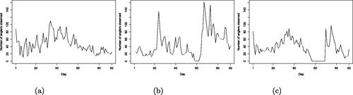
The total number of anglers observed in the 2017, 2018, and 2019 seasons is equal to 2057, 1901, and 1687, respectively, but we cannot infer the total number of visitors to the river each season using the raw data alone. The median number of times that each angler has been observed is equal to one in 2017 and 2019 and to two in 2018 but it is not possible to decipher from the data alone the total number of days each angler has spent at the river. Similarly, the number of visits made by individual anglers each year is unknown. Clearly, we can safely assume that consecutive days on which an individual angler was observed belong to a single visit. However, observations of individual anglers are also separated by days on which the particular angler was not observed. If we assume that visits are separated by at least one day of non-observation, then we find that the proportion of anglers making a single visit would be set to around 60% with an average visit length of around 1.2 days for all seasons, while if we assume that visits are separated by at least two days of non-observation, then these figures change to around 70% and 1.4–1.5 days on average. Finally, Figure 1 shows that the pattern in the number of anglers observed each day of the season varies greatly between years, but it is of interest to compare the arrival and departure patterns between years, which cannot be achieved using the raw capture histories. These questions motivate the development of the model presented in Section 3.

Fig. 1 Number of anglers observed each day of the season in 2017, (a), 2018, (b), and 2019, (c). The river may be closed occasionally for fishing, which results in days when no fish are caught, such as the days around day 60 in 2018 and in 2019.

Inferring the number of anglers present at any one time within the season enables the river management to assess the fishing pressure and consequently decide on fishing quotas or additional regulations. Information on the probability of catching salmon is valuable to the river management board for the purposes of fisheries management, for ensuring the conservation of salmon in the river and the availability of resources, such as accommodation and food, for anglers. Knowledge about the number of anglers who visit the river each season and the number of visits they each make can help demonstrate to local politicians and stakeholders the importance and attractiveness of the river Gaula as a tourist destination and increase the appreciation of the value of salmon fishing to the local community, resulting in policies that ensure protection and conservation of the river and the salmon stock. Finally, by modeling the 2020 season and quantifying the differences compared to previous seasons in terms of numbers of visitors, visit patterns and capture probabilities can shed light on the effect of the COVID-19 pandemic and the corresponding global travel restrictions on the angling and hence salmon population at the Gaula river.

3 Model

We denote the number of individuals caught at least once by n and the number of sampling occasions by T. The population size is denoted by N. Let $i=1,\dots ,N$ index individuals and $t=1,\dots ,T$, which we refer to as time, index equally spaced sampling occasions.

The data consist of n capture histories, each of length T. We denote the capture history of individual i by $\mathbf{C}{\mathbf{H}}_i$ with entry ${\text{CH}}_{it}=1$ if individual i was caught at time t and 0 otherwise. Individuals with index $n+1,\dots ,N$ have capture histories with all entries equal to 0.

Individual i, $i=1,\dots ,N$, makes an unknown number of visits, k_i, and has an unknown visit history summarized by the arrival times ${\mathit{a}}_i=(a_{i1},a_{i2},\dots ,a_{i{k}_i})$ and the corresponding departure times ${\mathit{d}}_i=(d_{i1},d_{i2},\dots ,d_{i{k}_i})$. The arrival times are an increasing sequence of length k_i with $k_i>0\forall i$, in $\{1,\dots ,T\}$ and the corresponding departure times are an increasing sequence in $\{1,\dots ,T\}$, such that $a_{iv}\le d_{iv}<a_{iv+1}$ for each $v=1,\dots ,k_i$, with $a_{k_i+1}=T+1$ by definition. The visit history uniquely defines a corresponding presence history, with the presence history of individual i denoted by $\mathbf{P}{\mathbf{H}}_i$ and ${\text{PH}}_{it}=1$ if individual i was present at time t and 0 otherwise. For example in Figure 2, the presence history $\mathbf{P}{\mathbf{H}}_i$ is coded as a sequence of 0s (absent) and 1s (present) and represented by a piecewise constant function. In this case we have k_i = 2 visits, $a_{i1}=27$ and $a_{i2}=57$, corresponding to the points where the piecewise constant function jumps from 0 to 1, represented by the two filled circles on the x-axis, and k_i = 2 departure times, $d_{i1}=56$ and $d_{i2}=86$, corresponding to the points where the function jumps from 1 to 0, represented by the two filled triangles on the x-axis. We observe that, as mentioned above, ${\mathit{a}}_i$ and ${\mathit{d}}_i$ uniquely define $\mathbf{P}{\mathbf{H}}_i$, but not vice versa. Nevertheless, to simplify notation, in the following we use $\mathbf{P}{\mathbf{H}}_i\equiv ({\mathit{a}}_i,{\mathit{d}}_i)$, since it is the latter that we infer.

Fig. 2 Example presence history for individual i. Gray ticks indicate external points, ${\mathcal{E}}_i$, black ticks indicate internal points, ${\mathcal{I}}_i$, solid circles indicate changepoints, that is, arrivals times, ${\mathcal{A}}_i$, and solid triangles indicate their corresponding departure times, ${\mathcal{D}}_i$. The arrival and departure times are indicated on the x-axis.

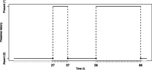
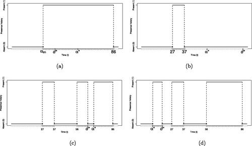
Fig. 3 Four examples of presence histories that can lead to the presence history shown in Figure 2: (a) Split move; we propose an internal point as a new changepoint ( $a^{\star }=56$), which forms a visit with the next available departure point (d_im = 86), while the existing previous arrival time a_im = 27 forms a visit with the newly proposed departure time ( $d^{\star }=37$), (b) Add move; we propose an external point as a new changepoint ( $a^{\star }=56$), which forms a visit with the newly proposed departure time ( $d^{\star }=86$), (c) Merge move; we propose to delete an existing changepoint ( $a^{\star }=70$) and the departure time of the previous visit ( $d^{\star }=56$), so the two visits are merged, and (d): Delete move: we propose to delete an existing changepoint ( $a^{\star }=11$) and its corresponding departure time ( $d^{\star }=19$).

We refer to the set $\left\{(\mathbf{PH},\mathbf{CH})\right\}:=\{(\mathbf{P}{\mathbf{H}}_i,\mathbf{C}{\mathbf{H}}_i),i=1,\dots ,N\}$ as the augmented data because it includes both the $1,\dots ,n$ caught individuals and the $n+1,\dots ,N$ uncaught individuals. We note that each observation $(\mathbf{P}{\mathbf{H}}_i,\mathbf{C}{\mathbf{H}}_i)$ is a pair of sequences such that its tth entry is (CH_it,PH ${}_{it})\in \{0,1\}\times \{0,1\}$. We denote by $(\mathcal{P},\mathcal{C})$ the space of all these possible sequences, that is, the sample space, and we model the augmented data as a marked Poisson process over ( $\mathcal{P},\mathcal{C}$), that is,$$\begin{array}{cc}\left\{(\mathbf{PH},\mathbf{CH})\right\}\hfill & =\{(\mathbf{P}{\mathbf{H}}_1,\mathbf{C}{\mathbf{H}}_1),(\mathbf{P}{\mathbf{H}}_2,\mathbf{C}{\mathbf{H}}_2),\hfill \\ \hfill & \mathrm{\hspace{1em}}\mathrm{\hspace{1em}}\dots ,(\mathbf{P}{\mathbf{H}}_N,\mathbf{C}{\mathbf{H}}_N)|\nu (·,·))\}\sim \text{PP}(\nu (·,·)),\hfill \end{array}$$where ν is a random intensity function. The approach originally developed by Kottas and Sansó (2007), extended by Taddy and Kottas (2012) and adapted for CR models by Matechou and Caron (2017) employs an infinite mixture model for ν. Here, we employ a mixture model with $M\in \{1,2,\dots \}$ components, where $M-1\sim \text{Poisson}(\Lambda )$, that is, the number of components, M, is distributed according to a shifted Poisson. Conditionally on M,$$\nu \left(\mathbf{P}{\mathbf{H}}_i,\mathbf{C}{\mathbf{H}}_i\right)=\sum _{c=1}^M{S}_{c}f(\mathbf{P}{\mathbf{H}}_i,\mathbf{C}{\mathbf{H}}_i|{\tau }_c)$$ where $S_1,\dots ,S_M$ are (unnormalized) weights of the mixture and $f(\mathbf{P}{\mathbf{H}}_i,\mathbf{C}{\mathbf{H}}_i|{\tau }_c)$ is the joint probability mass function of the presence history $\mathbf{P}{\mathbf{H}}_i$ and capture history $\mathbf{C}{\mathbf{H}}_i$, conditional on individual i belonging to component c, and is a function of the component-specific parameter τ_c for $c=1,\dots ,M$.

The overall intensity of the Poisson process is$$\begin{array}{cc}\Omega \hfill & :={\int }_{\mathcal{P},\mathcal{C}}\nu (\mathbf{P}{\mathbf{H}}_i,\mathbf{C}{\mathbf{H}}_i)d\mathbf{P}{\mathbf{H}}_{i}d\mathbf{C}{\mathbf{H}}_i\hfill \\ \hfill & ={\int }_{\mathcal{P},\mathcal{C}}\sum _{c=1}^M{S}_{c}f(\mathbf{P}{\mathbf{H}}_i,\mathbf{C}{\mathbf{H}}_i|{\tau }_c)d\mathbf{P}{\mathbf{H}}_{i}d\mathbf{C}{\mathbf{H}}_i=\sum _{c=1}^M{S}_c.\hfill \end{array}$$

The model can be represented in the following hierarchical form(1) $$\begin{array}{c}N|\nu \sim \text{Poisson}(\Omega )\\ (\mathbf{P}{\mathbf{H}}_1,\mathbf{C}{\mathbf{H}}_1),(\mathbf{P}{\mathbf{H}}_2,\mathbf{C}{\mathbf{H}}_2),\dots ,(\mathbf{P}{\mathbf{H}}_N,\mathbf{C}{\mathbf{H}}_N)|P\\ \hspace{1em}\stackrel{\text{iid}}{\sim }\sum _{c=1}^M\frac{S_c}{\Omega }f(\mathbf{P}{\mathbf{H}}_i,\mathbf{C}{\mathbf{H}}_i|{\tau }_c)\\ P=\sum _{c=1}^M\frac{S_c}{\Omega }{\delta }_{{\tau }_c}\\ M-1\sim \text{Poisson}(\Lambda ),\hspace{1em}{S}_1,\dots ,S_M|M\stackrel{\text{iid}}{\sim }\text{Gamma}(\eta ,\zeta )\\ \mathrm{\hspace{1em}}\mathrm{\hspace{1em}}\text{and}\hspace{1em}{\tau }_1,\dots ,{\tau }_M|M\stackrel{\text{iid}}{\sim }{P}_0,\\ \Lambda \sim \text{Gamma}(a_{\Lambda },b_{\Lambda }),\hspace{1em}\eta \sim \text{Gamma}(a_{\eta },b_{\eta })\\ \mathrm{\hspace{1em}}\mathrm{\hspace{1em}}\text{and}\hspace{1em}\zeta \sim \text{Gamma}(a_{\zeta },b_{\zeta })\end{array}$$(1) where P₀ is the prior distribution of the component specific parameters, described in Section 5.2.

We let ${\tau }_c=(q_{1c},q_{0c},p_c)$, where

• $q_{1c}$ is the probability that an individual from component c arrives at a particular time,

• $q_{0c}$ is the probability that an individual from component c departs at a particular time, given presence at that time and, finally,

• p_c is the probability that an individual from component c is caught at a particular time given presence at that time.

Given $q_{1c}$, the time between consecutive arrivals is modeled as a $\text{Geometric}(q_{1c})$ random variable with support $\{1,2\dots ,$}, probability mass function g₁ and cumulative distribution function G₁. In other words, the process of arrival times ${\mathit{a}}_i=(a_{i1},\dots ,a_{i{k}_i})$ is a realization of a homogeneous Bernoulli process with parameter $q_{1c}$ observed at times $\{1,\dots ,T\}$; consequently, the joint probability mass function of the vector ${\mathit{a}}_i$ and its length k_i, with $k_i>0$, is given by$$\begin{array}{c}\begin{array}{ccc}f({\mathit{a}}_i,k_i|q_{1c})\hfill & =\hfill & \frac{g_1(a_{i1}|q_{1c})\left\{\prod _{v=2}^{k_i}{g}_1(a_{iv}-a_{iv-1}|q_{1c})\right\}\left\{1-G_1(T-a_{k_i}|q_{1c})\right\}}{G_1(T)}\hfill \\ \hfill & =\hfill & \frac{q_{1c}^{k_i}{(1-q_{1c})}^{T-k_i}}{1-{(1-q_{1c})}^T}.\hfill \end{array}\hfill \end{array}$$

Conditionally on ${\mathit{a}}_i$, k_i, and $q_{0c}$, the probability mass function of departure times ${\mathit{d}}_i$ is given by$$\begin{array}{c}f({\mathit{d}}_i|{\mathit{a}}_i,k_i,q_{0c})=\prod _{v=1}^{k_i}\frac{g_0(d_{iv}-a_{iv}|q_{0c})}{G_0(a_{iv+1}-a_{iv}-1|q_{0c})}\mathbb{I}(a_{iv}\le d_{iv}<a_{iv+1}),\hfill \end{array}$$with g₀ and G₀, respectively, the probability mass function and cumulative distribution function of a geometric distribution with support on $\{0,1,\dots \}$ and component-specific parameter $q_{0c}$.

The different support for g₁ and g₀ ensures that a departure can occur at the same time as an arrival, while no more than one arrival can occur at any one time.

Following the CR stopover literature (Pledger et al. 2009; Matechou et al. 2016) individuals are assumed to be available for capture on both their arrival and departure times. Hence, the probability mass function of $\mathbf{C}{\mathbf{H}}_i$ conditionally on $\mathbf{P}{\mathbf{H}}_i$ and p_c is(2) $$\begin{array}{c}f(\mathbf{C}{\mathbf{H}}_i|\mathbf{P}{\mathbf{H}}_i,p_c)=\prod _{t=1}^T{\left[p_c^{{\text{CH}}_{it}}{(1-p_c)}^{1-{\text{CH}}_{it}}\right]}^{{\text{PH}}_{it}}\\ =p_c^{\sum _{t=1}^T{\text{CH}}_{it}{\text{PH}}_{it}}{(1-p_c)}^{\sum _{t=1}^T(1-{\text{CH}}_{it}){\text{PH}}_{it}}.\end{array}$$(2)

Finally, the joint sampling model in component c of augmented data $(\mathbf{P}{\mathbf{H}}_i,\mathbf{C}{\mathbf{H}}_i)\equiv ({\mathit{a}}_i,{\mathit{d}}_i,\mathbf{C}{\mathbf{H}}_i)$ is(3) $$\begin{array}{c}f\left(\mathbf{P}{\mathbf{H}}_i,\mathbf{C}{\mathbf{H}}_i|{\tau }_c\right)=f\left({\mathit{a}}_i,{\mathit{d}}_i,\mathbf{C}{\mathbf{H}}_i|q_{1c},q_{0c},p_c\right)\\ =f(\mathbf{C}{\mathbf{H}}_i|\mathbf{P}{\mathbf{H}}_i,p_c)f({\mathit{a}}_i,k_i|q_{1c})f({\mathit{d}}_i|{\mathit{a}}_i,k_i,q_{0c}).\end{array}$$(3)

4 Clustering Behavior of the Model

In this section we examine the clustering structure that our mixture model induces on the data.

In particular, we observe that the mixing measure P in model (1) belongs to the wide class of species sampling models, investigated in detail in Pitman (1996) and largely adopted in Bayesian nonparametric clustering (Ishwaran and James 2003; Miller and Harrison 2018; Argiento and De Iorio 2022). Building upon the latter literature, we derive quantities of interest for our model.

Given the population size N, each of the N individuals belongs to one of the M components of the mixture in (1). We denote the component to which individual i belongs by c_i. To study the clustering behavior of the model, it is useful to represent the first two lines of model (1), conditionally on the parameters Λ, η and ζ, in terms of the cluster allocations(4) $$\begin{array}{c}(\mathbf{P}{\mathbf{H}}_i,\mathbf{C}{\mathbf{H}}_i)|c_i\stackrel{\text{ind}}{\sim }f(\mathbf{P}{\mathbf{H}}_i,\mathbf{C}{\mathbf{H}}_i|{\tau }_{c_i}),\hspace{1em}i=1,\dots ,N\\ c_1,\dots ,c_N|w_1,\dots ,w_M\stackrel{\text{iid}}{\sim }(\text{Multi}|w_1,\dots ,w_M)\\ w_c=S_c/\Omega \hspace{1em}c=1,\dots ,M.\end{array}$$(4)

With probability greater than zero we will obtain ties among the component allocations, $c_1,\dots ,c_N$ and we denote by $c_1^{\star },\dots ,c_C^{\star }$ the unique values among these allocations. The vector of $c^{\star }$’s induces a random partition (i.e., clustering) among the augmented data that we denote by $\rho =\{J_1,\dots ,J_C\}$, where the clusters are given by $J_1=\left\{i:c_i=c_1^{\star }\right\},\dots ,J_C=\left\{i:c_i=c_C^{\star }\right\}$. Each cluster J_j, $j=1,\dots C$ corresponds to a component of the mixture, namely the component c such that $c=c_j^{\star }$. Note that there is a random number C of occupied components, namely the clusters, and $M^{(\text{no})}=M-C$ empty components. For ease of notation we refer to ${\theta }_j^{\star }={\tau }_{c_j^{\star }}$ as the parameters of the clusters.

When P₀ is continuous, we can explicitly write (see Section 1 of the supplementary materials for details) the prior distribution that model (4) induces on $N,\rho$ and ${\theta }_1^{\star },\dots ,{\theta }_C^{\star }$:$$\begin{array}{cc}\mathcal{L}(N,\rho ,d{\theta }_1^{\star },\dots ,d{\theta }_C^{\star })\hfill & =\mathcal{L}(\rho ,N)\mathcal{L}(d{\theta }_1^{\star },\dots ,d{\theta }_C^{\star }|C)\hfill \\ \hfill & ={\text{eppf}}_N(N_1,\dots ,N_C,C)\prod _{j=1}^C{P}_0(d{\theta }_j^{\star }),\hfill \end{array}$$where N_j is the number of individuals in cluster j and ${\sum }_{j=1}^C{N}_j=N$. We call ${\text{eppf}}_N(N_1,\dots ,N_C,C)$ the N-exchangeable partition probability function given by(5) $$\begin{array}{c}{\text{eppf}}_N(N_1,\dots ,N_C|N,C)\\ \hspace{1em}=\frac{1}{N!}\frac{1}{{(\zeta +1)}^N}\prod _{j=1}^C\left\{\frac{\Gamma (N_j+\eta )}{\Gamma (\eta )}\Lambda {\psi }_1\right\}{e}^{-\Lambda (1-{\psi }_1)}\frac{{\psi }_1\Lambda +C}{\Lambda },\end{array}$$(5) with ${\psi }_1={(\frac{\zeta }{1+\zeta })}^{\eta }$. We observe that N ranges in $\{0,1,\dots \}$ and if N = 0 then ρ is not defined, otherwise ρ is a partition of the indices $\{1,\dots ,N\}$. Moreover, N_j = 0 for each j if N = 0, while $N_j>0$ and ${\sum }_{j=1}^C{N}_j=N$ if N > 0. Equation (5)(5) $$\begin{array}{c}{\text{eppf}}_N(N_1,\dots ,N_C|N,C)\\ \hspace{1em}=\frac{1}{N!}\frac{1}{{(\zeta +1)}^N}\prod _{j=1}^C\left\{\frac{\Gamma (N_j+\eta )}{\Gamma (\eta )}\Lambda {\psi }_1\right\}{e}^{-\Lambda (1-{\psi }_1)}\frac{{\psi }_1\Lambda +C}{\Lambda },\end{array}$$(5) is the prior probability of having N individuals (augmented observations) clustered in C exchangeable groups with frequencies $N_1,\dots ,N_C$. We would like to highlight that our model induces a joint distribution on the number of individuals N and the number of clusters C. This can be obtained by marginalizing out the cluster frequencies $N_1,\dots ,N_C$ from (5), as described in Section 1 of the supplementary materials. The joint probability mass function of (N, C) at points $x=0,1,\dots$ and $k\le x$ is$$\begin{array}{c}{\mathbb{P}}_{N,C}(x,k)= \frac{1}{x!}\frac{1}{{(\zeta +1)}^x}{e}^{-\Lambda (1-{\psi }_1)}\frac{{\psi }_1\Lambda +k}{\Lambda }{(\Lambda {\psi }_1)}^k\mathcal{C}(x,k;\eta )\hfill \end{array}$$ where, for any nonnegative integers $x\ge 0,0\le k\le n$ and real numbers η, $\mathcal{C}(x,k;\eta )$ denotes the central generalized factorial coefficient (see Charalambides (2005) formula 2.67 for details). Here we mention that these indices can be easily computed using the recursive formula $\mathcal{C}(x,k;\eta )=\eta \mathcal{C}(x-1,k-1;\eta )+(k\eta -x+1)\mathcal{C}(x-1,k;\eta )$ with $\mathcal{C}(1,1,\eta )=\eta$. Furthermore, the marginal distribution of N can be computed by the hierarchical representation$$\begin{array}{cc}\hfill & N|\Omega \sim \text{Poisson}(\Omega ),\hspace{1em}\Omega |M\sim \text{Gamma}(M\eta ,\zeta ),\hfill \\ \hfill & \mathrm{\hspace{1em}}\mathrm{\hspace{1em}}\text{and}\hspace{1em}M-1\sim \text{Poisson}(\Lambda ),\hfill \end{array}$$ so that for $x=0,1,\dots ,$ the probability mass function of N at x is$$\begin{array}{cc}{\mathbb{P}}_N(x)\hfill & =\sum _{M=1}^{\infty }\text{NegBin}(x|M\eta ,\zeta )\text{Poisson}(M-1|\Lambda )\hfill \\ \hfill & =\sum _{M=1}^{\infty }\left(\begin{array}{c}x+M\eta -1\\ x\end{array}\right){\left(\frac{\zeta }{\zeta +1}\right)}^{M\eta }{\left(\frac{1}{\zeta +1}\right)}^x\hfill \\ \hfill & \mathrm{\hspace{1em}}\mathrm{\hspace{1em}}\times {\mathrm{e}}^{-\Lambda }\frac{{\Lambda }^{M-1}}{(M-1)!}.\hfill \end{array}$$

Hence, we can easily calculate $\mathbb{E}(N)=(\Lambda +1)\eta /\zeta$ and $\text{var}(N)=\frac{{\eta }^2\Lambda +(\Lambda +1)\eta (\zeta +1)}{{\zeta }^2}$.

The N-eppf in Equation (5)(5) $$\begin{array}{c}{\text{eppf}}_N(N_1,\dots ,N_C|N,C)\\ \hspace{1em}=\frac{1}{N!}\frac{1}{{(\zeta +1)}^N}\prod _{j=1}^C\left\{\frac{\Gamma (N_j+\eta )}{\Gamma (\eta )}\Lambda {\psi }_1\right\}{e}^{-\Lambda (1-{\psi }_1)}\frac{{\psi }_1\Lambda +C}{\Lambda },\end{array}$$(5) jointly regulates the size of the augmented data and the clustering behavior of the process. We use a slightly modified version of the Chinese restaurant metaphor (Aldous 1985) to describe this behavior. This modification is required because the number of customers, N, arriving in this case is random.

The probability that the first customer arrives is equal to $1-{\mathbb{P}}_N(0)$. The first customer sits with probability one at the first table and the second customer arrives with conditional probability $1-{\mathbb{P}}_N(1)/(1-{\mathbb{P}}_N(0))$ and selects a table according to Equations (6)(6) $$\mathbb{P}(\text{sits}\mathrm{ }\text{at}\mathrm{ }\text{table}l)\propto N_l+\eta ,\hspace{1em}l=1,\dots ,C$$(6) and (7)(7) $$\mathbb{P}(\text{sits}\mathrm{ }\text{at}\mathrm{ }\text{table}{J}_{C+1})\propto \eta \Lambda {\psi }_1\left(1+\frac{1}{{\psi }_1\Lambda +C}\right).$$(7) where in this case C = 1 and $N_1=1$. In general, given that x customers have arrived and are sitting on C tables with frequencies $N_1,\dots ,N_C$, the probability that customer x + 1 arrives is $1-{\mathbb{P}}_N(x)/(1-{\sum }_{y=0}^{x-1}{\mathbb{P}}_N(y))$ and selects a table again according to Equations (6)(6) $$\mathbb{P}(\text{sits}\mathrm{ }\text{at}\mathrm{ }\text{table}l)\propto N_l+\eta ,\hspace{1em}l=1,\dots ,C$$(6) and (7)(7) $$\mathbb{P}(\text{sits}\mathrm{ }\text{at}\mathrm{ }\text{table}{J}_{C+1})\propto \eta \Lambda {\psi }_1\left(1+\frac{1}{{\psi }_1\Lambda +C}\right).$$(7) . After x customers have arrived, the process stops with probability ${\mathbb{P}}_N(x)/(1-{\sum }_{y=0}^{x-1}{\mathbb{P}}_N(y))$ and no more customers arrive.

We refer to the C groups $J_1,\dots ,J_C$ as the occupied tables with $N_1,\dots ,N_C$ customers each, and to $J_{C+1}$ as the new empty table:(6) $$\mathbb{P}(\text{sits}\mathrm{ }\text{at}\mathrm{ }\text{table}l)\propto N_l+\eta ,\hspace{1em}l=1,\dots ,C$$(6) (7) $$\mathbb{P}(\text{sits}\mathrm{ }\text{at}\mathrm{ }\text{table}{J}_{C+1})\propto \eta \Lambda {\psi }_1\left(1+\frac{1}{{\psi }_1\Lambda +C}\right).$$(7)

We observe that, if $\eta :=\alpha /\Lambda$ for some $\alpha >0$ and let Λ go to $\infty$, so that the mixing measure P in (4) approaches in law the Dirichlet process with mass parameter α, then (6) reduces to N_l and (7) reduces to α, so that we obtain, a-priori, the clustering behavior of the Chinese restaurant process (i.e., the clustering induced by the Dirichlet process with mass parameter α).

As a final note, we mention that the Chinese restaurant metaphor is quite popular in the machine learning and Bayesian nonparametric literature. It is widely adopted and it is customary to describe any related extensions, such as Favaro and Teh (2013) for normalized completely random measures and Teh et al. (2006) for Hierarchical Dirichlet processes, using this metaphor, and this is the approach we employ here.

5 Inference

Our MCMC algorithm iterates between the following steps: (a) conditionally on N, $c_1,\dots ,c_N$ and ${\tau }_1,\dots ,{\tau }_M$, we update the individual visit histories using an adaptive changepoint sampler, as described in Section 5.1, (b) conditionally on N and the individual visit histories, we update $c_1,\dots ,c_N,S_1,\dots ,S_M$ and ${\tau }_1,\dots ,{\tau }_M$, using a conditional algorithm for mixture models, as described in Section 5.2. We note that as a result of this update, we also achieve an update for Ω, and, (c), conditionally on Ω and ${\tau }_1,\dots ,{\tau }_M$, we update N using a rejection algorithm, as described in Section 5.3.

5.1 Adaptive MCMC Changepoint Sampler

The adaptive MCMC algorithm proposed by Benson and Friel (2018) gives rise to the posterior distribution of the latent vector indicating the presence (or not) of a changepoint, which in our case indicates an arrival time for an individual at each time point. We denote the iteration number, say j, for objects that are iteration specific using a superscript (j). The design of the algorithm ensures that time points that are unlikely to be changepoints are not proposed as frequently as time points that have been accepted as changepoints in earlier iterations of the algorithm. This is ensured by introducing individual- and time-specific weights where for individual i, each time point t has a specific weight, ${\gamma }_{it}^{(j)}$, of being proposed as a changepoint that is, an arrival time and a specific weight, ${\delta }_{it}^{(j)}$, of being proposed to be deleted from a changepoint if it already is one. These weights are unnormalized selection weights and are updated if time t is accepted as or deleted from a changepoint, respectively as explained below.

For the current visit history described by $({\mathit{a}}_i^{(j)},{\mathit{d}}_i^{(j)})$ and corresponding presence history $\mathbf{P}{\mathbf{H}}_i^{(j)}$, we define the set of all changepoints (arrivals) of individual i by ${\mathcal{A}}_i^{(j)}=\left\{t:t\in {\mathit{a}}_i^{(j)}\right\}$, the set of all departures by ${\mathcal{D}}_i^{(j)}=\left\{t:t\in {\mathit{d}}_i^{(j)}\right\}$, the set of points exterior to the visits, that is all t at which individual i is absent, by ${\mathcal{E}}_i^{(j)}=\left\{t:{\text{PH}}_{it}^{(j)}=0\right\}$, and the remaining t, which are interior to the visits, by ${\mathcal{I}}_i^{(j)}$; see Figure 2 for an illustration. Additionally, we define ${\gamma }_{+i}^{(j)}=\sum _{\left\{t\notin {\mathcal{A}}_i^{(j)}\right\}}{\gamma }_{it}^{(j)}$ and ${\delta }_{+i}^{(j)}=\sum _{\left\{t\in {\mathcal{A}}_i^{(j)}\right\}}{\delta }_{it}^{(j)}$. At iteration j of the algorithm we can propose to increase k_i by one, as long as $k_i<T$, or to decrease k_i by one, as long as $k_i>1$. That is, we can propose to add a changepoint, with probability ${\kappa }_i^{(j)}$, at any $t\notin {\mathcal{A}}_i^{(j)}$ and a departure time while we can propose to delete any changepoint $t\in {\mathcal{A}}_i^{(j)}$ (and a departure time), with probability $1-{\kappa }_i^{(j)}$. This leads to a proposed visit history described by $({\mathit{a}}_i^{\star },{\mathit{d}}_i^{\star })$.

We describe the two cases in detail below.

• Increasing $k_i$: We select time $a^{\star }\notin {\mathcal{A}}_i^{(j)}$ as a proposed new changepoint with probability ${\gamma }_{i{a}^{\star }}^{(j)}/{\gamma }_{i+}^{(j)}$.

  We note that there is a nonzero probability of selecting any interior point $a^{\star }\in {\mathcal{I}}_i^{(j)}$. The next step of the update, which is the proposal of the corresponding departure time, is conditional on whether $a^{\star }\in {\mathcal{I}}_i^{(j)}$, which we refer to as a split move, or $a^{\star }\in {\mathcal{E}}_i^{(j)}$, which we refer to as an add move.

  Split move If $a^{\star }\in {\mathcal{I}}_i^{(j)}$, then we denote the arrival time just before $a^{\star }$ by a_im, with $a_{im}=\max (t\in {\mathcal{A}}_i^{(j)}\&t<a^{\star })$ with corresponding departure time d_im, and we propose a departure time, $d^{\star }$ from $g_0(d^{\star }-a_{im}|q_{0c})$, that is $d^{\star }$ is generated conditional on a_im, which forms a visit with this newly proposed departure time, while the newly proposed arrival time $a^{\star }$ forms a visit with the existing departure time that is the first to occur after $a^{\star }$ (see Figure 3 (a) for an illustration).

  We accept this update with probability$$\begin{array}{cc}{\chi }_1\hfill & =\min (1,\frac{f\left({\mathit{a}}_i^{*},{\mathit{d}}_i^{*},q_{1c}^{(j)},q_{0c}^{(j)},p_c^{(j)}|\mathbf{C}{\mathbf{H}}_i\right)}{f\left({\mathit{a}}_i^{(j)},{\mathit{d}}_i^{(j)},q_{1c}^{(j)},q_{0c}^{(j)},p_c^{(j)}|\mathbf{C}{\mathbf{H}}_i\right)}\frac{1-{\kappa }_i^{(j)}}{{\kappa }_i^{(j)}}\hfill \\ \hfill & \mathrm{\hspace{1em}}\mathrm{\hspace{1em}}\times \frac{{\delta }_{i{a}^{\star }}^{(j)}/({\delta }_{i{a}^{\star }}^{(j)}+{\delta }_{i+}^{(j)})}{{\gamma }_{i{a}^{\star }}^{(j)}/({\gamma }_{i+}^{(j)})}\frac{1/2}{g_0(d^{\star }-a_{im}|q_{0c})}).\hfill \end{array}$$

  Note that the 1/2 in the numerator of the last fraction is only needed if the visit to be deleted is not the first one as if that were the case then we cannot delete it by merging it with the previous visit.

  The first fraction in χ₁ is the ratio of the joint posterior probabilities of the parameters and visit histories while the product of the three following fractions gives the ratio of the proposal probabilities when considering a delete move (numerator and also described below) and when considering an add move (denominator).

  Add move If $a^{\star }\in {\mathcal{E}}_i^{(j)}$, we propose a departure time, $d^{\star }$, for this proposed visit from $g_0(d^{\star }-a^{\star }|q_{0c})$ (see Figure 3(b) for an illustration).

  We accept this update with probability$$\begin{array}{cc}{\chi }_1\hfill & =\min (1,\frac{f\left({\mathit{a}}_i^{*},{\mathit{d}}_i^{*},q_{1c}^{(j)},q_{0c}^{(j)},p_c^{(j)}|\mathbf{C}{\mathbf{H}}_i\right)}{f\left({\mathit{a}}_i^{(j)},{\mathit{d}}_i^{(j)},q_{1c}^{(j)},q_{0c}^{(j)},p_c^{(j)}|\mathbf{C}{\mathbf{H}}_i\right)}\frac{1-{\kappa }_i^{(j)}}{{\kappa }_i^{(j)}}\hfill \\ \hfill & \mathrm{\hspace{1em}}\mathrm{\hspace{1em}}\times \frac{{\delta }_{i{a}^{\star }}^{(j)}/({\delta }_{i{a}^{\star }}^{(j)}+{\delta }_{+i}^{(j)})}{{\gamma }_{i{a}^{\star }}^{(j)}/({\gamma }_{+i}^{(j)})}\frac{1/2}{g_0(d^{\star }-a^{\star }|q_{0c})}).\hfill \end{array}$$

  We note here that the 1/2 in the numerator of the last fraction in χ₁ is needed only if the visit to be added is not going to be the first one as if that were the case then we could not delete it in the reverse move by merging it with the previous visit.

• Decreasing $k_i$: We select time $a^{\star }\in {\mathcal{A}}_i^{(j)}$ as a proposed changepoint to be deleted with probability ${\delta }_{i{a}^{\star }}^{(j)}/{\delta }_{i+}^{(j)}$. This arrival time to be considered for deletion forms a visit with departure time $d^{\star }$. Again we denote the arrival time just before $a^{\star }$ by a_im, with $a_{im}=\max (t\in {\mathcal{A}}_i^{(j)}\&t<a^{\star })$ with corresponding departure time d_im.

  At this stage, we propose, with probability 1/2, to delete the visit by merging it with the previous visit, which we refer to as a merge move, or not, which we refer to as a delete move. We describe the two cases below.

  Merge move We note here that this is the inverse of the split move defined above (see Figure 3(c) for an illustration). We accept this update with probability$$\begin{array}{cc}{\chi }_0\hfill & =\min (1,\frac{f\left({\mathit{a}}_i^{*},{\mathit{d}}_i^{*},q_{1c}^{(j)},q_{0c}^{(j)},p_c^{(j)}|\mathbf{C}{\mathbf{H}}_i\right)}{f\left({\mathit{a}}_i^{(j)},{\mathit{d}}_i^{(j)},q_{1c}^{(j)},q_{0c}^{(j)},p_c^{(j)}|\mathbf{C}{\mathbf{H}}_i\right)}\hfill \\ \hfill & \mathrm{\hspace{1em}}\mathrm{\hspace{1em}}\times \frac{{\kappa }_i^{(j)}}{1-{\kappa }_i^{(j)}}\frac{{\gamma }_{i{a}^{\star }}^{(j)}/({\gamma }_{i{a}^{\star }}^{(j)}+{\gamma }_{i+}^{(j)})}{{\delta }_{i{a}^{\star }}^{(j)}/{\delta }_{i+}^{(j)}}\frac{g_0(d_{im}-a_{im}|q_{0c})}{1/2}).\hfill \end{array}$$

  Delete move Alternatively, if we do not propose the merge move, then we propose to delete this visit and we accept this update with probability$$\begin{array}{cc}{\chi }_0\hfill & =\min (1,\frac{f\left({\mathit{a}}_i^{*},{\mathit{d}}_i^{*},q_{1c}^{(j)},q_{0c}^{(j)},p_c^{(j)}|\mathbf{C}{\mathbf{H}}_i\right)}{f\left({\mathit{a}}_i^{(j)},{\mathit{d}}_i^{(j)},q_{1c}^{(j)},q_{0c}^{(j)},p_c^{(j)}|\mathbf{C}{\mathbf{H}}_i\right)}\frac{{\kappa }_i^{(j)}}{1-{\kappa }_i^{(j)}}\hfill \\ \hfill & \mathrm{\hspace{1em}}\mathrm{\hspace{1em}}\times \frac{{\gamma }_{i{a}^{\star }}^{(j)}/({\gamma }_{i{a}^{\star }}^{(j)}+{\gamma }_{+i}^{(j)})}{{\delta }_{i{a}^{\star }}^{(j)}/{\delta }_{+i}^{(j)}}\frac{g_0(d^{\star }-a^{\star }|q_{0c})}{1/2}).\hfill \end{array}$$

  We note here that if $a^{\star }$ is the first change point then a_im does not exist and the visit cannot be merged but only be deleted and the probability that $a^{\star }$ is an interior point is zero.

Finally, at each iteration we propose to shift all arrival and departure times of all individuals using a Metropolis-Hastings move. We propose to shift each $a\in {\mathcal{A}}_i^{(j)}$ by adding to it a discrete Unif $\{-e_1,e_1\}$, while we propose to shift $d\in {\mathcal{D}}_i^{(j)}$ by adding to it a discrete Unif $\{-e_2,e_2\}$. We accept this update with probability$$\min \left(1,\frac{f\left({\mathit{a}}_i^{*},{\mathit{d}}_i^{*},q_{1c}^{(j)},q_{0c}^{(j)},p_c^{(j)}|\mathbf{C}{\mathbf{H}}_i\right)}{f\left({\mathit{a}}_i^{(j)},{\mathit{d}}_i^{(j)},q_{1c}^{(j)},q_{0c}^{(j)},p_c^{(j)}|\mathbf{C}{\mathbf{H}}_i\right)}\right).$$

If the proposal to increase k_i, either via an add or a split move, is accepted, and hence a new visit at time t is introduced, then we update the corresponding weight according to the adaptation scheme proposed by Benson and Friel (2018), $\hspace{0.17em}\log \hspace{0.17em}({\gamma }_{it}^{(j+1)})=\hspace{0.17em}\log \hspace{0.17em}({\gamma }_{it}^{(j)})+\frac{h}{j/T}({\chi }_1-{\gamma }_{\text{target}}),$ where h > 0 is the initial adaptation parameter, j is the iteration number and ${\gamma }_{\text{target}}$ is the target acceptance rate of the move.

Consequently, if the proposal to decrease k_i, either via a delete or a merge move, is accepted, and hence the visit that started at time t no longer exists, then we update the corresponding weight using $\hspace{0.17em}\log \hspace{0.17em}({\delta }_{it}^{(j+1)})=\hspace{0.17em}\log \hspace{0.17em}({\delta }_{it}^{(j)})+\frac{h}{j/T}({\chi }_0-{\delta }_{\text{target}}).$

5.2 Sampling the Posterior Distribution of ν and the Partition

Borrowing notation from the Bayesian nonparametric literature (Ishwaran and James 2003), we develop a blocked Gibbs sampler for finite mixture models with a random number of components, as suggested by Argiento and De Iorio (2022), based on the posterior characterization given in Section 4. As opposed to the marginal samplers considered in Taddy and Kottas (2012) and Matechou and Caron (2017), our approach does not require updating of the cluster-specific parameters every time an individual is removed from or added to a cluster. As a result, it is computationally more efficient.

Let $\mathcal{S}:=\{S_1,\dots ,S_M\}$ be the unnormalized weights and $\mathcal{T}=\{{\tau }_1,\dots ,{\tau }_M\}$ be the random locations of the model in (4). Drawing inference on $(\mathcal{S},\mathcal{T},M)$ is equivalent to drawing inference on ν. Consequently, conditionally on ρ and $\{c_1^{\star },\dots ,c_C^{\star }\}$, our algorithm to update ν is based on the following characterization of $(\mathcal{S},\mathcal{T},M)$ given the augmented data.

We refer to $c_1^{\star },\dots ,c_C^{\star }$ as the occupied components of the mixture and to the remaining M – C components as the unoccupied. An important observation in order to implement our algorithm is that we can always assume that the vector of unique values $c_1^{\star },\dots ,c_C^{\star }$ corresponds to the first C components of the mixture, that is, $c_1^{\star }=1,\dots ,c_C^{\star }=C$. This statement as well as everything that follows in this Section are proven in Sections 1 and 2 of the supplementary materials.

Under model (4), the intensity ν given the augmented data $\{(\mathbf{P}{\mathbf{H}}_i,\mathbf{C}{\mathbf{H}}_i),i=1,\dots ,N\}$ and a sample $c_1,\dots ,c_M$ of cluster allocation indices, such that $c_1^{\star }=1,\dots ,c_C^{\star }=C$, satisfies the following distributional equation$$\nu (\mathbf{P}{\mathbf{H}}_i,\mathbf{C}{\mathbf{H}}_i)\stackrel{d}{=}\sum _{j=1}^C{S}_{j}f(\mathbf{P}{\mathbf{H}}_i,\mathbf{C}{\mathbf{H}}_i|{\tau }_j)+\sum _{c=C+1}^M{S}_{c}f(\mathbf{P}{\mathbf{H}}_i,\mathbf{C}{\mathbf{H}}_i|{\tau }_c).$$

In particular:

1. The number of unoccupied components, $M^{(\text{no})}=M-C$, is distributed according to the mixture model $\frac{{\psi }_1\Lambda }{{\psi }_1\Lambda +C}{P}_1(M^{(\text{no})}|{\psi }_1\Lambda )+\frac{C}{{\psi }_1\Lambda +C}\text{Poisson}(M^{(\text{no})}|{\psi }_1\Lambda ).$

2. Conditionally on $M^{(\text{no})}$, the weights of unoccupied components, S_j for $C<j\le M$, are iid with distribution Gamma $(\eta ,\zeta +1)$.

3. The locations of the unoccupied components τ_j, for $C<j\le M$ are iid from the prior distribution P₀.

4. The weights of occupied components, S_j for $1\le j\le C$, are independent each with distribution Gamma $(\eta +N_l,\zeta +1)$.

5. Conditionally on everything else,$$\begin{array}{c}\pi (\Lambda |\text{rest})\propto {\varphi }_1(C+a_{\Lambda }-1)\text{Gamma}(\Lambda |C+a_{\Lambda },1-{\varphi }_1+b)\\ +C(1-{\varphi }_1+b_{\Lambda })\text{Gamma}(\Lambda |C+a_{\Lambda }-1,\\ 1-{\varphi }_1+b)\\ \pi (\eta |\text{rest})\propto {\text{eppf}}_N(N_1,\dots ,N_C,C)\text{Gamma}(\eta |a_{\eta },b_{\eta })\\ \pi (\zeta |\text{rest})\propto {\text{eppf}}_N(N_1,\dots ,N_C,C)\text{Gamma}(\zeta |a_{\zeta },b_{\zeta })\end{array}$$

6. The locations of occupied components ${\theta }_j^{\star }={\tau }_j$, for $1\le j\le C$ are independent and distributed as(8) $$\pi (d{\theta }_j^{\star })\propto \prod _{i\in J_j}^{}f\left(\mathbf{P}{\mathbf{H}}_i,\mathbf{C}{\mathbf{H}}_i|{\theta }_j^{\star }\right)P_0(d{\theta }_j^{\star }).$$(8)

   The latter is the posterior density of a parametric Bayesian model where the sampling model is $f(\mathbf{P}{\mathbf{H}}_i,\mathbf{C}{\mathbf{H}}_i|{\theta }^{\star })$, the prior distribution is P₀ and the data are the augmented observations in cluster J_j, namely ${\{\mathbf{CH},\mathbf{PH}\}}_j:=\{\mathbf{C}{\mathbf{H}}_i,\mathbf{P}{\mathbf{H}}_i,i\in J_j\}$. The sampling model of the posterior distribution in (8) is given in Equation (3)(3) $$\begin{array}{c}f\left(\mathbf{P}{\mathbf{H}}_i,\mathbf{C}{\mathbf{H}}_i|{\tau }_c\right)=f\left({\mathit{a}}_i,{\mathit{d}}_i,\mathbf{C}{\mathbf{H}}_i|q_{1c},q_{0c},p_c\right)\\ =f(\mathbf{C}{\mathbf{H}}_i|\mathbf{P}{\mathbf{H}}_i,p_c)f({\mathit{a}}_i,k_i|q_{1c})f({\mathit{d}}_i|{\mathit{a}}_i,k_i,q_{0c}).\end{array}$$(3) with ${\theta }^{\star }=(q_{1c},q_{0c},p_c)$, and a prior distribution, P₀, with independent components is specified on ${\theta }^{\star }$. In particular, assuming an independent Beta( ${\alpha }_{p_c}$, ${\beta }_{p_c}$) on p_c gives as full conditional a Beta( ${\alpha }_{p_c}+\sum _{\{i\in c\}}{\sum }_{t=1}^T{\text{CH}}_{it}{\text{PH}}_{it},{\beta }_{p_c}+\sum _{\{i\in c\}}{\sum }_{t=1}^T(1-{\text{CH}}_{it}){\text{PH}}_{it}$). On the other hand, a conjugate prior cannot be identified for $q_{0c}$ or $q_{1c}$. Hence, we specify a Beta( ${\alpha }_{q_0},{\beta }_{q_0}$) and a Beta( ${\alpha }_{q_1},{\beta }_{q_1}$), respectively, and resort to an MH update where the target is derived by Equation (8)(8) $$\pi (d{\theta }_j^{\star })\propto \prod _{i\in J_j}^{}f\left(\mathbf{P}{\mathbf{H}}_i,\mathbf{C}{\mathbf{H}}_i|{\theta }_j^{\star }\right)P_0(d{\theta }_j^{\star }).$$(8) .

Conditionally on ν and N, we update ρ and $\{c_1^{\star },\dots ,c_C^{\star }\}$ by, first, reparameterising ρ and $\{c_1^{\star },\dots ,c_C^{\star }\}$ in terms of the individual cluster allocation indices $c_1,\dots ,c_N$ and, then, by sampling the new allocation c_i for individual i from $P(c_i=c)\propto S_{c}f(C{H}_i,P{H}_i|{\tau }_c),c=1,\dots ,M,$ $i=1,\dots ,N$.

5.3 Sampling N

We update N using a rejection algorithm, as introduced by Matechou and Caron (2017) and also employed by Diana et al. (2020). We outline the algorithm below and provide more details in Section 2.3 of the supplementary materials.

First, we propose a value for the number of individuals in N that were never caught from a Poisson(Ω) distribution. Consecutively, we thin this number as follows: we first allocate each of the proposed individuals to a cluster according to our process outlined in Section 4, then we simulate a presence history for each individual using the cluster-specific q₁ and q₀ parameters and finally, given the presence history, we simulate a capture history for individuals using the cluster-specific capture probability, p_c. Individuals with simulated capture histories with at least one nonzero entry are discarded, as any caught individuals are already part of the sample. Finally, the obtained sample from the posterior distribution of N at the particular iteration consists of the remainder of simulated individuals with capture histories with all entries equal to zero, together with the n individuals caught at least once in the original sample.

5.4 Summarizing the Clustering

Inference on clustering and cluster-specific parameters is made marginally with respect to the (latent) uncaught individuals, so that all of the summary statistics presented in this section are obtained using the n caught individuals.

Our iterative algorithm results in G draws from the posterior distribution of the random partition, ρ. In Bayesian model-based clustering, the choice of a single partition based on this posterior sample is a critical point. Here we employ the approach of Wade and Ghahramani (2018) because it also explores partitions that are not visited by the MCMC chain. This approach is essentially a greedy search algorithm informed by the posterior similarity matrix, which is obtained by calculating the average number of times each pair of individuals has been allocated to the same cluster.

Estimation of cluster-specific parameters is a well-known and open problem in Bayesian nonparametric model-based clustering, mainly due to the label-switching problem. Here we employ the simple and intuitive approach proposed by Molitor et al. (2010). Once we obtain an estimation of the data clustering, that is, ${\widehat{c}}_1,\dots ,{\widehat{c}}_n$ that define the partition of $\{1,\dots ,n\}$ called ${\widehat{J}}_1,\dots ,{\widehat{J}}_{\widehat{C}}$, as explained above, we average each of the cluster specific parameters across all G iterations to obtain ${\widehat{\theta }}_j^{\star }=\frac{1}{G}{\sum }_{g=1}^G{\text{mean}}_{i\in {\widehat{J}}_j}{\tau }_{{\widehat{c}}_i}^{(g)},\hspace{1em}j=1,\dots ,\widehat{C}.$

6 Results

6.1 Simulation

We simulated data on populations exhibiting temporary emigration and heterogeneity to assess the performance of our model and algorithm in identifying the number of clusters and in estimating the associated parameters as well as the size of the population.

We set T = 100, N = 500, C = 2, $q_{11}=0.01,q_{12}=0.1$, $q_{01}=0.1,q_{02}=0.3,p_1=0.2$ and $p_2=0.5$. We fit the model of Equation (1)(1) $$\begin{array}{c}N|\nu \sim \text{Poisson}(\Omega )\\ (\mathbf{P}{\mathbf{H}}_1,\mathbf{C}{\mathbf{H}}_1),(\mathbf{P}{\mathbf{H}}_2,\mathbf{C}{\mathbf{H}}_2),\dots ,(\mathbf{P}{\mathbf{H}}_N,\mathbf{C}{\mathbf{H}}_N)|P\\ \hspace{1em}\stackrel{\text{iid}}{\sim }\sum _{c=1}^M\frac{S_c}{\Omega }f(\mathbf{P}{\mathbf{H}}_i,\mathbf{C}{\mathbf{H}}_i|{\tau }_c)\\ P=\sum _{c=1}^M\frac{S_c}{\Omega }{\delta }_{{\tau }_c}\\ M-1\sim \text{Poisson}(\Lambda ),\hspace{1em}{S}_1,\dots ,S_M|M\stackrel{\text{iid}}{\sim }\text{Gamma}(\eta ,\zeta )\\ \mathrm{\hspace{1em}}\mathrm{\hspace{1em}}\text{and}\hspace{1em}{\tau }_1,\dots ,{\tau }_M|M\stackrel{\text{iid}}{\sim }{P}_0,\\ \Lambda \sim \text{Gamma}(a_{\Lambda },b_{\Lambda }),\hspace{1em}\eta \sim \text{Gamma}(a_{\eta },b_{\eta })\\ \mathrm{\hspace{1em}}\mathrm{\hspace{1em}}\text{and}\hspace{1em}\zeta \sim \text{Gamma}(a_{\zeta },b_{\zeta })\end{array}$$(1) using different scenarios for parameters Λ, η and ζ and to five different simulated data for each scenario. In all cases, we let P₀ be the product of three independent uniform distributions for p, q₀, and q₁ to represent absence of information for these parameters. Then, we investigate three different scenarios regarding parameters Λ, η and ζ. In the first two scenarios, the three parameters are fixed: in the first case $\mathbb{E}(N)=500$, and in the second $\mathbb{E}(N)=1000$. Finally, in the third scenario, the three parameters are assumed random with independent Gamma prior distributions (see Model 1). Details on the hyperparameter choices are given in Tables 1, 2, and 19 of the supplementary materials.

For each simulation, we run our algorithm using initial adaptive weights equal to 1, h = 0.001 and ${\gamma }_{\text{target}}={\delta }_{\text{target}}=0.2$. The choice of h was made after running several chains for the same dataset using the same starting values for the parameters but different values for h ( $h=0,0.001,0.005,0.01)$ and comparing effective sample sizes and mean squared errors for all model parameters. Our choice for the target acceptance rates was based on the general recommendation of a 0.234 acceptance rate in MCMC algorithms (Roberts, Gelman, and Gilks 1997) and the comment by Benson and Friel (2018) that values in the $[0.01,0.2]$ range work well in practice. We note here that Benson and Friel (2018) suggest that the algorithm is insensitive to the choice of h and of the acceptance rates, provided that the first is set to a small value, such as the reciprocal of the length of the time-series.

Our results in all scenarios suggest that clustering estimation is quite robust with respect to choices on parameters Λ, η, and ζ, thanks to the method of Wade and Ghahramani (2018). In fact, in most cases we obtain an a posteriori estimate of two clusters with high rand index (i.e., >0.76) between the true partition and the estimated partition (see Tables 5, 6, and 21 of the supplementary materials). Estimation of N and of cluster specific parameters is also good in terms of coverage of the posterior credible intervals (PCIs).

We note that some issues in posterior inference can arise in the extreme case where the prior induced on N, C by the parameter choice is such that these two quantities are very strongly correlated (see for instance case a of Table 2 of the supplementary materials). We also mention that if a cluster consists of individuals with very low capture probabilities, the model can slightly overestimate this parameter. Finally, we highlight that the best performance in terms of estimation is obtained when all three parameters are assumed random with vague priors, such as independent Gamma(0.1,0.1) priors (this is denoted as case g in Table 19 of the supplementary materials), and this is indeed the approach we take for the angler dataset.

Under this third hyperparameter scenario, clustering estimation is satisfying, since for all five replications we obtain a posterior mean of two clusters, with average width of the 95% PCI equal to 1.80, and Rand index of 0.76.

We present the average, over the five datasets, of the posterior mean $\widehat{A}$ and the average width $\widehat{L}$ of the 95% PCI as well as the coverage for N and all cluster-specific parameters in Table 1. Posterior summaries for the visit, arrival and departure patterns obtained for one of the simulated datasets are presented in Figure 4. In all cases, $\widehat{A}$ is close to the true value used to simulate the data, while the coverage is satisfactory, and always higher than 0.8.

Fig. 4 Posterior medians, indicated by the empty circles, and 95% PCI, indicated by the vertical bars, of the visit, (a), arrival, (b), and departure, (c), patterns. The true values are indicated by the gray dots. The plots refer to one (among five) of the simulated data, results for other datasets are quite similar.

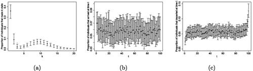
Table 1 Simulation results.

Parameter	N	q11	q12	q01	q02	p1	p2
$\widehat{A}$	505.28	0.02	0.09	0.11	0.29	0.22	0.50
$\widehat{L}$	45.20	0.01	0.01	0.05	0.08	0.06	0.08
cover.	1.00	1.00	1.00	0.80	0.80	0.80	0.80

NOTE: Average over five replications of the posterior mean ( $\widehat{A}$), average width ( $\widehat{L}$) of the 95% PCI and coverage of population size and all cluster-specific parameters.

Hence, our results demonstrate that we can estimate parameters of interest, such as N, and retrieve the latent clustering of the population as well as estimate the corresponding cluster-specific parameters. More details about the simulation study are presented in Section 2.2 of the supplementary materials.

6.2 Angler Data

We fit model of Equation (1)(1) $$\begin{array}{c}N|\nu \sim \text{Poisson}(\Omega )\\ (\mathbf{P}{\mathbf{H}}_1,\mathbf{C}{\mathbf{H}}_1),(\mathbf{P}{\mathbf{H}}_2,\mathbf{C}{\mathbf{H}}_2),\dots ,(\mathbf{P}{\mathbf{H}}_N,\mathbf{C}{\mathbf{H}}_N)|P\\ \hspace{1em}\stackrel{\text{iid}}{\sim }\sum _{c=1}^M\frac{S_c}{\Omega }f(\mathbf{P}{\mathbf{H}}_i,\mathbf{C}{\mathbf{H}}_i|{\tau }_c)\\ P=\sum _{c=1}^M\frac{S_c}{\Omega }{\delta }_{{\tau }_c}\\ M-1\sim \text{Poisson}(\Lambda ),\hspace{1em}{S}_1,\dots ,S_M|M\stackrel{\text{iid}}{\sim }\text{Gamma}(\eta ,\zeta )\\ \mathrm{\hspace{1em}}\mathrm{\hspace{1em}}\text{and}\hspace{1em}{\tau }_1,\dots ,{\tau }_M|M\stackrel{\text{iid}}{\sim }{P}_0,\\ \Lambda \sim \text{Gamma}(a_{\Lambda },b_{\Lambda }),\hspace{1em}\eta \sim \text{Gamma}(a_{\eta },b_{\eta })\\ \mathrm{\hspace{1em}}\mathrm{\hspace{1em}}\text{and}\hspace{1em}\zeta \sim \text{Gamma}(a_{\zeta },b_{\zeta })\end{array}$$(1) to three datasets collected in 2017, 2018, and 2019. We set p = 0 on days when the river was closed for fishing in each season. We adopt an informative approach in the choice of the hyperparmameters of P₀, that is the choice of ${\alpha }_{q_1},{\beta }_{q_1}$, ${\alpha }_{q_0},{\beta }_{q_0}$, and α_p, β_p. Our information can be summarized as follows:

1. an a priori 95% credible interval for the number of visits equal to $[1,12]$, with the lower bound representing individuals who only visit the river once and the upper bound representing individuals who visit on a weekly basis during the season. Since T = 92 here, this gives a (1/92, 12/92) corresponding interval for q₁. Using a set of nonlinear equations, we translated this into a Beta(2.8, 48.7) prior distribution for q₁.

2. an a-priori mean length of stay for an angler equal to 6 days, with a 50% credible interval of roughly [3,7] days. This gives a, roughly, (0.12, 0.26) corresponding interval for q₀, which translates into a Beta(3, 12) prior distribution.

3. a 95% prior credible interval for p equal to (0.1,0.5);

Finally, we assigned vague prior distributions on the parameters Λ, η, and ζ, as described in Section 6.1.

Similarly to the simulation study, we run our algorithm for each dataset using initial adaptive weights equal to 1, h = 0.001 and target acceptance rates equal to 0.2. Convergence was assessed by visual inspection of trace plots and using the Geweke diagnostic in package coda (Plummer et al. 2006), shown in Section 3 of the supplementary materials.

Posterior summaries for N for each year are presented in Table 2. The posterior medians for N are all greater than 3000 and considerably greater than the number of anglers observed each year. There is substantial overlap between all 95% PCIs, suggesting that the population of anglers that visited the river each year between 2017 and 2019 is fairly stable, which is not surprising, as at least 70% of anglers are expected to be returning year after year.

Table 2 Posterior summaries of the population size, N, of anglers for each season.

Year	n	Posterior median	95% PCI
2017	2057	3499	(3208, 3871)
2018	1901	3142	(2857, 3472)
2019	1687	3495	(3036, 3988)

NOTE: The number of anglers observed each season, n, is given in the second column of the table.

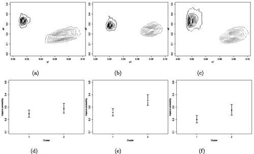
As explained in Section 4, our model induces a clustering amongst anglers, described by our extension of the Chinese restaurant process. We clarify that in this case, the clients are the anglers and the tables are groups of anglers sharing the same characteristics (dishes), with characteristics being the cluster-specific parameters $(q_0,q_1,p)$, which describe the visit behavior and fishing ability of anglers. We summarize the clustering as described in Section 5.4 and obtain two clusters. Contour plots of the posterior distributions for q₀ and q₁ for each cluster and posterior summaries of the cluster-specific probabilities of capture are shown in Figure 5. The largest cluster each year (labelled cluster 1, consisting of 95% of the individuals) is found to consist of the “occasional visitors,” with the lowest q₁ and highest q₀. This group of anglers tend to perform between two and three visits per year, with posterior mean visit duration equal to around two days. The smallest cluster corresponds to the “super-visitors” who make on average around eight visits per year, with posterior mean visit duration between two and three days. We highlight that the estimated capture probability for both clusters, which, although higher for the second cluster is not found to differ significantly between clusters within each season, is considerably greater than what is obtained when a model that does not account for temporary emigration is fitted to the data, as mentioned in Section 2.

Fig. 5 Contour plots of cluster-specific q₀ and q₁ for the 2017, (a), 2018, (b) and 2019, (c), season for cluster 1, solid lines, and cluster 2, dashed lines. Summaries of posterior samples of cluster-specific capture probabilities for the 2017, (d), 2018, (e) and 2019, (f), season.

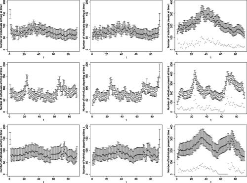
The estimated arrival, departure and presence patterns, presented in Figure 6, vary substantially between years, although a common feature is a larger proportion of individuals estimated to arrive on the first day of the season and similarly to depart on the last day of the season. A peak in the estimated number of individuals present (third column in Figure 6) is observed toward the end of June in all years. This is possibly due to anglers tending to avoid planning a trip to Gaula early in the season as some parts of the river may still be inaccessible due to snow, which is much less likely after the end of June. In 2018 and 2019, there is another peak in the number of anglers present, following river closure at the end of July in both years. We note that, as mentioned above, anglers book their trips typically months in advance, so they tend to remain at the river even when it is closed, waiting for it to reopen once there is sufficient rainfall.

Fig. 6 Posterior medians, indicated by the empty circles, and 95% PCI, indicated by the vertical bars, of the number of individuals arriving (first column), departing (second column), and being present (third column), each day of the season in 2017 (first row), 2018 (second row) and 2019 (third row). The gray dots in the third column indicate the number of anglers who caught at least one salmon that day.

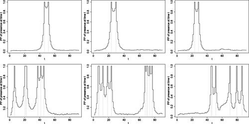
The cluster-specific visit pattern can also be summarized by looking at the posterior probability of presence at any given time point for each individual. In Figure 7 we present these for the most representative individual in each of the two clusters for each year. Individuals representative for each cluster are identified by calculating the distance between each individual and the centroid of each cluster in terms of the number and length of visits and capture probability. The posterior probability of presence is equal to 1 at times when the individual has been observed. This probability decreases as we move away from times of observation. The rate of decrease depends on the cluster and on the number of days between observations. Specifically, the posterior probability of presence reduces slightly more sharply as we move away from the time of observation for individuals in cluster 1 compared to cluster 2. However, even for cluster 1, individuals observed only a few days apart have a high posterior probability of presence between these two observations. As expected, the number of peaks, that is, visits, for each individual corresponds to what we have already identified as typical for each cluster, with individuals in cluster 1 having one or two peaks and individuals in cluster 2 multiple peaks. We focused our interpretation of the clustering results on the individuals observed at least once, since no information, other than the fact that they never caught salmon, is available on the remainder of the individuals. Since our inference on N is performed using a rejection algorithm, the number of individuals that were never observed as well as their corresponding presence histories and hence cluster membership change at every iteration of the algorithm. Therefore, no meaningful posterior summaries exist for particular individuals with index greater than n.

Fig. 7 Posterior probabilities of presence for the most representative individuals in each of the two identified clusters (rows 1 and 2) for 2017 (first column), 2018 (second column) and 2019 (third column).

6.3 The Effect of the COVID-19 Pandemic

In this section, we discuss the results of our model when fitted to the 2020 dataset, presented in Section 3 of the supplementary materials, and compare them to those obtained for the 2017–2019 seasons. In Norway, there were no national travel restrictions in the summer of 2020, so local anglers could still travel to Gaula, but the international travel restrictions meant that the number of anglers traveling from abroad to Norway was dramatically lower. As a result, both the visiting patterns of anglers and their probability of catching salmon whilst at the river were considerably different to pre-pandemic seasons, since the foreign visiting anglers are among the most dedicated and skilled.

We find that we again identify two clusters of anglers, with substantially different visit patterns. The largest cluster, consisting of almost 90% of anglers in the sample, visit one to two times on average in the season. However, the smallest cluster of what we termed “super-visitors” only visit on average around three times in the season, which is considerably lower than in the pre-pandemic seasons. On the other hand, both clusters spent longer at the river per visit on average compared to previous seasons (around six days), which results in average total lengths of stay at the river that are greater than in other seasons (around 15 and 37 days, respectively). Additionally, we estimate that the total number of anglers that visited the river in 2020 was greater than in pre-pandemic seasons (posterior median = 4034, 95% PCI = (3550, 4583)). We note here that once travel restrictions were imposed, the pre-sold fishing licenses where made available to locals in Norway and, given the global travel restrictions, also preventing Norwegians from going on their normal summer vacations, more locals took up the new opportunity to try fishing in Gaula. Finally, our estimated capture probabilities for both clusters are slightly lower than in pre-pandemic seasons (posterior means equal to 0.18 and 0.25, respectively), which is again not surprising as less experienced anglers took the opportunity to visit the river in 2020 compared to the regular and more experienced anglers who usually buy the fishing licenses months in advance.

7 Conclusions

We proposed a novel modeling approach that enables us to estimate parameters of interest, such as the size of a population, from CR data while allowing for temporary emigration and accounting for individual heterogeneity. To our knowledge, this is the only such model for open-populations that does not require the use of methods that rely on Pollock’s robust design, which cannot always be employed, as is the case for the dataset considered in this article.

Our approach brings together CR models, changepoint process and Bayesian nonparametric methodology for the first time and gives rise to a flexible modeling technique for time-series that could be extended to other types of ecological data, such as those collected in occupancy studies (MacKenzie et al. 2002) when the assumption of population closure is not satisfied.

The model is fitted by combining and extending recently-developed algorithms in the area of changepoint processes (Benson and Friel 2018) and a blocked Gibbs sampler for finite mixture models built upon a Bayesian nonparametric approach (Ishwaran and James 2003; Argiento, Bianchini, and Guglielmi 2016; Argiento and De Iorio 2022). The first learn from past states of the MCMC and hence yield proposal distributions that quickly discover the position of changepoints while the latter updates the cluster-specific parameters conditioning on the mixing process P, which yields an independent update (for these parameters) that is more efficient than competing approaches.

We presented a simulation study that demonstrated the reliability of the results obtained by our model and the ability of our method to uncover the underlying clusters in the population as well as to estimate the corresponding cluster-specific parameters. Our analysis of CR datasets on anglers in Norway identified two clusters, each with fairly consistent visit patterns each year, except in 2020, when the effect of the COVID-19 pandemic led to a different angling population. Our results can be used to inform the decisions made by the river management board in terms of number and pricing of fishing licenses issued, based on the quality of fishing in terms of probability to catch a fish on a given day. Reliable estimates of the probability of anglers catching salmon whilst at the river are crucial for effective management of the river and can also be used as a marketing tool by the river management board, as success rates are used as indicators for the quality of fishing experience at rivers. On the other hand, estimates that are biased low, obtained from existing models that do not account for temporary emigration, risk underestimating the effect of angling on the salmon population and cannot guide actions for sustainable fishing at the river.

A natural extension of our model is the inclusion of covariates, for example the effect of rainfall on capture probability throughout the season, to inform estimation about clustering and cluster specific parameters. The use of covariates in mixture models is part of a lively stream of research in the Bayesian nonparametric community (see for instance Foti and Williamson 2013), under the name of (nonexchangeable) dependent processes for mixtures. One of the main advantages of the framework of finite mixture models introduced in Argiento and De Iorio (2022), which we employ in this article, is exactly the possibility of incorporating covariate dependence in the model, and this is a matter of current research. Another interesting extension could consider following the same individuals over different seasons to study the level of consistency in their visiting pattern and the potential improvement of their fishing ability over the years. In 2018, the river closed for the first time in its history because of low levels of rainfall, and since then river closure toward the middle of the season is a recurring phenomenon. As a result, it is expected that anglers will change their behavior about when to book their fishing trip in the future, and our model, or extensions of it described above, could be used to model this behavioral shift.

Acknowledgments

We are grateful to Reinhard Fellner for bringing this case study to our attention, and for all the discussions on the prior knowledge about the system as well as his insights that highlight the importance of our findings and the potential impact of the work presented in this article. We thank the AE and the anonymous referees for all their comments and advice that helped us improve this article.

Supplementary Materials

Title: Supplementary Material Document with three sections: 1. Bayesian mixture model, 2: Posterior characterization, 3: Angler data. The first two give details on the mathematical results of the Bayesian mixture model presented in the article and the algorithm used for inference, with an additional extensive simulation study on prior sensitivity in section 2.2 and the third includes trace plots and diagnostics for all model parameters for the analysis of the data presented in the article.

R code and data: The angler data analyzed in Section 6.2 and the R code used to perform the simulation study and the angler data analysis and to elicit the prior distributions for a number of model parameters in the simulation study presented in the supplementary material.

Disclosure Statement

The authors report there are no competing interests to declare.

References

- Aldous, D. J. (1985), “Exchangeability and Related Topics,” in École d’Été de Probabilités de Saint-Flour XIII–1983, ed. P. L. Hennequin, pp. 1–198, Berlin: Springer.
- Argiento, R., Bianchini, I., and Guglielmi, A. (2016), “Posterior Sampling from ε-Approximation of Normalized Completely Random Measure Mixtures,” Electronic Journal of Statistics, 10, 3516–3547. DOI: 10.1214/16-EJS1168.
- Argiento, R., and De Iorio, M. (2022), “Is Infinity that Far? A Bayesian Nonparametric Perspective of Finite Mixture Models,” Annals of Statistics (to appear).
- Benson, A., and Friel, N. (2018), “Adaptive MCMC for Multiple Changepoint Analysis with Applications to Large Datasets,” Electronic Journal of Statistics, 12, 3365–3396. DOI: 10.1214/18-EJS1418.
- Charalambides, C. A. (2005), Combinatorial Methods in Discrete Distributions (Vol. 600), Hoboken, NJ: Wiley.
- Darroch, J. N. (1958), “The Multiple-Recapture Census: I. Estimation of a Closed Population,” Biometrika, 45, 343–359. DOI: 10.1093/biomet/45.3-4.343.
- Diana, A., Matechou, E., Griffin, J., and Johnston, A. (2020), “A Hierarchical Dependent Dirichlet Process Prior for Modelling Bird Migration Patterns in the UK,” Annals of Applied Statistics, 14, 473–493.
- Favaro, S., and Teh, Y. W. (2013), “MCMC for Normalized Random Measure Mixture Models,” Statistical Science, 28, 335–359. DOI: 10.1214/13-STS422.
- Foti, N. J., and Williamson, S. A. (2013), “A Survey of Non-exchangeable Priors for Bayesian Nonparametric Models,” IEEE Transactions on Pattern Analysis and Machine Intelligence, 37, 359–371. DOI: 10.1109/TPAMI.2013.224.
- Ishwaran, H., and James, L. F. (2003), “Generalized Weighted Chinese Restaurant Processes for Species Sampling Mixture Models,” Statistica Sinica, 13, 1211–1235.
- Jolly, G. M. (1965), “Explicit Estimates from Capture-Recapture Data with both Death and Immigration-Stochastic Model,” Biometrika, 52, 225–247. DOI: 10.1093/biomet/52.1-2.225.
- Kottas, A., and Sansó, B. (2007), “Bayesian Mixture Modeling for Spatial Poisson process Intensities, with Applications to Extreme Value Analysis,” Journal of Statistical Planning and Inference, 137, 3151–3163. DOI: 10.1016/j.jspi.2006.05.022.
- Laake, J. (2013), “RMark: An R Interface for Analysis of Capture-Recapture Data with MARK,” AFSC Processed Rep. 2013-01, Alaska Fish. Sci. Cent., NOAA, Natl. Mar. Fish. Serv., Seattle, WA.
- Lyons, J. E., Kendall, W. L., Royle, J. A., Converse, S. J., Andres, B. A., and Buchanan, J. B. (2016), “Population Size and Stopover Duration Estimation using Mark–Resight Data and Bayesian Analysis of a Superpopulation Model,” Biometrics, 72, 262–271. DOI: 10.1111/biom.12393.
- MacKenzie, D. I., Nichols, J. D., Lachman, G. B., Droege, S., Andrew Royle, J., and Langtimm, C. A. (2002), “Estimating Site Occupancy Rates when Detection Probabilities are less than one,” Ecology, 83, 2248–2255. DOI: 10.1890/0012-9658(2002)083[2248:ESORWD.2.0.CO;2]
- Manrique-Vallier, D. (2016), “Bayesian Population Size Estimation using Dirichlet Process Mixtures,” Biometrics, 72, 1246–1254.
- Matechou, E., and Caron, F. (2017), “Modelling Individual Migration Patterns using a Bayesian Nonparametric Approach for Capture–Recapture Data,” The Annals of Applied Statistics, 11, 21–40. DOI: 10.1214/16-AOAS989.
- Matechou, E., Nicholls, G. K., Morgan, B. J., Collazo, J. A., and Lyons, J. E. (2016), “Bayesian Analysis of Jolly-Seber Type Models,” Environmental and Ecological Statistics, 23, 531–547. DOI: 10.1007/s10651-016-0352-0.
- Miller, J. W., and Harrison, M. T. (2018), “Mixture Models with a Prior on the Number of Components,” Journal of the American Statistical Association, 113, 340–356. DOI: 10.1080/01621459.2016.1255636.
- Molitor, J., Papathomas, M., Jerrett, M., and Richardson, S. (2010), “Bayesian Profile Regression with an Application to the National Survey of Children’s Health,” Biostatistics, 11, 484–498. DOI: 10.1093/biostatistics/kxq013.
- Otis, D. L., Burnham, K. P., White, G. C., and Anderson, D. R. (1978), “Statistical Inference from Capture Data on Closed Animal Populations,” Wildlife Monographs, 62, 3–135.
- Pitman, J. (1996), “Some Developments of the Blackwell-Macqueen urn Scheme,” in Statistics, Probability and Game Theory: Papers in Honor of David Blackwell, volume 30 of IMS Lecture Notes-Monograph Series, eds. T. S. Ferguson, L. S. Shapley, and J. B. MacQueen, pp. 245–267, Hayward, CA: Institute of Mathematical Statistics.
- Pledger, S. (2000), “Unified Maximum Likelihood Estimates for Closed Capture–Recapture Models Using Mixtures,” Biometrics, 56, 434–442. DOI: 10.1111/j.0006-341x.2000.00434.x.
- Pledger, S., Efford, M., Pollock, K., Collazo, J., and Lyons, J. (2009), “Stopover Duration Analysis with Departure Probability Dependent on Unknown Time Since Arrival,” in Modeling Demographic Processes in Marked Populations, eds. D. L. Thomson, E. G. Cooch, and M. J. Conroy, pp. 349–363, New York: Springer.
- Plummer, M., Best, N., Cowles, K., and Vines, K. (2006), “CODA: Convergence Diagnosis and Output Analysis for MCMC,” R News, 6, 7–11.
- Pollock, K. H. (1982), “A Capture-Recapture Design Robust to Unequal Probability of Capture,” The Journal of Wildlife Management, 46, 752–757. DOI: 10.2307/3808568.
- Roberts, G. O., Gelman, A., and Gilks, W. R. (1997), “Weak Convergence and Optimal Scaling of Random Walk Metropolis Algorithms,” Annals of Applied Probability, 7, 110–120.
- Schwarz, C. J., and Arnason, A. N. (1996), “A General Methodology for the Analysis of Capture-Recapture Experiments in Open Populations,” Biometrics, 52, 860–873. DOI: 10.2307/2533048.
- Seber, G. A. F. (1965), “A Note on the Multiple-Recapture Census,” Biometrika, 52, 249–259. DOI: 10.1093/biomet/52.1-2.249.
- Taddy, M. A., and Kottas, A. (2012), “Mixture Modeling for Marked Poisson Processes,” Bayesian Analysis, 7, 335–362. DOI: 10.1214/12-BA711.
- Teh, Y. W., Jordan, M. I., Beal, M. J., and Blei, D. M. (2006), “Hierarchical Dirichlet Processes,” Journal of the American Statistical Association, 101, 1566–1581. DOI: 10.1198/016214506000000302.
- Wade, S., and Ghahramani, Z. (2018), “Bayesian Cluster Analysis: Point Estimation and Credible Balls” (with discussion), Bayesian Analysis, 13, 559–626. DOI: 10.1214/17-BA1073.
- Zhou, M., McCrea, R. S., Matechou, E., Cole, D. J., and Griffiths, R. A. (2019), “Removal Models Accounting for Temporary Emigration,” Biometrics, 75, 24–35. DOI: 10.1111/biom.12961.