On Semiparametrically Dynamic Functional-Coefficient Autoregressive Spatio-Temporal Models with Irregular Location Wide Nonstationarity

Abstract

Nonlinear dynamic modeling of spatio-temporal data is often a challenge, especially due to irregularly observed locations and location-wide nonstationarity. In this article we propose a semiparametric family of Dynamic Functional-coefficient Autoregressive Spatio-Temporal (DyFAST) models to address the difficulties. We specify the autoregressive smoothing coefficients depending dynamically on both a concerned regime and location so that the models can characterize not only the dynamic regime-switching nature but also the location-wide nonstationarity in real data. Different smoothing schemes are then proposed to model the dynamic neighboring-time interaction effects with irregular locations incorporated by (spatial) weight matrices. The first scheme popular in econometrics supposes that the weight matrix is pre-specified. We show that locally optimal bandwidths by a greedy idea popular in machine learning should be cautiously applied. Moreover, many weight matrices can be generated differently by data location features. Model selection is popular, but may suffer from loss of different candidate features. Our second scheme is thus to suggest a weight matrix fusion to let data combine or select the candidates with estimation done simultaneously. Both theoretical properties and Monte Carlo simulations are investigated. The empirical application to an EU energy market dataset further demonstrates the usefulness of our DyFAST models. Supplementary materials for this article are available online.

Keywords:

• Dynamic functional-coefficient autoregression
• Irregular location wide nonstationarity
• Local linear smoothing
• Spatial weight matrix
• Spatio-temporal data

1 Introduction

Nonlinear modeling of complex spatio-temporal processes has been widely recognized an important but challenging issue in analysis of geospatial big data (see Comber and Wulder 2019). In this article we propose a semiparametric family of Dynamic Functional-coefficient Autoregressive Spatio-Temporal (DyFAST) models to address the difficulty in modeling and analysis of our spatio-temporal data, $Y_t(s_i)$, $t=1,\dots ,T$, observed at locations $s_i=(u_i,v_i)$, $i=1,2,\dots ,N$, that are irregularly positioned on the earth surface, with the data nonstationary over the irregular locations in space, where $u_i$ and $v_i$ stand for the latitude and longitude of the location $s_i$. It is well known that time is unidirectional from the past to the future and the popular differencing operation along time hence, makes it easy to change a nonstationary time series into a stationary series (see, Box et al. 2015). However, locations are multidirectional, which makes it harder to turn nonstationary data into stationary ones across locations, in particular with irregularly positioned locations (see, Lu et al. 2009; Al-Sulami et al. 2017). We therefore consider our DyFAST models with such spatio-temporal data that are with irregularly observed locations and location-wide non-stationarity but the data are stationary in the time direction.

The proposed DyFAST models at least own two significant features that make the model family useful. The first feature lies in the autoregressive smoothing coefficients depending both on concerned regime variable and spatial location. They extend linear or semiparametric spatial autoregressive models (see Ord 1975; Gelfand et al. 2003; Hallin, Lu, and Tran 2004; Gao, Lu, and Tjøstheim 2006; Sun et al. 2014, among others) to nonlinear spatio-temporal modeling with irregular locations. Here the dynamic features of spatio-temporal data are characterized by the autoregressive structure together with the advantage of functional (or varying) coefficients (see, e.g., Chen and Tsay 1993; Fan and Zhang 1999). In fact, through the autoregressive smoothing coefficients depending on both regime and location, the DyFAST models not only well characterize the nonlinear dynamic regime-switching nature but also overcome the irregular-location-wide nonstationarity existent in spatio-temporal data.

The second feature of our DyFAST models lies in two schemes proposed to model the dynamic spatial neighboring temporal-lagged effects with the irregular locations by spatial weight matrix. Our first scheme is popular in spatial econometrics with the idea of using spatial weight matrix pre-specified either by experts or by information of spatial locations (see, Anselin 1988). In practice, such spatial weight matrix can be pre-specified in many different ways. Although the idea of model selection can be applied to select an optimal weight matrix among the candidates, it may lead to loss of the important features of different spatial weight matrices (see Zhang and Yu 2018). Our second scheme is therefore to suggest using the idea of weight matrix fusion to combine the candidate spatial weight matrices, letting data decide the significance of each candidate weight matrix. This idea is different from the average of spatial linear AR models with different weight matrices in Zhang and Yu (2018).

Accordingly, different semiparametric estimation procedures for our DyFAST models are suggested. Differently from the two-step estimation procedure (see Lu et al. 2009; Al-Sulami et al. 2017) that separates utilization of spatial and temporal information into two steps, we will first explore a one-step estimation procedure in our Scheme one, where all the data across space and time are used together to estimate the unknown coefficients in one step. Compared with the two-step procedure, we will investigate the differences between both procedures both in theory and in simulation. From the comparisons we will clearly see some advantages of the one-step procedure for data analysis, which will be more identified through simulations. In particular, when the sample sizes are not sufficiently large, we recommend one-step procedure for estimation, while with large sample sizes, we can apply the two-step procedure but should carefully select the bandwidths as done for the one-step one. In fact, we will show that the optimal greedy bandwidths in each step of the two-step procedure would generate poor estimation. Further smoothing estimation procedure by fuzing the spatial weight matrices with Scheme two will be developed on the basis of Scheme one. The large sample theoretical properties and the finite sample Monte Carlo simulations for all the procedures are examined. Our empirical applications to an EU energy market dataset will further illustrate the usefulness of the suggested models and smoothing procedures.

Before ending this section, we should mention that the literatures on spatio-temporal modeling based on linear and/or covariance assumptions are abundant; see Cressie and Wikle (2015) for a comprehensive review and the related references therein. Such linearity assumptions, for many real temporal and spatial data, may actually not be true but an initial or coarse approximation. The nonlinear analyses of time series data have been widely explored in the literature (see, e.g., Tong 1990; Fan and Yao 2003; Gao 2007; Teräsvirta, Tjøstheim, and Granger 2010). However, studies of nonlinear spatio-temporal modeling, in particular with irregular locations, are still rare when compared with the abundant literature of nonlinear time series analysis.

The structure of the remaining of this article is as follows. Section 2 introduces the proposed DyFAST models. Estimation by Scheme one with pre-specified spatial weight matrix is presented in Section 3. Section 4 further develops Scheme two for model estimation with the idea of fusion of spatial weight matrices. Asymptotic properties for the suggested smoothing procedures are developed in those sections. Numerical examples are demonstrated in Section 5 with simulation and Section 6 with real data of retail gasoline prices in European Union countries, both of which illustrate the usefulness of our proposed models and estimation schemes. All technical details together with the related supplementary materials including regularity conditions and proofs for the theorems are provided in an Appendix.

2 Dynamical Functional-Coefficient Autoregressive Spatio-Temporal (DyFAST) Models

We consider a spatio-temporal process $Y_t(s)$ that is observed at discrete time points, $t=1,\dots ,T$ and at irregularly positioned locations, $s_i=(u_i,v_i)$, $i=1,2,\dots ,N$, on a spatial domain $S\subset {\mathbb{R}}^2$, with $u_i$ and $v_i$ being the latitude and longitude of the location $s_i$, respectively. In practice, the data collected are usually nonstationary across space. For example, as indicated in the real data section, Section 6, we will consider the weekly changes of retail gasoline prices over different countries in the EU, which can be seen as stationary along time but nonstationary across different countries of the EU. Here note that different countries are irregularly positioned on the earth surface. We are therefore concerned with how to model the dynamic spatio-temporal lag interactions for this kind of data that are with irregularly observed locations and of location-wide non-stationarity.

To deal with the irregularly observed locations, a popular idea in spatial econometrics (see Anselin 1988) is to model the spatial neighboring effects of $Y_t(s_i)$ by using a spatial weight matrix $W={(w_{ij})}_{N\times N}$, the idea of which can be traced back to Cliff and Ord (1972) and Ord (1975), to define a so-called spatial lag (SL) variable(2.1) $$Y_t^{\text{SL}}(s_i)={\sum }_{j=1}^N{w}_{ij}{Y}_t(s_j),$$(2.1) where W is a row-wise standardized $N\times N$ matrix, with its elements $w_{ij}$ satisfying $w_{ij}\ge 0$, ${\sum }_{j=1}^N{w}_{ij}=1$ and $w_{ii}=0$. This pre-specified spatial weight matrix W can be presented either by experts’ knowledge or by using location-related information (see Anselin 1988, chap. 3). Often, the elements $w_{ij}$’s are specified as a continuous function of $s_i$, say, the inverse of the distance between $s_i$ and $s_j$, except at $s_i=s_j$, for which $w_{ii}=0$. Here $Y_t(s_i)$ is allowed to be of the so-called nugget effect involved in $Z_t(s_i)$ (see, (3.2) in Section 3 and Assumption (A3)(iv) in Appendix A.1).

The idea of our proposed family of DyFAST models comes from taking into account the dynamic autoregressive impacts on $Y_t(s)$ from both the spatial neighboring lags and the temporal lags of $Y_t(s)$, the coefficients of which not only depend on the location s but also vary with a regime-switching covariate variable $X_t(s)$, either a temporal or spatio-temporal process that is observable. In applications, this $X_t(s)$ may either be exogenous or some temporal lag of $Y_t(s)$ that is of some real meaning. Then our semiparametric class of DyFAST models can be defined in the form(2.2) $$\begin{array}{cc}{Y}_t(s_i)={\beta }_0(X_t(s_i),s_i)+{\sum }_{j=1}^p{\beta }_j(X_t(s_i),s_i)Y_{t-j}^{\text{SL}}(s_i)\hfill & \hfill \\ \hspace{1em}+{\sum }_{l=1}^q{\beta }_{p+l}(X_t(s_i),s_i)Y_{t-l}(s_i)\hfill & \hfill \\ \hspace{1em}+{\epsilon }_t(s_i),\hspace{1em}i=1,\dots ,N,t=r+1,\dots ,T,\hfill & \hfill \end{array}$$(2.2) where p and q are the neighboring and the location itself autoregressive lag orders, respectively, with $r=\max \{p,q\}$, and the autoregressive coefficients, ${\beta }_j(\cdot ,\cdot )$, $j=0,1,\dots ,p+q$, are unknown functional of the regime variable $X_t(s_i)$ and location $s_i$, to characterize the nonlinear dynamic behavior and location-wise nonstationarity of $Y_t(s_i)$, with ${\beta }_0(\cdot ,\cdot )$ for intercept, ${\beta }_j(\cdot ,\cdot )$, $j=1,\dots ,p$, for spatial neighboring time-lag interactions, and ${\beta }_j(\cdot ,\cdot )$, $j=p+1,\dots ,p+q$, for time-lag effects of $Y_t(s_i)$ itself, and ${\epsilon }_t(s_i)$ is the error process of the model.

This semiparametric family takes account of some salient features of dynamic spatio-temporal data. It covers a wide range of existent models in the literature. For example, it extends, to the spatio-temporal network setting, the nonlinear functional-coefficient autoregressive time series model at each fixed location $s_i$, which is very popular in the literature of time series data analysis (see Chen and Tsay 1993; Cai, Fan, and Yao 2000). Our DyFAST family also extends the semiparametric spatio-temporal models of Subba Rao (2008), Lu et al. (2009), and Al-Sulami et al. (2017), among others. For example, when ${\beta }_j(\cdot ,\cdot )$, $j=1,\dots ,p+q$, are independent of the regime variable $X_t(s_i)$, the DyFAST models reduce to a linear or partially linear spatio-temporal autoregressive model from the forecasting perspective (see Al-Sulami et al. 2017). This kind of autoregressive spatio-temporal model can hence well characterize the location-wise nonstationarity existent in the data. However, at each location $s_i$, it is still a constant coefficient linear time series model. In fact, Subba Rao (2008) only considered the temporal lag effect without taking the spatial neighboring effects into account, while Lu et al. (2009) only applies to the case when the data are observed regularly on a lattice with a small same number of neighboring variables able to be well specified for each site, which is impossible to be implemented for irregularly positioned data considered in this article. Furthermore, the considered model of Al-Sulami et al. (2017) is only a special case of model (2.2) as mentioned, which is unable to capture the dynamic regime-switching effects in reality. Clearly, our DyFAST model (2.2) can overcome these shortcomings.

We will propose two schemes to estimate the dynamic spatial neighboring temporal-lagged effects in model (2.2) adapting to the irregular locations. Our first scheme uses the idea of spatial weight matrix pre-specified either by experts or by the prior information of spatial locations. Because such a spatial weight matrix may be pre-specified in many different ways (see, Anselin 1988), our second scheme is to propose an idea of combining the candidate spatial weight matrices, letting data decide the significance of each candidate. Accordingly, we will suggest different semiparametric estimation procedures detailed below.

3 Scheme 1: Pre-specified Spatial Weight Matrix

With a pre-specified spatial weight matrix W given, the DyFAST models given in (2.2) can be rewritten as(3.1) $$Y_t(s_i)=Z_t{(s_i)}^{\prime }\beta (X_t(s_i),s_i)+{\epsilon }_t(s_i),$$(3.1) for $t=r+1,\dots ,T$, with $r=\max \{p,q\}$, and $i=1,\dots ,N$, where the notation $A^{\prime }$ denotes the transpose of a vector or matrix A,(3.2) $$Z_t(s_i)={(1,Y_{t-1}^{\text{SL}}(s_i),\dots ,Y_{t-p}^{\text{SL}}(s_i),Y_{t-1}(s_i),\dots ,Y_{t-q}(s_i))}^{\prime },$$(3.2) the vector of spatio-temporally lagged variables, and(3.3) $$\begin{array}{cc}\beta (x,s)=({\beta }_0(x,s),{\beta }_1(x,s),\dots ,{\beta }_p(x,s),{\beta }_{p+1}(x,s),\dots ,\hfill & \hfill \\ \hspace{1em}{\beta }_{p+q}(x,s){)}^{\prime },\hfill & \hfill \end{array}$$(3.3) the corresponding vector of functional autoregressive coefficients.

3.1 A One-Step Estimation Method

We first consider to estimate the coefficients $\beta (\cdot ,\cdot )$ in (3.1). Differently from the two-step estimation procedure (see, Lu et al. 2009; Al-Sulami et al. 2017) separating utilization of spatial and temporal information into two steps, this study suggests a one-step estimation procedure by considering ${\beta }_j(X_t(s_i),s_i)$ as a function of $X_t(s_i)$ and $s_i$. In this procedure, all the data across space and time are used together to estimate the coefficients $\beta (\cdot ,\cdot )$ in one step.

By the idea of local linear fitting (see Fan and Gijbels 1996), we can approximate the unknown function ${\beta }_j(X_t(s_i),s_i)$ by a local linear function if $(X_t(s_i),s_i)$ is close to $(x,s)$. For a given $s={(u,v)}^{\prime }$, we denote ${(\partial \beta (x,s)/\partial u,\partial \beta (x,s)/\partial v)}^{\prime }$ by ${\dot{\beta }}^s(x,s)$ and $\partial \beta (x,s)/\partial x$ by ${\dot{\beta }}^x(x,s)$, where$$\partial \beta (x,s)/\partial u={\left(\partial {\beta }_0(x,s)/\partial u,\dots ,\partial {\beta }_{p+q}(x,s)/\partial u\right)}^{\prime }$$

and $\partial \beta (x,s)/\partial v$ is defined similarly. Then for any $X_t(s_i)$ and $s_i$ in the neighborhood of x and s, respectively, we have(3.4) $$\begin{array}{cc}{\beta }_j(X_t(s_i),s_i)\approx {\beta }_j(x,s)+{\dot{\beta }}_j^x(x,s)(X_t(s_i)-x)+{\dot{\beta }}_j^s{(x,s)}^{\prime }(s_i-s)\hfill & \hfill \\ =:b_{0,j}+b_{1,j}(X_t(s_i)-x)\hfill & \hfill \\ \hspace{1em}+b_{2,j}^{\prime }(s_i-s),j=0,1,2,\dots ,p+q.\hfill & \hfill \end{array}$$(3.4)

Locally, estimating $(\beta (x,s), {\dot{\beta }}^x(x,s), {\dot{\beta }}^s{(x,s)}^{\prime })$ is equivalent to estimating $(b_0, b_1, b_2^{\prime })$, where $b_k={(b_{k,0},b_{k,1},\dots ,b_{k,(p+q)})}^{\prime }$ for $k=0,1,2$. This motivates an estimator by setting ${\widehat{\beta }}_j(x,s)=:{\widehat{b}}_{0,j}$, $\widehat{{\dot{\beta }}_j^x}(x,s)=:{\widehat{b}}_{1,j}$, and $\widehat{{\dot{\beta }}_j^s}(x,s)=:{\widehat{b}}_{2,j}$, minimizing(3.5) $$\begin{array}{c}{\sum }_{i=1}^N{\sum }_{t=r+1}^T[Y_t(s_i)-{\sum }_{j=0}^{p+q}\{b_{0,j}+b_{1,j}(X_t(s_i)-x)\\ \hspace{1em}+{b^{\prime }}_{2,j}(s_i-s)\}{Z}_{t,j}(s_i){]}^2{K}_{it},\end{array}$$(3.5) with respect to $b_k={(b_{k,0},b_{k,1},\dots ,b_{k,(p+q)})}^{\prime }$, $k=0,1,2$, where $K_{it}=K_{h_1}(X_t(s_i)-x)L_{h_2}(s_i-s),$ $K_{h_1}(x)=h_1^{-1}K(x/h_1)$, with K a kernel function on ${\mathbb{R}}^1$ and $h_1>0$ a bandwidth, and $L_{h_2}(s)=h_2^{-2}L(s/h_2)$ with L a kernel function on ${\mathbb{R}}^2$ and $h_2>0$ another bandwidth.

We let $Y = {(Y_{r+1}(s_1),\dots ,Y_T(s_1),\dots ,Y_{r+1}(s_N),\dots ,Y_T(s_N))}^{\prime }$ denote a $N{T}_0$-dimensional vector, with $T_0=T-r$. Also, denote by $\otimes$ the Kronecker product and ${\mathbf{1}}_{p+q+1}={(1,1,\dots ,1)}^{\prime }$ the $(p+q+1)$-dimensional vector with all components being 1. Then, with $e_1=(1,0,0,0)\otimes \text{diag}({\mathbf{1}}_{p+q+1}^{\prime })$, the local linear estimator of $\beta (x,s)$ derived from (3.5) is given by(3.6) $$\widehat{\beta }(x,s)={\widehat{b}}_0=e_1{U}_{TN}^{-1}{V}_{TN},$$(3.6) where $U_{TN}={(N{T}_0)}^{-1}{\tilde{Z}}^{\prime }\tilde{W}\tilde{Z}$ and $V_{TN}={(N{T}_0)}^{-1}{\tilde{Z}}^{\prime }\tilde{W}Y,$ with $\tilde{Z}$ denoting an $N{T}_0\times 4(p+q+1)$ matrix with its $(i\times T_0+t-r)$ th row equal to$$\left(Z_t{(s_i)}^{\prime },\{(X_t(s_i)-x)/h_1\}{Z}_t{(s_i)}^{\prime },{(\{(s_i-s)/h_2\}\otimes Z_t(s_i))}^{\prime }\right)$$

for $i=1,\dots ,N$ and $t=r+1,\dots ,T$, and$$\begin{array}{cc}\mathrm{ }\tilde{W}=\text{diag}\{K_h(X_{r+1}(s_1)-x)L_h(s_1-s),\dots ,\hfill & \hfill \\ \hspace{1em}{K}_h(X_T(s_1)-x)L_h(s_1-s),\dots ,\hfill & \hfill \\ \hspace{1em}{K}_h(X_{r+1}(s_N)-x)L_h(s_N-s),\dots ,\hfill & \hfill \\ \hspace{1em}{K}_h(X_T(s_N)-x)L_h(s_N-s)\}.\hfill & \hfill \end{array}$$

3.2 Asymptotic Property

We establish the asymptotic property for the estimator $\widehat{\beta }(x,s)$ in this section. All the regularity assumptions needed are collected in Appendix A.1. Let $H_{it}={(1,\frac{X_t(s_i)-x}{h_1},{(\frac{s_i-s}{h_2})}^{\prime })}^{\prime }$. Then it follows from (3.6) that(3.7) $$\begin{array}{cc}{U}_{TN}\hfill & ={(T_{0}N)}^{-1}{\sum }_{i=1}^N{\sum }_{t=r+1}^T{H}_{it}{H}_{it}^{\prime }\otimes Z_t(s_i)Z_t{(s_i)}^{\prime }{K}_{it},\hfill \end{array}$$(3.7) (3.8) $$V_{TN}={(T_{0}N)}^{-1}{\sum }_{i=1}^N{\sum }_{t=r+1}^T{H}_{it}\otimes Z_t(s_i)Y_t(s_i)K_{it}.$$(3.8)

Then by (3.6) together with (3.7) and (3.8), we have(3.9) $$\left(\widehat{\beta }(x,s)-\beta (x,s)\right)=\left({\widehat{b}}_0-b_0\right)=e_1{U}_{TN}^{-1}{\mathcal{W}}_{TN},$$(3.9) (3.10) $${\mathcal{W}}_{TN}:={(T_{0}N)}^{-1}{\sum }_{i=1}^N{\sum }_{t=r+1}^T(H_{it})\otimes Y_t^{*}(s_i)Z_t(s_i)K_{it},$$(3.10) where $Y_t^{*}(s_i):=Y_t(s_i)-{[b_0+b_1(X_t(s_i)-x)+b_2^{\prime }(s_i-s)]}^{\prime }{Z}_t(s_i)$.

We give some preliminary lemmas before stating the asymptotic normality for $\widehat{\beta }(x,s)$. We need to introduce some additional notations. Denote by $f_X(x,s)$ the marginal probability density function of $X_t(s)$ at a given location s, $f_S(s)$ the intensity function of the observing locations $\left\{s_i\right\}$, $\Omega (x,s)=E[Z_t(s)Z_t{(s)}^{\prime }|X_t(s)=x]$, and ${\mu }_2^K=\int u^{2}K(u)du$, ${\mu }_2^L=\int u{u}^{\prime }L(u)du$.

Lemma 3.1

.

Under the assumptions given in Appendix A.1,$$U_{TN}\stackrel{\mathrm{P}}{\to }U:=f_X(x,s)f_S(s)\left(\begin{array}{ccc}\Omega (x,s)& 0& 0\\ 0& \Omega (x,s){\mu }_2^K& 0\\ 0& 0& {\mu }_2^L\otimes \Omega (x,s)\end{array}\right)$$as $T_0,N\to \infty$, where $\stackrel{\mathrm{P}}{\to }$ stands for convergence in probability.

Next, we consider the asymptotic behavior of ${\mathcal{W}}_{TN}$, with its components ${\mathcal{W}}_{TN,j}$, for $j=1,2,3$, corresponding to those of $H_{it}$ in (3.10), respectively.

Lemma 3.2

.

Under the assumptions given in Appendix A.1,(3.11) $$\mathrm{E}\left[{\mathcal{W}}_{TN,1}\right]=f_X(x,s)f_S(s)\Omega (x,s)B_0(x,s)+o\left(h_1^2+h_2^2\right),$$(3.11) $$\mathrm{E}\left[{\mathcal{W}}_{TN,j}\right]=o\left(h_1^2+h_2^2\right),\hspace{1em}j=2,3$$as $T_0,N\to \infty$, where $B_0(x,s)=(h_1^2/2){\mu }_1(x,s)+(h_2^2/2){\mu }_2(x,s)$, with$$\begin{array}{c}{\mu }_1(x,s)=({\partial }^2\beta (x,s)/\partial x^2)\int u^{2}K(u)du,\\ {\mu }_2(x,s)={({\mu }_{2,0},\dots ,{\mu }_{2,p+q})}^{\prime },\text{\hspace{0.17em}with}\\ {\mu }_{2,j}=\text{tr}\left\{({\partial }^2{\beta }_j(x,s)/\partial s\partial s^{\prime })\int z{z}^{\prime }L(z)dz\right\}.\end{array}$$

The following lemma provides the asymptotic variance of ${\mathcal{W}}_{TN,1}$.

Lemma 3.3

.

Under the assumptions in Appendix A.1,(3.12) $$\begin{array}{cc}\text{var}\left[{\mathcal{W}}_{TN,1}\right]={\left(T_0{h}_{1}N{h}_2{}^2\right)}^{-1}{\Sigma }_1(1+o(1))\hfill & \hfill \\ \hspace{1em}+T_0^{-1}{\Sigma }_2(1+o(1)),\hfill & \hfill \end{array}$$(3.12) where$$\begin{array}{cc}{\Sigma }_1={\sigma }^2(s)\Omega (x,s)f_S(s)f_X(x;s)\int K^2(u)du\int L^2(z)dz,\hfill & \hfill \\ {\Sigma }_2=\Gamma (x;s,s){\Omega }^{*}(x;s,s)f_S^2(s)q(x,x;s).\hfill & \hfill \end{array}$$

Here ${\sigma }^2(s)=\text{var}({\epsilon }_1(s))$, $\Gamma (x;s,s)$ and ${\Omega }^{*}(x;s,s)$ are the limits of $\Gamma (x;s_i,s_j)=\mathrm{E}({\epsilon }_t(s_i){\epsilon }_t(s_j)|X_t(s_i)=x,X_t(s_j)=x)$ and ${\Omega }^{*}(x,s_i,s_j)=E[Z_t(s_i)Z_t{(s_j)}^{\prime }|X_t(s_i)=x,X_t(s_j)=x]$, respectively, and $q(x,y;s)$ is the limit of the joint probability density $p(x,y;s_i,s_j)$ of $(X_t(s_i),X_t(s_j))$, defined in Assumption (A1), as $s_i$ and $s_j$ tend to s (i.e., $\Vert s_i-s\Vert \to 0$ and $\Vert s_i-s\Vert \to 0$ with $\Vert \cdot \Vert$ for the Euclidean norm in $R^2$).

We remark that the notations $\Gamma (x;s,s)$, ${\Omega }^{*}(x;s,s)$ and $q(x,y;s)$ given in ${\Sigma }_2$ in Lemma 3.3 are denoted simply for the limits of $\Gamma (x;s_i,s_j)$, ${\Omega }^{*}(x,s_i,s_j)$ and $p(x,y;s_i,s_j)$ as $s_i$ and $s_j$ tend to s. They do not mean that $\Gamma (x;s_i,s_j)$, ${\Omega }^{*}(x,s_i,s_j)$ and $p(x,y;s_i,s_j)$ are continuous at $(s_i,s_j)=(s,s)$, which may not hold true in the presence of the so-called nugget effect (Cressie 1993, sec. 2.3.1). See also the discussions in Lu, Tjøstheim, and Yao (2008) and Lu et al. (2009).

We now present the asymptotic normality result.

Theorem 3.1

.

Let the Assumptions in Appendix A.1 hold. Then(3.13) $$\begin{array}{cc}\widehat{\beta }(x,s)-\beta (x,s)=B_0(x,s)+o(h_1^2+h_2^2)\hfill & \hfill \\ +\left\{{\left(T_0{h}_{1}N{h}_2{}^2\right)}^{-\frac{1}{2}}{\Theta }_1+T_0^{-\frac{1}{2}}{\Theta }_2\right\}\eta (s)(1+o_p(1)),\hfill & \hfill \end{array}$$(3.13) as $T_0,N\to \infty$, where $B_0(x,s)$ is defined in Lemma 3.2, $\eta (s)$ is a $(p+q+1)$-dimensional normal random vector with zero mean and identity variance matrix, and ${\Theta }_1$ and ${\Theta }_2$ are two $(p+q+1)\times (p+q+1)$ matrices, satisfying$$\begin{array}{cc}{\Theta }_1{\Theta }_1^{\prime }={\sigma }^2(s)\{{\Omega }^{-1}(x,s)/(f_S(s)f_X(x;s))\}\int K^2(u)du\int L^2(z)dz,\hfill & \hfill \\ {\Theta }_2{\Theta }_2^{\prime }=\Gamma (x;s,s)\{{\Omega }^{-1}(x,s){\Omega }^{*}(x,s,s){\Omega }^{-1}(x,s)/f_X^2(x,s)\}q(x,x;s).\hfill & \hfill \end{array}$$

The proof of the lemmas and Theorem 3.1 will be given in Appendix A.3.

Remark 1.

From Theorem 3.1, the optimal bandwidths for estimating ${\beta }_j(x,s)$ in the one-step method can be obtained by minimizing the asymptotic mean squared error of the estimator in the form(3.14) $$\left[{\left(c_2{h}_1^2+c_3{h}_2^2\right)}^2+c_4/\left\{T_{0}N{h}_1{h}_2^2\right\}\right],$$(3.14) minimizing of which with respect to $(h_1,h_2)$ leads to the optimal bandwidths(3.15) $$\begin{array}{cc}{h}_1={\left((c_3{c}_4)/\left\{4c_2^2{T}_{0}N\right\}\right)}^{1/7},\hfill & \hfill \\ h_2={\left(\left\{2^{3/2}{c}_2^{3/2}{c}_4\right\}/\left\{c_3^{5/2}{T}_{0}N\right\}\right)}^{1/7},\hfill & \hfill \end{array}$$(3.15) where $c_2=\frac{1}{2}\frac{{\partial }^2{\beta }_j(x,s)}{\partial x^2}\int u^{2}K(u)du$, $c_3=\frac{1}{2}\mathrm{tr}\{{\partial }^2{\beta }_j(x,s)/\partial s\partial s^{\prime }\int z{z}^{\prime }L(z)dz\}$, and$$c_4=\left(\{{\sigma }^2(s)e_j^{\prime }{\Omega }^{-1}(x,s)e_j\}/\{f_X(x;s)f_S(s)\}\right)\int K^2(u)du\int L^2(u)du.$$

Remark 2.

Based on the optimal bandwidths as given in Remark 1, we have $h_{1}N{h}_2^2=O(N/{(T_{0}N)}^{3/7})=O({(N^4/T_0^3)}^{1/7})$. Therefore, if $\underset{N,T\to \infty }{\lim }{h}_{1}N{h}_2{}^2=\underset{N,T\to \infty }{\lim }O({(N^4/T_0^3)}^{1/7})=0$, then the rate of the convergence for $\widehat{\beta }(x,s)$ is of the usual semiparametric order ${(T_0{h}_{1}N{h}_2{}^2)}^{\frac{1}{2}}=o\left(T_0^{\frac{1}{2}}\right)$ on the left hand side of (3.13). Alternatively, if $\underset{N,T\to \infty }{\lim }{h}_{1}N{h}_2{}^2=\underset{N,T\to \infty }{\lim }O({(N^4/T_0^3)}^{1/7})>0$, then the rate of the convergence for $\widehat{\beta }(x,s)$ is of order $T^{\frac{1}{2}}$ on the left hand side of (3.13). This implies that if the observing (spatial) locations are sufficiently dense with the number N sufficiently large relatively to the time series sample size T, our semiparametric estimator can even achieve the time series parametric rate of root T (up to the bias), which is an interesting finding with modeling of spatio-temporal data by the one-step procedure.

3.3 Discussion on Comparison with a Two-Step Procedure

Alternative to the above estimation, we can develop a two-step procedure for estimating the unknown function $\beta (\cdot ,\cdot )$ as in Lu et al. (2009) and Al-Sulami et al. (2017), which is sketched for comparison as follows.

Step 1: (Time-series based estimation) This step just follows the estimation procedure in Cai, Fan, and Yao (2000). For each location $s_i$, the functions ${\beta }_j(X_t(s_i),s_i)$ are estimated by a local linear fitting. For $X_t(s_i)$ in the neighborhood of x,(3.16) $$\begin{array}{cc}{\beta }_j(X_t(s_i),s_i)\approx {\beta }_j(x,s_i)+{\dot{\beta }}_j(x,s_i)(X_t(s_i)-x)\hfill & \hfill \\ =:a_j+b_j(X_t(s_i)-x).\hfill & \hfill \end{array}$$(3.16)

Then, we define an estimator by ${\widehat{\beta }}_j(x,s_i)=:{\widehat{a}}_j$ and $\widehat{{\dot{\beta }}_j}(x,s_i)=:{\widehat{b}}_j$, minimizing(3.17) $$\begin{array}{c}{\sum }_{t=r+1}^T{\left[Y_t(s_i)-{\sum }_{j=0}^{p+q}\left\{a_j+b_j(X_t(s_i)-x)\right\}{Z}_{t,j}(s_i)\right]}^2\\ K_{h_1}(X_t(s_i)-x),\end{array}$$(3.17) w.r.t. $a_j,b_j,j=0,1,\dots ,p+q$, where $K_{h_1}(x)=h_1^{-1}K(x/h_1)$, with K the kernel function on ${\mathbb{R}}^1$ and $h_1>0$ denoting the temporal bandwidth.

Then the local linear estimators can be expressed as(3.18) $$\widehat{\beta }(x,s_i)=\overline{e}{(A_i{(x)}^{\prime }{B}_i(x)A_i(x))}^{-1}{A}_i{(x)}^{\prime }{B}_i(x)Y(s_i),$$(3.18)

where $\overline{e}=(1,0)\otimes \text{diag}({\mathbf{1}}_{p+q+1})$, $A_i(x)$ denotes an $T_0\times 2(p+q+1)$ matrix with $(Z_t{(s_i)}^{\prime },(X_t(s_i)-x)Z_t{(s_i)}^{\prime })$ as its $t-r$ th row for $t=r+1,\dots ,T$, and$$\begin{array}{cc}{B}_i(x)=\hfill & \text{diag}\{K_{h_1}(X_{r+1}(s_i)-x),\dots ,K_{h_1}(X_T(s_i)-x)\}.\hfill \end{array}$$

Step 2: (Spatial smoothing) The estimators based on Step-1 procedure can be improved by pooling the information from neighboring locations by spatial smoothing (Lu et al. 2009). At the observing locations $\{s_i,i=1,2,\dots ,N\}\subset S$, there is a spatial sampling intensity function $f_S$ over S (see Assumptions in Appendix A.1). Then a spatial smoothing estimator of $\beta (x,s)$ is obtained by(3.19) $${\tilde{\beta }}_j(x,s)={\sum }_{i=1}^N{\tilde{L}}_{h_2,i}^{*}\left(s\right){\widehat{\beta }}_j(x,s_i),j=0,1,2,\dots ,p+q,$$(3.19) where ${\tilde{L}}_{h_2,i}^{*}(s)$ is the ith component of ${\tilde{e}}_1^{\prime }{(C^{\prime }DC)}^{-1}{C}^{\prime }D$, a local linear fitting equivalent kernel function on ${\mathbb{R}}^2$. Here ${\tilde{e}}_1={(1,0,0)}^{\prime }\in {\mathbb{R}}^3$, $C=C(s)$ denotes an $N\times 3$ matrix with the ith-row $(1,{(s_i-s)}^{\prime }/h_2)$, and $D=D(s)=\text{diag}{\left\{L_{h_2}(s_i-s)\right\}}_{i=1}^N$ with $L_{h_2}(\cdot )=L(\cdot /h_2)/h_2^{-2}$ and $L(\cdot )$ a kernel on ${\mathbb{R}}^2$.

Theorem 3.2

.

Under Assumptions in Appendix A.1, as $T_0,N\to \infty$, the Step 1 estimator satisfies that for $s_i\in S$,(3.20) $$\begin{array}{cc}\widehat{\beta }(x,s_i)-\beta (x,s_i)=\frac{h_1^2}{2}{\mu }_1(x,s_i)+o(h_1^2)\hfill & \hfill \\ \hspace{1em}+\left\{{\left(T_0{h}_1\right)}^{-\frac{1}{2}}{\Theta }_1(s_i)\right\}\eta (s_i)(1+o_p(1)),\hfill & \hfill \end{array}$$(3.20) and the Step 2 estimator satisfies that for $s\in S$,(3.21) $$\begin{array}{cc}\tilde{\beta }(x,s)-\beta (x,s)=\frac{h_1^2}{2}{\mu }_1(x,s)+\frac{h_2^2}{2}{\mu }_2(x,s)+o(h_1^2+h_2^2)\hfill & \hfill \\ +\left\{{\left(T_0{h}_{1}N{h}_2{}^2\right)}^{-\frac{1}{2}}{\Theta }_1+T_0^{-\frac{1}{2}}{\Theta }_2\right\}\eta (s)(1+o_p(1)),\hfill & \hfill \end{array}$$(3.21) where $\eta (s)$ is a $(p+q+1)$ random vector with zero mean and identity variance matrix, with ${\mu }_1(x,s)$, ${\mu }_2(x,s)$ and ${\Theta }_1={\Theta }_1(s)$ and ${\Theta }_2={\Theta }_2(s)$ as defined in Theorem 3.1.

Remark 3

.

The optimal greedy bandwidth $h_1$ for time series based estimation at each location $s_i$ is derived similarly to that of Cai, Fan, and Yao (2000), which is $h_1=O(T_0^{-1/5})$ following from (3.20). Here “greedy” means that the bandwidths are chosen to be optimal locally stepwise at all the locations, respectively, a popular idea applied in machine learning modeling. Then, with this order of $h_1$, by minimizing the squared bias plus variance of $\tilde{\beta }(x,s)$ given in (3.21), we can find $h_2=O({(N{h}_1{T}_0)}^{-1/6})$ for the two-step procedure (note that this differs from the standard optimal bandwidth for spatial smoothing that is of order $O(N^{-1/6})$ in view of the two-dimensional smoothing). Clearly these $h_1$ and $h_2$ are different from those optimal bandwidths in (3.15) for the one-step estimation procedure given in Theorem 3.1.

Remark 4

.

It is interesting to discuss the comparison between the one-step and the two-step procedures. We note from (3.13) in Theorem 3.1 and (3.21) in Theorem 3.2 that the one-step and two-step methods have the same form of asymptotic biases and variances so they have the same form of Asymptotic Mean Squared Estimation Error (AMSE) as given in (3.14) in Remark 1. However, for the two-step estimation with the optimal bandwidths $h_1=O(T_0^{-1/5})$ in Step 1 and $h_2=O({(N{T}_0{h}_1)}^{-1/6})=O({(N{T}_0^{4/5})}^{-1/6})$ in Step 2 (or even worse if $h_2=O(N^{-1/6})$), it leads to, from (3.14), that(3.22) $$\begin{array}{cc}{\text{AMSE}}^{\text{two}}=[{\left(O(T_0^{-2/5})+O\left({(N{T}_0^{4/5})}^{-2/6}\right)\right)}^2\hfill & \hfill \\ \hspace{1em}+\frac{O(1)}{T_{0}N(T_0^{-1/5})\left({(N{T}_0^{4/5})}^{-2/6}\right)}]\hfill & \hfill \\ =O(\left(T_0^{-4/5}\right)+\left(T_0^{-2/3}{N}^{-1/3}\right)\hfill & \hfill \\ \hspace{1em}+\left(T_0^{-8/15}{N}^{-2/3}\right)+\left(T_0^{-4/15}{N}^{-2/3}\right)),\hfill & \hfill \end{array}$$(3.22) while for the one-step procedure with the optimal bandwidths $h_1$ and $h_2$ given in (3.15), it leads to, from (3.14), that(3.23) $${\text{AMSE}}^{\text{one}}=O\left({(T_{0}N)}^{-4/7}\right).$$(3.23)

Remark 5

.

Clearly ${\text{AMSE}}^{\text{two}}$ in (3.22) is much larger than ${\text{AMSE}}^{\text{one}}$ in (3.23). In fact it follows from (3.22) and (3.23) that(3.24) $$\begin{array}{cc}\frac{{\text{AMSE}}^{\text{two}}}{{\text{AMSE}}^{\text{one}}}=O(\left(T_0^{-\frac{8}{35}}{N}^{\frac{4}{7}}\right)+\left(T_0^{-\frac{2}{21}}{N}^{\frac{5}{21}}\right)\hfill & \hfill \\ \hspace{1em}+\left(N^{-\frac{2}{21}}{T}_0^{4/105}\right)+\left(T_0^{\frac{32}{105}}{N}^{-\frac{2}{21}}\right)).\hfill & \hfill \end{array}$$(3.24)

For example, consider the summation of the first and fourth terms on the RHS of (3.24), the minimum of which is achieved and equal to $O(T_0^{8/35})\to \infty$ when $T_0^{-\frac{8}{35}}{N}^{\frac{4}{7}}=T_0^{\frac{32}{105}}{N}^{-\frac{2}{21}}$, that is, $N=T_0^{4/5}$. Therefore, (3.24) actually tends to infinity as $T,N\to \infty$. This implies that the usual two-step estimation procedure with optimal greedy bandwidths in each of the two steps is not an optimal estimation. See more comparison of both methods in Section 5.

From Theorems 3.1 and 3.2 and the discussions above, we may conclude that when the sample sizes tend to infinity, both procedures of one-step and two-step share the same asymptotic mean squared errors. However, when applying the two-step procedure, the optimal greedy (i.e., locally optimal) bandwidths would generate poor estimation. In particular, when the sample sizes are not sufficiently large, we recommend one-step procedure for estimation, while with large sample sizes, we can apply the two-step procedure but should carefully select the bandwidths as done for the one-step one (see Section A.2).

4 Scheme 2: Fusion of Spatial Weight Matrices

In Section 3, we assume the spatial weight matrix W is well pre-specified. In real applications, it may not be always the case, and one can often specify different spatial weight matrices based on different features of the real data, such as distance based spatial weight matrix $W_1$ or contiguity based spatial weight matrix $W_2$, and so on (see, Anselin 1988). A significant problem is how those spatial weight matrices should be used for modeling in applications. We suggest a weight matrix fusion idea to solve the issue.

For simplicity, let us look at two spatial weight matrices $W_1$ and $W_2$ (the case for more than two spatial weight matrices is easily extended), which we suppose are well pre-specified and linearly independent so that both weight matrices are essentially different, for model identifiability. We consider a convenient fusion idea of combining different individual spatial weight matrices in a form(4.1) $$W=a_1{W}_1+a_2{W}_2,$$(4.1) where $a_1$ and $a_2$ are unknown constants satisfying $a_1+a_2=1$ so that W is row-wise standardized if $W_1$ and $W_2$ are row-wise standardized. Here we do not suppose $a_k$’s are necessarily nonnegative. So the elements of our new W may be negative and W is a kind of generalized spatial weight matrix. We let the data decide the combining weights $a_k$. Therefore, we have here extended model (2.2) with our Scheme 2 by combining spatial weight matrices as follows:(4.2) $$\begin{array}{cc}{Y}_t(s_i)={\beta }_0(X_t(s_i),s_i)\hfill & \hfill \\ \hspace{1em}+{\sum }_{j=1}^p{\beta }_j(X_t(s_i),s_i)\left(a_1{Y}_{t-j}^{\text{SL}(1)}(s_i)+a_2{Y}_{t-j}^{\text{SL}(2)}(s_i)\right)\hfill & \hfill \\ \hspace{1em}+{\sum }_{l=1}^q{\beta }_{p+l}(X_t(s_i),s_i)Y_{t-l}(s_i)+{\epsilon }_t(s_i),\hfill & \hfill \\ \mathrm{\hspace{1em}}\mathrm{\hspace{1em}}i=1,\dots ,N,t=r+1,\dots ,T,\hfill & \hfill \end{array}$$(4.2)

where ${\beta }_j(x,s)$, $j=0,1,\dots ,p+q$, are as specified in model (2.2), and$$Y_t^{\text{SL}(\mathrm{k})}(s_i)={\sum }_{j=1}^N{w}_{ij,k}{Y}_t(s_j),k=1,2,$$with $w_{ij,k}$ is the $(i,j)$ th component of $W_k$, satisfying $w_{ij,k}\ge 0$ and ${\sum }_{j=1}^N{w}_{ij,k}=1$.

This idea of combining weight matrices, in our setting of nonlinear modeling, is essentially different from, and more convenient than, the usual idea of spatial weights matrix selection and model averaging (see Zhang and Yu 2018, in the linear model setting). Note that in the usual model averaging, one first needs to establish different models with individual spatial weight matrices $W_k$’s taken, respectively, for W in the DyFAST modeling of Section 3 and then consider to average/combine those different models. Clearly, this model averaging idea is more involved from the modeling perspective. Actually, in our Scheme 2, for example, if $(a_1,a_2)=(1,0)$, then the model with $W_1$ is automatically selected, while if $(a_1,a_2)=(0,1)$, so is the model with $W_2$. In the general case with $a_1+a_2=1$, it indicates that fusing different features in $W_1$ and $W_2$ is important for our DyFAST modeling.

We need to extend the procedure in Section 3 to include estimation of $(a_1,a_2)$ in Scheme 2 as follows. Let ${\beta }_j^{(k)}(X_t(s_i),s_i)=a_k{\beta }_j(X_t(s_i),s_i)$ for $k=1,2$. Then we can express (4.2) in the vector form of model (3.1) with newly defined(4.3) $$\begin{array}{cc}{Z}_t(s_i)=(1,Y_{t-1}^{\text{SL}(1)}(s_i),Y_{t-1}^{\text{SL}(2)}(s_i)\dots ,\hfill & \hfill \\ \hspace{1em}{Y}_{t-p}^{\text{SL}(1)}(s_i),Y_{t-p}^{\text{SL}(2)}(s_i),Y_{t-1}(s_i),\dots ,Y_{t-q}(s_i){)}^{\prime }\hfill & \hfill \end{array}$$(4.3) denoting the vector of spatio-temporally lagged variables, and(4.4) $$\begin{array}{cc}\beta (x,s)=({\beta }_0(x,s),{\beta }_1^{(1)}(x,s),{\beta }_1^{(2)}(x,s),\dots ,{\beta }_p^{(1)}(x,s),{\beta }_p^{(2)}(x,s),\hfill & \hfill \\ \hspace{1em}{\beta }_{p+1}(x,s),\dots ,{\beta }_{p+q}(x,s){)}^{\prime }\hfill & \hfill \end{array}$$(4.4) the corresponding vector of functional autoregressive coefficients. Therefore, we can follow the one-step estimation procedure in Section 3 to get an estimator(4.5) $$\begin{array}{cc}\widehat{\beta }(x,s)=({\widehat{\beta }}_0(x,s),{\widehat{\beta }}_1^{(1)}(x,s),{\widehat{\beta }}_1^{(2)}(x,s),\dots ,{\widehat{\beta }}_p^{(1)}(x,s),{\widehat{\beta }}_p^{(2)}(x,s),\hfill & \hfill \\ \hspace{1em}{\widehat{\beta }}_{p+1}(x,s),\dots ,{\widehat{\beta }}_{p+q}(x,s){)}^{\prime }.\hfill & \hfill \end{array}$$(4.5)

As $a_1+a_2=1$, we have ${\beta }_j(x,s)={\beta }_j^{(1)}(x,s)+{\beta }_j^{(2)}(x,s)$ for $j=1,2,\dots ,p$ in model (4.2), can hence construct an estimator of ${\beta }_j(x,s)$ by(4.6) $${\widehat{\beta }}_j(x,s)={\widehat{\beta }}_j^{(1)}(x,s)+{\widehat{\beta }}_j^{(2)}(x,s),j=1,2,\dots ,p.$$(4.6)

Further, note that ${\beta }_j^{(k)}(X_t(s_i),s_i)=a_k{\beta }_j(X_t(s_i),s_i)$ for $k=1,2$ and $a_1+a_2=1$. So we have$$\begin{array}{c}{\sum }_{j=1}^p{\sum }_{i=1}^N{\sum }_{t=r+1}^T{\beta }_j^{(k)}(X_t(s_i),s_i)\\ \hspace{1em}=a_k{\sum }_{j=1}^p{\sum }_{i=1}^N{\sum }_{t=r+1}^T{\beta }_j(X_t(s_i),s_i),\end{array}$$and can hence construct an estimator of $a_k$ by(4.7) $${\widehat{a}}_k=\frac{{\sum }_{j=1}^p{\sum }_{i=1}^N{\sum }_{t=r+1}^T{\widehat{\beta }}_j^{(k)}(X_t(s_i),s_i)}{{\sum }_{j=1}^p{\sum }_{i=1}^N{\sum }_{t=r+1}^T{\widehat{\beta }}_j(X_t(s_i),s_i)},k=1,2,$$(4.7) if the denominator of the RHS of (4.7) is not equal to zero. Otherwise, note that $\frac{1}{N{T}_0}{\sum }_{i=1}^N{\sum }_{t=r+1}^T\{{\beta }_j(X_t(s_i),s_i)-\mathrm{E}({\beta }_j(X_t(s_i),s_i))\}\stackrel{p}{\to }0,$ so there must exist one $j_0$ such that ${\sum }_{i=1}^N{\sum }_{t=r+1}^T{\beta }_{j_0}(X_t(s_i),s_i)\ne 0.$ Then we can estimate $a_k$ by ${\widehat{a}}_k={\sum }_{i=1}^N{\sum }_{t=r+1}^T{\widehat{\beta }}_{j_0}^{(k)}(X_t(s_i),s_i)/{\sum }_{i=1}^N{\sum }_{t=r+1}^T{\widehat{\beta }}_{j_0}(X_t(s_i),s_i).$ Thus, with no loss of generality, we may assume ${\sum }_{j=1}^p{\sum }_{i=1}^N{\sum }_{t=r+1}^T{\beta }_j(X_t(s_i),s_i)\ne 0$ for simplicity below as the proofs for the ${\widehat{a}}_k$’s are similar.

Similar to Theorem 3.1, for the $\widehat{\beta }(x,s)$ given in (4.5), we have

Theorem 4.1

.

Let Assumptions A1–A6 in Appendix A.1 hold and $\max (h_1^3{h}_2^{-2},h_2^2{h}_1^{-1})\mathrm{\backslash }\mathrm{\backslash }=O(1)$. Then $\widehat{\beta }(x,s)-\beta (x,s)=B_0+o(h_1^2+h_2^2)$ (4.8) $$+\left\{{\left(T_0{h}_{1}N{h}_2{}^2\right)}^{-\frac{1}{2}}{\Theta }_1+T_0^{-\frac{1}{2}}{\Theta }_2\right\}\eta (s)(1+o_p(1)),$$(4.8) as $T_0,N\to \infty$, where $\eta (s)$ is a $2p+q+1$ random vector with zero mean and identity variance matrix, and $B_0$, ${\Theta }_1$, and ${\Theta }_2$ are defined similarly to those in Lemma 3.2 and Theorem 3.1 with new $Z_t(s)$ and $\beta (x,s)$ defined in (4.3) and (4.4), respectively.

The proof of Theorem 4.1 is similar to that for Theorem 3.1, so we omit the details here. For the estimators given in (4.6), by the continuous mapping theorem, it follows from Theorem 4.1 that

Corollary 4.1.

Under the assumptions of Theorem 4.1, we have(4.9) $$\begin{array}{c}{\widehat{\beta }}_j(x,s)-{\beta }_j(x,s)\\ =d_j+o(h_1^2+h_2^2)+{\sigma }_j{\eta }^{*}(s)(1+o_P(1)), j=1,2,\dots ,p,\end{array}$$(4.9) where ${\eta }^{*}(s)$ is a standard normal random variable, $d_j={(e_{2j}+e_{2j+1})}^{\prime }{B}_0,$ $${\sigma }_j^2={(e_{2j}+e_{2j+1})}^{\prime }\left\{{\left(T_0{h}_{1}N{h}_2{}^2\right)}^{-1}{\Theta }_1{\Theta }_1^{\prime }+T_0^{-1}{\Theta }_2{\Theta }_2^{\prime }\right\}(e_{2j}+e_{2j+1}),$$ with $e_i$ is an $(2p+q+1)\times 1$ unit vector with 1 at the ith position.

Next, we give an asymptotic result for ${\widehat{a}}_k$ defined in (4.7).

Theorem 4.2

.

If Assumption A1(ii) holds for some $2<\delta <(9+3c)/2$ and $\mathrm{E}|X_t(s){|}^{2\delta }<\infty$ holds for all s, then under the assumptions of Theorem 4.1 (4.10) $$\sqrt{T}({\widehat{a}}_k-a_k-\text{bias}(k))\stackrel{L}{\to }N(0,{\sigma }_{ak}^2), k=1,2,asT,N\to \infty ,$$(4.10) where $\text{bias}(k)=O(h_1^2+h_2^2),$ and ${\sigma }_{ak}^2={\Lambda }^2{\alpha }_k^{\prime }{\Gamma }_1{\alpha }_k,$ with ${\alpha }_k={(1-a_k,-a_k)}^{\prime }$, $\Lambda ={\int }_{R^3}{\sum }_{j=1}^p{\beta }_j(x,s)f(x,s)f_S(s) \mathit{dxds}$, and ${\Gamma }_1$ given in Lemma A.6 in Appendix A.4.

It is interesting to note from (4.10) that ${\widehat{a}}_k$ has a root-T convergence rate, which is independent of N. This is due to the infill asymptotic over space as specified in Assumption (A4) in Appendix A.1.

In the estimation procedures for Schemes 1 and 2 above, there are two lag orders $(p,q)$ in models (2.2) and (4.2) and two bandwidths $(h_1,h_2)$ as indicated in (3.5), which need to be selected in application. See Appendix A.2 for their selections by a corrected AIC and cross-validation with details.

5 Simulation Study

We will consider the following data-generating simulating model, with a spatially varying exogenous variable $X_t(s_i)$ specified below,(5.1) $$\begin{array}{cc}{Y}_t(s_i)={\beta }_0(X_t(s_i),s_i)+{\sum }_{j=1}^2{\beta }_j(X_t(s_i),s_i)Y_{t-j}^{\text{SL}}(s_i)\hfill & \hfill \\ \hspace{1em}+{\beta }_3(X_t(s_i),s_i)Y_{t-1}(s_i)+{\epsilon }_t(s_i),\hfill & \hfill \end{array}$$(5.1) where $Y_t^{\text{SL}}(s_i)={\sum }_{k=1}^N{W}_{ik}{Y}_t(s_k)$, with $W_{ik}$ from a pre-specified spatial weight matrix W, satisfying $W_{ik}\ge 0$ and ${\sum }_{k=1}^N{W}_{ik}=1$, and ${\epsilon }_t(s_i)$ follows iid Gaussian distribution $N(0,1)$. For example, as in the real data Section 6, we can take $s_i=(u_i,v_i)$ the centroid, a representing location, consisting of the latitude and longitude (scaled down by 100) of the ith country, $i=1,\dots ,23$, in the EU. The covariate process $X_t(s_i)$ follows an autoregressive model of order 1, $X_t(s_i)=\alpha (s_i)X_{t-1}+e_t(s_i)$, where $\alpha (s)=0.9+0.05\times \hspace{0.17em}\cos \hspace{0.17em}(u\times v)$ for $s=(u,v)$, and $e_t(s_i)$ follows iid $N(0,1)$ over t and $s_i$, which is independent of the model innovation ${\epsilon }_t(s_i)$ in (5.1). We take the functional coefficients$$\begin{array}{c}{\beta }_0(x,s)=0.2+0.05\times x+b(s),\\ {\beta }_1(x,s)=0.2+0.1\times \hspace{0.17em}\sin \hspace{0.17em}(x+1)+b(s),\\ {\beta }_2(x,s)=0.2+0.1\times \hspace{0.17em}\cos \hspace{0.17em}(x-1)+b(s),\\ {\beta }_3(x,s)=0.3+0.1\times \hspace{0.17em}\cos \hspace{0.17em}(x+1)+b(s),\end{array}$$ where $b(s)=0.05\hspace{0.17em}\sin \hspace{0.17em}(u\times v)$ for $s={(u,v)}^{\prime }$.

We generate data from model (5.1) as follows. At each location $s_i$ for $i=1,\dots ,23$, the initial values of $Y_0(s_i)$ are set to zero. Then we generate $Y_t(s_i)$ for $t=1,2,\dots ,T+50$, with the data at the first 50 time points discarded to warm up for stationary series in time, denoted as $\{(X_t(s_i),Y_t(s_i))$, $t=1,\dots ,T$, $i=1,\dots ,N\}$. In practice, it is often more common that the number of the observations along time increases while the number of locations does not change that much. We therefore focus on the simulations in this scenario, with $N=23$, the number of the centroids of the EU countries considered in Section 6, and consider three time series lengths: $T=200$, $T=400$, and $T=600$, respectively. The temporal bandwidth $h_1$ and the spatial bandwidth $h_2$ are selected to be 0.4 and 7, respectively, in the estimation for simplicity. To assess the estimate of an unknown function $\beta (x,s)$ as a function of x over $[-2,2]$ (approximately between the 10th and the 90th percentiles of the data for the covariate $X_t(s_i)$), we examine 50 points of x partitioning $[-2,2]$. The performance of estimation will then be assessed by defining a squared estimation error (SEE) as a measure of the accuracy of curve estimation ${\widehat{\beta }}_j(x,s)$ (as a function of x) at a location s (see, Lu et al. 2009). Let $x_k$, $k=1,\dots ,50$, be the 50 points that equally partition the interval $[-2,2]$. To measure the accuracy of estimation for ${\widehat{\beta }}_j(x,\cdot )$ as a function of x over $[-2,2]$ at $N=23$ locations, we define, for $j=0,1,2,3$,(5.2) $$\text{SEE}({\widehat{\beta }}_j(\cdot ))=\frac{1}{50\times 23}{\sum }_{i=1}^{23}{\sum }_{k=1}^{50}{\left\{{\widehat{\beta }}_j(x_k,s_i)-{\beta }_j(x_k,s_i)\right\}}^2.$$(5.2)

In the simulations, we will consider two spatial weight matrices, namely binary contiguity matrix ($W_1^{*}$) and distance function matrices ($W_2^{*}$), which are two most commonly used specifications for spatial weight matrix (LeSage and Pace 2009). For $W_1^{*}$, its elements are taken as $w_{ij}^{*(1)}=1$ if two countries $s_i$ and $s_j$ are boundary to each other and 0 otherwise, and $w_{jj}^{*(1)}=0$. For $W_2^{*}$, its elements $w_{ij}^{*(2)}=1/d_{ij}$, where $d_{ij}$ is the Euclidean distance between the centroids of two countries, $s_i$ and $s_j$, and $w_{jj}^{*(2)}=0$. Both are then row-wise standardized so that all the new elements (say $w_{ij}^{(k)}$) in each row sum up to 1, that is, ${\sum }_{j=1}^N{w}_{ij}^{(k)}=1$, for $k=1,2$, which are denoted as $W_1$ and $W_2$, respectively.

We will study the finite sample performances of our two schemes from different aspects. In particular, we are concerned with how the one-step procedure performs when compared with the two-step one and with varying sample sizes in Scheme 1, and how the estimated fused spatial weight matrix impacts the performances of the proposed estimation procedure in Scheme 2.

First, we compare the performances of the estimation of ${\beta }_j(\cdot )$ by the one-step and the two-step procedures, respectively. We suppose the spatial weight matrix $W=W_1$ in model (5.1). 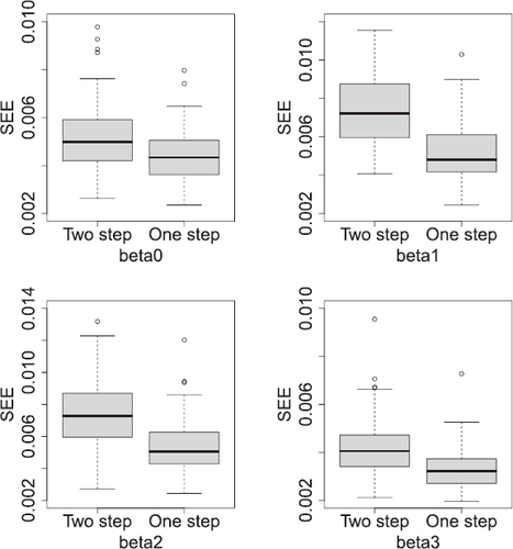We repeat the simulation 100 times with time series length $T=400$, and thus have 100 values of SEE defined in (5.2) for each of ${\beta }_j(\cdot )$, $j=0,1,2,3$, with the one-step and the two-step methods, respectively, summarized in boxplots in Figure 1 with the four panels for ${\beta }_0(\cdot )$, ${\beta }_1(\cdot )$, ${\beta }_2(\cdot )$, and ${\beta }_3(\cdot )$, respectively. The results clearly show that the one-step method has consistently smaller SEE values than the two-step method, and hence gets more accurate estimation than the two-step method for the considered T and N.

Figure 1: Boxplots of 100 Monte Carlo SEE values defined in (5.2) for the estimation of ${\beta }_j(\cdot ,\cdot )$, $j=0,1,2,3$, in the four panels, where the two-step (left) and the one-step (right) with $T=400$ and $N=23$ are presented in each panel.

Second, we compare the performances of the one-step method under three different time series sample sizes of $T=200$, $T=400$, and $T=600$, respectively. We repeat the Monte Carlo simulation 100 times, and thus obtain 100 SEE values defined in (5.2) for each of ${\beta }_j(\cdot )$, $j=0,1,2,3$, with the DyFAST (5.1) by the one-step estimation method, summarized in boxplots in Figure A.1 in Appendix A.5. As expected, from Figure A.1, with the time series sample size increasing, the accuracy of the estimation of the ${\beta }_j(\cdot )$’s apparently improves. As shown, our Scheme 1 given in Section 3 can work well even for the sample size $T=200$.

Third, we examine Scheme 2 with the fusing/combining procedure of spatial weight matrices in Section 4 by estimating the combining weight a. Here we suppose the true spatial weight matrix $W=0.6W_1+0.4W_2$ with $a_1=a=0.6$ and $a_2=1-a=0.4$ as given in (4.1), in model (5.1). We consider the estimation with Scheme 2 under three time series sample sizes of $T=200$, $T=400$, and $T=600$, respectively. Figure A.2 in Appendix A.5 shows the boxplots of 100 Monte Carlo values for the estimation of a, under $T=200$, $T=400$ and $T=600$, respectively, which appears rather acceptable with the median of the 100 estimates of a very close to 0.6 even for the sample size $T=200$.

Figure 2: Boxplots of 100 Monte Carlo SEE values for the estimation of ${\beta }_j(\cdot )$, $j=0,1,2,3$, with $T=400$ and $N=23$, for the DyFAST under the real (oracle) spatial weight matrix ($W=0.6W_1+0.4W_2$) and the estimated combined spatial weight matrix ($\widehat{W}={\widehat{a}}_1{W}_1+{\widehat{a}}_2{W}_2$), respectively, in each panel.

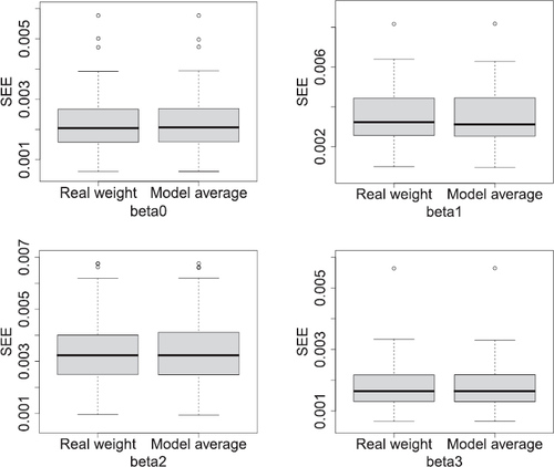
We further examine the impacts of the estimated combined weight matrix on the estimation of the coefficient functions of the DyFAST model. Figure 2 displays boxplots of the 100 Monte Carlo SEE values defined in (5.2) for the estimation of ${\beta }_j(\cdot )$, $j=0,1,2,3$, under the real spatial weight matrix W and the estimated combined spatial weight matrix $\widehat{W}=\widehat{a}{W}_1+(1-\widehat{a})W_2$, respectively, under the sample size $T=400$. Moreover, Figure A.3 in Appendix A.5 presents the mean of the 100 Monte Carlo estimates of ${\beta }_j(\cdot )$, $j=0,1,2,3$ with the DyFAST under the true spatial weight matrix W (in dotted lines) and the estimated combined spatial weight matrix $\widehat{W}$ (in dashed lines), respectively, when compared with the true curves plotted in solid lines. We observe from both Figures 2 and A.3 that our estimates ${\beta }_j(\cdot )$, $j=0,1,2,3$ mimic the corresponding true curves quite well even for the relatively small size $T=200$. The estimation results indicate that with our estimated combined spatial weight matrix, our DyFAST method can still accurately estimate the coefficient functions.

Moreover, we examine the efficiency of the estimation in the case that the true combined spatial weight matrix contains negative combining weight in the form $W=1.2W_1-0.2W_2$ with $a_1=a=1.2$ and $a_2=1-a=-0.2$. Figure A.4 in Appendix A.5 shows the boxplots of the 100 Monte Carlo values for estimation of $a_1=a$ and $a_2=1-a$ under $T=400$. It clearly follows from Figure A.4 that the proposed procedure can also accurately identify the negative combining weight for the candidate spatial weight matrices. The impacts of the estimated weight matrix on the estimation of the coefficient functions are omitted with similar outcomes as reported above. To sum up, these findings further demonstrate that our DyFAST method works very well with Scheme 2 even for the combined spatial weight matrix with negative combining weights.

6 Real Data Example

6.1 Background and Data

Retail gasoline prices are considerably fluctuating over time and across countries within the Europe. Numerous studies have examined the impact of crude oil price on retail gasoline prices, particularly focusing on the asymmetries in price transmission (see Wlazlowski et al. 2009; Clerides 2010). Any price dis-equilibria of retail gasoline in neighbor countries can cause “fuel travels” and create significantly cross-national spatial price spillovers in EU countries (Banfi, Filippini, and Hunt 2005; Wlazlowski et al. 2009). Negligence of the spatial dependency may hence cause a biased result. To better measure the price transmission of the retail gasoline in the EU, we will apply our DyFAST analysis in this study.

Our data consist of panel data of weekly spot prices for Brent crude oil price and diesel prices in $N=23$ European countries from January 26, 2015 to December 19, 2016. The data are obtained from European Commission (Source from: https://ec.europa.eu/energy/en/data-analysis/weekly-oil-bulletin), with all commodity prices expressed in EUR and the diesel prices inclusive of duties and taxes (Wlazlowski et al. 2009). The descriptive statistics for the raw data are reported in Table A.1 in Appendix A.5. As all the series at the price level are nonstationary (see, Table A.1), we will consider the data at the return level by computing the Brent crude oil price return ($X_t$) and the diesel prices return ($Y_{it}=Y_t(s_i)$), through the difference in the logarithm of two consecutive weekly prices, multiplied by 100. For such country-level data, as usual, we take $s_i=(u_i,v_i)$ to be the centroid (latitude and longitude, scaled down by 100) for country i, $i=1,2,\dots ,N(=23)$, in the EU, where we have got the latitude and longitude scaled down by 100 for easy operations of nonparametric smoothing; see Figure A.5 in Appendix A.5 for the locations plotted. In the analysis as a demonstration, we took a simple and easy way to see, by a view of infill asymptotic, the centroid locations $s_i$’s simply as the observing locations in a continuous domain $S(\subset R^2)$ of the EU, and the data as a realization of a space-continuous process indexed by location $s\in S$ in space, not of a “constant-by-area” process or a spatially discrete process, in population. See more discussions on this in Appendix A.6.

Table 1: Country groups.

Group 1	Belgium Germany Denmark Luxembourg Netherlands Portugal Sweden
Group 2	Austria Czech.Republic Estonia Spain Finland France Italy Lithuania
	Latvia Poland Slovenia Slovakia
Group 3	Bulgaria Greece Hungary Romania

NOTE: The groups are classified based on Figure A.8 in Appendix A.4.

6.2 The DyFAST Analysis

We are modeling the diesel prices return $Y_{it}=Y_t(s_i)$ for country $s_i$ by our DyFAST model (2.2) associated with the Brent crude oil price return ($X_t$), that is $X_t(s_i)=:X_t$ for different countries. In estimating the spatial neighboring effect for diesel prices, there are different candidate weight matrices. In this study, for example, we can consider two pre-specified spatial weight matrices $W_1$ and $W_2$, which are distance based. Let the centroid distances from each spatial unit (country) i to all other units $j\ne i$ be ranked as follows: $d_{i{j}_i(1)}\le d_{i{j}_i(2)}\le \cdots \le d_{i{j}_i(N-1)}$, where $N=23$, and $d_{ij}$ is the Euclidean distance between the centroids of two countries $s_i$ and $s_j$, and $j_i(k)$ stands for the country that is the kth closest to country i. Then for each $k=1,\dots ,N-1$, the set ${\mathcal{N}}_k(i)=\{j_i(1),j_i(2),\dots ,j_i(k)\}$ contains the k closest units to unit i. Then for $W_1,$ we consider $k=2$, and ${\mathcal{N}}_2(i)=\{j_i(1),j_i(2)\}$ containing the 2 closest units to unit i. The elements of $W_1$ are set as $w_{ij}=1/d_{ij}$ for $j\in {\mathcal{N}}_2(i)$, and $w_{ij}=0$ otherwise. For $W_2$, we consider all neighboring countries with $w_{ij}=1/d_{ij}$, for $j\in {\mathcal{N}}_{22}(i)$ with $k=22$. All spatial weight matrices are then row-wise standardized, which we still denote as $W_1$ and $W_2$ below.

First, we apply the DyFAST to estimate the spatial neighboring effect for diesel price returns by Scheme 1, with $W_1$ and $W_2$ considered as follows:(6.1) $$\begin{array}{cc}{Y}_t(s_i)={\beta }_0(X_t(s_i),s_i)+{\sum }_{j=1}^p{\beta }_j^{(1)}(X_t(s_i),s_i)Y_{t-j}^{\text{SL}(1)}(s_i)\hfill & \hfill \\ \hspace{1em}+{\sum }_{j=1}^p{\beta }_j^{(2)}(X_t(s_i),s_i)Y_{t-j}^{\text{SL}(2)}(s_i)\hfill & \hfill \\ \hspace{1em}+{\sum }_{l=1}^q{\beta }_{p+l}(X_t(s_i),s_i)Y_{t-l}(s_i)+{\epsilon }_t(s_i),\hfill & \hfill \end{array}$$(6.1) where $Y_{t-j}^{\text{SL}(1)}(s_i)$ and $Y_{t-j}^{\text{SL}(2)}(s_i)$ are defined as in (2.1) with $W_1$ and $W_2$, respectively, and the functional autoregressive coefficients are as given in (4.4). Because the $s_i$’s are irregularly positioned in space, we simply see them as the observing locations in space that is continuous as in geostatistics (see, Cressie 1993), in particular, in view of that fact that citizens of EU member countries can move freely around the countries of the EU. We therefore put the functional coefficients $\beta (x,s)$’s in (6.1) as smooth functions of $(x,s)$ as done in Lu et al. (2009) and Al-Sulami et al. (2017). The orders $(p,q)$ of spatial neighboring and temporal lagged autoregressive effects are determined by Akaike Information Criterion with correction (AICc), which are listed in Table A.2 in Appendix A.5, with the model of optimal orders $p=2$ and $q=1$ as follows(6.2) $$\begin{array}{cc}{Y}_t(s_i)={\beta }_0(X_t(s_i),s_i)+{\sum }_{j=1}^2{\beta }_j^{(1)}(X_t(s_i),s_i)Y_{t-j}^{\text{SL}(1)}(s_i)\hfill & \hfill \\ \hspace{1em}+{\sum }_{j=1}^2{\beta }_j^{(2)}(X_t(s_i),s_i)Y_{t-j}^{\text{SL}(2)}(s_i)\hfill & \hfill \\ \hspace{1em}+{\beta }_3(X_t(s_i),s_i)Y_{t-l}(s_i)+{\epsilon }_t(s_i).\hfill & \hfill \end{array}$$(6.2)

Table 2: Comparison of forecasting results.

Model (6.2)	Model (6.3)	Model (6.4)	Threshold	LinearSpat	LinearAR
1.635	1.570	1.557	1.507	1.875	2.212

NOTE: This table shows the Mean Squared Prediction Error (MSPE) of the one-step ahead prediction evaluated by the last $T_f=15$ observations for DyFAST with $(W_1,W_2)$ (Model (6.2)), DyFAST with combined spatial weight matrix (Model (6.3)), DyFAST with $W_2$ (Model (6.4)), DyFAST with nonlinear threshold functions (Threshold) and linear model with spatial lags (LinearSpat) and linear AR without spatial lags (LinearAR).

Moreover, the bandwidths used for estimation are decided by cross-validation, which are $h_1=3.187$ and $h_2=0.275$, respectively. Figure A.6 in Appendix A.5 shows the estimated coefficient functions of model (6.2). We can see that the functions ${\beta }_1^{(1)}(x,s_i)$ depicted in the top-middle panel and ${\beta }_2^{(1)}(x,s_i)$ in the top-right panel in Figure A.6, both of which are as functions of x with $i=1,\dots ,N$, associated with $W_1$, appear to fluctuate around zero mostly. Intuitively, with more neighboring countries considered in $W_2$, it would be more important as indicated in bottom left and middle panels of Figure A.6. Therefore, we are considering the DyFAST by combining spatial weight matrices $W_1$ and $W_2$ to see whether the combining weight $a_1$ is statistically significant by Scheme 2:(6.3) $$\begin{array}{cc}{Y}_t(s_i)={\beta }_0(X_t(s_i),s_i)+{\sum }_{j=1}^2{\beta }_j(X_t(s_i),s_i)\left({\sum }_{k=1}^2{a}_k{Y}_{t-j}^{\text{SL}(\mathrm{k})}(s_i)\right)\hfill & \hfill \\ +{\beta }_3(X_t(s_i),s_i)Y_{t-l}(s_i)+{\epsilon }_t(s_i),\hfill & \hfill \end{array}$$(6.3) where $a_1$ and $a_2$ are two constants, satisfying $a_1+a_2=1$. Moreover, the used bandwidths are decided by cross-validation, which are $h_1=3.201$ and $h_2=0.273$, respectively. Then we can obtain the estimated combining weight vector ($a_1=-0.23$, $a_2=1.23$), and the estimated functional coefficients ${\beta }_j(x,s_i)$, $j=0,1,2$, are plotted in Figure A.7 in Appendix A.5. To test whether the $a_k$ is statistically significant, we consider a bootstrap approach as the asymptotic variance of the estimator appears complex (see, Theorem 4.2). Given the observed sample $\{(X_t(s_i),Y_t(s_i))$, $t=1,\dots ,T$, $i=1,\dots ,N\}$, the method proceeds as detailed in the Algorithm (Bootstrap for DyFAST) given in Appendix A.7.

By repeating the bootstrap 1000 times, we can obtain the t-values for $a_1$ and $a_2$ based on the replications, which are equal to $-0.4956$ and 2.7506, with the corresponding p-values equal to 0.6203 and 0.0061, respectively. These show that $a_1$ is not, while $a_2$ is, statistically significant at 1% significance level, which indicates that our method selects $W_2$ as the optimal weight matrix ($a_1=0$ and $a_2=1$). The top middle and right sub-figures in Figure A.7 further confirm that $a_1{\beta }_1(x,s_i)$ and $a_1{\beta }_2(x,s_i)$ as functions of x fluctuate nearly close to zero.

We now consider only $W_2$ to investigate the impacts of Brent crude oil price return on diesel price returns in the $N=23$ EU countries, which is of a form(6.4) $$\begin{array}{cc}{Y}_t(s_i)={\beta }_0(X_t,s_i)+{\sum }_{j=1}^2{\beta }_j(X_t,s_i)Y_{t-j}^{\text{SL}(2)}(s_i)\hfill & \hfill \\ \hspace{1em}+{\beta }_3(X_t,s_i)Y_{t-1}(s_i)+{\epsilon }_t(s_i).\hfill & \hfill \end{array}$$(6.4)

Figure A.8 in Appendix A.5 shows the estimated ${\beta }_j(x,s_i)$’s as a function of x for the ith country, with the bandwidths $h_1=3.293$ and $h_2=0.274$. Here we can see that for temporal lag equal to 1, the spatial neighboring effects (i.e., ${\beta }_1(x,s_i)$) are positive. Further, from Figure A.7, ${\beta }_2(x,s_i)$ (especially at the right side) and ${\beta }_3(x,s_i)$ (especially at the left side), as functions of x, can be categorized as three groups, as given in Table 1, with higher, medial or lower valued coefficients, respectively, for different $s_i$’s (i.e., the centroids, as representing locations, of different countries) . Such a division is useful for parameterization of the thresholds used for forecasting in Appendix A.8. Note that, for simplicity, we put $s_i$’s as usual the centroids, representing locations, of different countries, which are actually separated though both countries among them may be neighbored. Here the Group 1 countries are basically located in North-Western Europe (except Portugal), and the Group 3 countries are located in Balkans, while the other countries belonging to Group 2 are in the middle belt between them. Finally, from Figure A.8, the self temporal lag effects (i.e., ${\beta }_3(x,s_i)$) are positive and relatively larger for Group 3 than those for Group 1 (near zero) and Group 2 (negative). These empirical findings seem to be interesting, which may help governments and energy users to mitigate the negative impacts from the expected or unexpected fluctuations in the oil and the neighboring retail gasoline markets and to better manage energy risk. Moreover, the local country governments may formulate relevant energy policies on the basis of their geographical locations.

To further evaluate our methods and findings in application, we have compared the one-step ahead prediction performances of our DyFAST specifications (6.2)–(6.4) together with threshold parameterization of the smoothing coefficients in (6.4) (denoted by ‘Threshold’; see, Appendix A.8) as well as the (location-wise) linear model with spatial lags (i.e., (6.4) with the ${\beta }_j$ coefficients independent of x; denoted by “LinearSpat”) and the (location-wise) time series linear AR model (i.e., the mentioned LinearSpat model without considering spatial lag terms; denoted by LinearAR). The corresponding Mean Squared Prediction Errors (MSPEs) for one-step ahead forecasting are reported in Table 2 with the details presented in Appendix A.9, where we set aside the last $T_f=15$ data for forecasting evaluation and used the first $T=76$ data as training set. Clearly, our DyFAST model and schemes can well uncover the nonlinear effects of the crude oil price fluctuations on the retail gasoline prices with prediction significantly improved by our models, especially the “Threshold” model with the smallest MSPE of 1.507, as indicated in Table 2; see Appendix A.8 for more discussions.

In summary, our proposed methodologies can help to meet the challenges well in our setting, especially: (a) the irregularly positioned locations that make it hard to characterize the neighboring effects for selection of an optimal spatial weight matrix for forecasting; (b) the spatio-temporal dependencies with location-wide non-stationarity making it difficult to characterize the mutual interactions for a dynamic system across time and space; (c) the complex spatio-temporal interactions that make it hard to build an efficient procedure for computation of the estimation. We have hence proposed two DyFAST models characterizing nonlinear dynamic behavior of regime-switching nature, with two different estimation schemes defining spatial weight matrices together with one- and two-step procedures for estimation developed. The asymptotic theories for these estimation schemes are then established. Both simulation and real data examples have demonstrated the usefulness of the proposed methods in nonlinear analysis of spatio-temporal data.

Acknowledgments

The authors are grateful to the Editor, Associate Editor, and two referees for their helpful comments for improvement of this article. All the authors contributed equally with names listed in an alphabetical order.

Key Projects of National Natural Science Foundation of Zhejiang Province;National Natural Science Foundation of China;Natural Science Foundation of Hunan Province;

Supplementary Materials

In the “Appendix: supplementary materials” file, we have collected the related supplementary materials with regularity conditions in Appendix A.1, practical bandwidth and model order selection in Appendix A.2, proofs for Sections 3 and 4 in Appendix A.3 and Appendix A.4, respectively, additional figures and tables for Sections 5 and 6 in Appendix A.5, more discussions on viewing data, locations and space continuous process in population for Section 6 in Appendix A.6, the bootstrap procedure for Section 6 in Appendix A.7, and evaluation of prediction for Section 6 in Appendix A.8.

Additional information

Funding

This research was partially supported by the EU’s Marie Curie career integration grant PCIG14-GA-2013-631692, British Academy/Leverhulme Trust (No.SG162909), NSFC (No. 71971131, 12171427, U21A20426), NSF of Hunan Province (2022JJ40647), Zhejiang Provincial NSF (No. LZ21A010002) and the Fundamental Research Funds for the Central Universities (2021XZZX002), which are acknowledged.

References

- Al-Sulami, D., Jiang, Z., Lu, Z., and Zhu, J. (2017), “Estimation for Semiparametric Nonlinear Regression of Irregularly Located Spatial Time-Series Data,” Econometrics and Stats, 2, 22–35. DOI: 10.1016/j.ecosta.2017.01.002.
- Anselin, L. (1988), Spatial Econometrics: Methods and Models, Dordrecht: Springer.
- Banfi, S., Filippini, M., and Hunt, L. C. (2005), “Fuel Tourism in Border Regions: The Case of Switzerland,” Energy Economics, 27, 689–707. DOI: 10.1016/j.eneco.2005.04.006.
- Box, G. E., Jenkins, G. M., Reinsel, G. C., and Ljung, G. M. (2015), Time Series Analysis: Forecasting and Control, Hoboken, NJ: Wiley.
- Cai, Z., Fan, J., and Yao, Q. (2000), “Functional-Coefficient Regression Models for Nonlinear Time Series,” Journal of the American Statistical Association, 95, 941–956. DOI: 10.1080/01621459.2000.10474284.
- Chen, R., and Tsay, R. S. (1993), “Functional-Coefficient Autoregressive Models,” Journal of the American Statistical Association, 88, 298–308. DOI: 10.2307/2290725.
- Clerides, S., (2010), “Retail Fuel Price Response to Oil Price Shocks in EU Countries,” Cyprus Economic Policy Review, 4, 25–45.
- Cliff, A., and Ord, K. (1972), “Testing for Spatial Autocorrelation among Regression Residuals,” Geographical Analysis, 4, 267–284. DOI: 10.1111/j.1538-4632.1972.tb00475.x.
- Comber, A., and Wulder, M. (2019), “Considering Spatiotemporal Processes in Big Data Analysis: Insights from Remote Sensing of Land Cover and Land Use,” Transactions in GIS, 23, 879–891. DOI: 10.1111/tgis.12559.
- Cressie, N., (1993), Statistics For Spatial Data, New York: Wiley.
- Cressie, N., and Wikle, C. K. (2015), Statistics for Spatio-Temporal Data, Hoboken, NJ: Wiley.
- Fan, J., and Gijbels, I. (1996), Local Polynomial Modelling and Its Applications. Monographs on Statistics and Applied Probability 66. Boca Ratoon, FL: CRC Press.
- Fan, J., and Yao, Q. (2003), Nonlinear Time Series: Nonparametric and Parametric Methods, New York: Springer.
- Fan, J., and Zhang, W. (1999), “Statistical Estimation in Varying Coefficient Models,” The Annals of Statistics, 27, 1491–1518. DOI: 10.1214/aos/1017939139.
- Gao, J. (2007), Nonlinear Time Series: Semiparametric and Nonparametric Methods, Boca Raton, FL: CRC Press.
- Gao, J., Lu, Z., and Tjøstheim, D. (2006), “Estimation in Semiparametric Spatial Regression,” The Annals of Statistics, 34, 1395–1435. DOI: 10.1214/009053606000000317.
- Gelfand, A. E., Kim, H. J., Sirmans, C., and Banerjee, S. (2003), “Spatial Modeling with Spatially Varying Coefficient Processes,” Journal of the American Statistical Association, 98, 387–396. DOI: 10.1198/016214503000170.
- Hallin, M., Lu, Z., and Tran, L. T. (2004), “Local Linear Spatial Regression,” The Annals of Statistics, 32, 2469–2500. DOI: 10.1214/009053604000000850.
- LeSage, J., and Pace, R. K. (2009), Introduction to Spatial Econometrics, Boca Raton, FL: CRC Press.
- Lu, Z., Steinskog, D. J., Tjøstheim, D., and Yao, Q. (2009), “Adaptively Varying-Coefficient Spatiotemporal Models,” Journal of the Royal Statistical Society, Series B, 71, 859–880. DOI: 10.1111/j.1467-9868.2009.00710.x.
- Lu, Z., Tjøstheim, D., and Yao, Q. (2008), “Smoothing, Nugget Effect and Infill Asymptotics,” Statistics and Probability Letters, 78, 3145–3151. DOI: 10.1016/j.spl.2008.06.002.
- Ord, K., (1975), “Estimation Methods for Models of Spatial Interaction,” Journal of the American Statistical Association, 70, 120–126. DOI: 10.1080/01621459.1975.10480272.
- Subba Rao, S., (2008), “Statistical Analysis of a Spatio-Temporal Model with Location-Dependent Parameters and a Test for Spatial Stationarity,” Journal of Time Series Analysis, 29, 673–694. DOI: 10.1111/j.1467-9892.2008.00577.x.
- Sun, Y., Yan, H., Zhang, W., and Lu, Z. (2014), “A Semiparametric Spatial Dynamic Model,” Annals of Statistics, 42, 700–727.
- Teräsvirta, T., Tjøstheim, D., and Granger, C. (2010), Modelling Nonlinear Economic Time Series, Oxford: Oxford University Press.
- Tong, H., (1990), Non-linear Time Series: A Dynamical System Approach, Oxford: Oxford University Press.
- Wlazlowski, S., Giulietti, M., Binner, J., and Milas, C. (2009), “Price Dynamics in European Petroleum Markets,” Energy Economics, 31, 99–108. DOI: 10.1016/j.eneco.2008.08.009.
- Zhang, X., and Yu, J. (2018), “Spatial Weights Matrix Selection and Model Averaging for Spatial Autoregressive Models,” Journal of Econometrics, 203, 1–18. DOI: 10.1016/j.jeconom.2017.05.021.