Adaptive Functional Thresholding for Sparse Covariance Function Estimation in High Dimensions

Abstract

Covariance function estimation is a fundamental task in multivariate functional data analysis and arises in many applications. In this article, we consider estimating sparse covariance functions for high-dimensional functional data, where the number of random functions p is comparable to, or even larger than the sample size n. Aided by the Hilbert–Schmidt norm of functions, we introduce a new class of functional thresholding operators that combine functional versions of thresholding and shrinkage, and propose the adaptive functional thresholding estimator by incorporating the variance effects of individual entries of the sample covariance function into functional thresholding. To handle the practical scenario where curves are partially observed with errors, we also develop a nonparametric smoothing approach to obtain the smoothed adaptive functional thresholding estimator and its binned implementation to accelerate the computation. We investigate the theoretical properties of our proposals when p grows exponentially with n under both fully and partially observed functional scenarios. Finally, we demonstrate that the proposed adaptive functional thresholding estimators significantly outperform the competitors through extensive simulations and the functional connectivity analysis of two neuroimaging datasets. Supplementary materials for this article are available online.

KEYWORDS:

• Binning
• Functional connectivity
• Functional sparsity
• High-dimensional functional data
• Local linear smoothing
• Partially observed functional data

1 Introduction

The covariance function estimation plays an important role in functional data analysis, while existing methods are restricted to data with a single or small number of random functions. Recent advances in technology have made multivariate or even high-dimensional functional datasets increasingly common in various applications: for example, time-course gene expression data in genomics (Storey et al. 2005), air pollution data in environmental studies (Kong et al. 2016) and different types of brain imaging data in neuroscience (Li and Solea 2018; Qiao, Guo, and James 2019). Under such scenarios, suppose we observe n independent samples ${\mathbf{X}}_i(·)={\{X_{i1}(·),\dots ,X_{ip}(·)\}}^{\mathrm{T}}$ for $i=1,\dots ,n$ defined on a compact interval $\mathcal{U}$ with covariance function $$\mathbf{\Sigma }(u,v)={\{{\Sigma }_{jk}(u,v)\}}_{p\times p}=\text{cov}\{{\mathbf{X}}_i(u),{\mathbf{X}}_i(v)\}, u,v\in \mathcal{U}.$$

From a heuristic interpretation, we can simply treat each curve $X_{ij}(·)$ as an infinitely long vector and replace the (j, k)th entry of $\mathbf{\Sigma }$ by ${\Sigma }_{jk}(·,·)=\text{cov}\{X_{ij}(·),X_{ik}(·)\},$ the cross-covariance matrix of two infinitely long vectors. Then $\mathbf{\Sigma }$ can be understood as a block matrix with infinite sizes and its (j, k)th block being ${\Sigma }_{jk}(·,·).$ Besides being of interest in itself, an estimator of $\mathbf{\Sigma }$ is useful for many applications including, for example, multivariate functional principal components analysis (FPCA) (Happ and Greven 2018), multivariate functional linear regression (Chiou, Yang, and Chen 2016), functional factor model (Guo, Qiao, and Wang 2022) and functional classification (Park, Ahn, and Jeon 2021). See Section 2.3 for details.

Our article focuses on estimating $\mathbf{\Sigma }$ under high-dimensional scaling, where p can be comparable to, or even larger than n. In this setting, the sample covariance function $$\begin{array}{c}\widehat{\mathbf{\Sigma }}(u,v)={\{{\widehat{\Sigma }}_{jk}(u,v)\}}_{p\times p}\\ =\frac{1}{n-1}\sum _{i=1}^n\{{\mathbf{X}}_i(u)-\overline{\mathbf{X}}(u)\}{\{{\mathbf{X}}_i(v)-\overline{\mathbf{X}}(v)\}}^{\mathrm{T}}, u,v\in \mathcal{U},\end{array}$$where $\overline{\mathbf{X}}(·)=n^{-1}{\sum }_{i=1}^n{\mathbf{X}}_i(·),$ performs poorly, and some lower-dimensional structural assumptions need to be imposed to estimate $\mathbf{\Sigma }$ consistently. In contrast to extensive work on estimating high-dimensional sparse covariance matrices (Bickel and Levina 2008; Rothman, Levina, and Zhu 2009; Cai and Liu 2011; Chen and Leng 2016; Avella-Medina et al. 2018; Wang et al. 2021), research on sparse covariance function estimation in high dimensions remains largely unaddressed in the literature.

In this article, we consider estimating sparse covariance functions via adaptive functional thresholding in the sense of shrinking some blocks ${\widehat{\Sigma }}_{jk}(·,·)$’s in an adaptive way. To achieve this, we introduce a new class of functional thresholding operators that combine functional versions of thresholding and shrinkage based on the Hilbert-Schmidt norm of functions, and develop an adaptive functional thresholding procedure on $\widehat{\mathbf{\Sigma }}(·,·)$ using entry-dependent functional thresholds that automatically adapt to the variability of blocks ${\widehat{\Sigma }}_{jk}(·,·)$’s. To provide theoretical guarantees of our method under high-dimensional scaling, it is essential to develop standardized concentration results taking into account the variability adjustment. Compared with adaptive thresholding for nonfunctional data (Cai and Liu 2011), the intrinsic infinite-dimensionality of each $X_{ij}(·)$ leads to a substantial rise in the complexity of sparsity modeling and theoretical analysis, as one needs to rely on some functional norm of standardized ${\widehat{\Sigma }}_{jk}$’s, for example, the Hilbert–Schmidt norm, to enforce the functional sparsity in $\widehat{\mathbf{\Sigma }}$ and tackle more technical challenges for standardized processes within an abstract Hilbert space. To handle the practical scenario where functions are partially observed with errors, it is desirable to apply nonparametric smoothers in conjunction with adaptive functional thresholding. This poses a computationally intensive task especially when p is large, thus calling for the development of fast implementation strategy.

There are many applications of the proposed sparse covariance function estimation method in neuroimaging analysis, where brain signals are measured over time at a large number of regions of interest (ROIs) for individuals. Examples include the brain-computer interface classification (Lotte et al. 2018) and the brain functional connectivity identification (Rogers et al. 2007). Traditional neuroimaging analysis models brain signals for each subject as multivariate random variables, where each ROI is represented by a random variable, and hence the covariance/correlation matrices of interest are estimated by treating the time-course data of each ROI as repeated observations. However, due to the nonstationary and dynamic features of signals (Chang and Glover 2010), the strategy of averaging over time fails to characterize the time-varying structure leading to the loss of information in the original space. To overcome these drawbacks, we follow recent proposals to model signals directly as multivariate random functions with each ROI represented by a random function (Li and Solea 2018; Qiao, Guo, and James 2019; Zapata, Oh, and Petersen 2022; Lee et al. in press). The identified functional sparsity pattern in our estimate of $\mathbf{\Sigma }$ can be used to recover the functional connectivity network among different ROIs, which is illustrated using examples of functional magnetic resonance imaging (fMRI) datasets in Section 6 and Section E.3 of the supplementary material.

Our article makes useful contributions at multiple fronts. On the method side, it generalizes the thresholding/sparsity concept in multivariate statistics to the functional setting and offers a novel adaptive functional thresholding proposal to handle the heteroscedastic problem of the sparse covariance function estimation motivated from neuroimaging analysis and many statistical applications, for example, those in Section 2.3 and Section C.2 of the supplementary material. It also provides an alternative way of identifying correlation-based functional connectivity with no need to specify the correlation function, the estimation of which poses challenges as the inverses of ${\Sigma }_{jj}(u,v)$’s are unbounded. In practice when functions are observed with errors at either a dense grid of points or a small subset of points, we also develop a unified local linear smoothing approach to obtain the smoothed adaptive functional thresholding estimator and its fast implementation via binning (Fan and Marron 1994) to speed up the computation without sacrificing the estimation accuracy. On the theory side, we show that the proposed estimators enjoy the convergence and support recovery properties under both fully and partially observed functional scenarios when p grows exponentially fast relative to n. The proof relies on tools from empirical process theory due to the infinite-dimensional nature of functional data and some novel standardized concentration bounds in the Hilbert–Schmidt norm to deal with issues of high-dimensionality and variance adjustment. Our theoretical results and adopted techniques are general, and can be applied to other settings in high-dimensional functional data analysis.

The remainder of this article is organized as follows. Section 2 introduces a class of functional thresholding operators, based on which we propose the adaptive functional thresholding of the sample covariance function. We then discuss a couple of applications of the sparse covariance function estimation. Section 3 presents convergence and support recovery analysis of our proposed estimator. In Section 4, we develop a nonparametric smoothing approach and its binned implementation to deal with partially observed functional data, and then investigate its theoretical properties. In Sections 5 and 6, we demonstrate the uniform superiority of the adaptive functional thresholding estimators over the universal counterparts through an extensive set of simulation studies and the functional connectivity analysis of a neuroimaging dataset, respectively. All technical proofs are relegated to the supplementary material. We also provide the codes to reproduce the results for simulations and real data analysis in supplementary materials.

2 Methodology

2.1 Functional Thresholding

We begin by introducing some notation. Let $L_2(\mathcal{U})$ denotes a Hilbert space of square integrable functions defined on $\mathcal{U}$ and $\mathbb{S}=L_2(\mathcal{U})\otimes L_2(\mathcal{U}),$ where ⊗ is the Kronecker product. For any $Q\in \mathbb{S},$ we denote its Hilbert–Schmidt norm by $\left|\right|Q|{|}_{\mathcal{S}}={\left\{\int \int Q{(u,v)}^2\text{dudv}\right\}}^{1/2}.$ With the aid of Hilbert–Schmidt norm, for any regularization parameter $\lambda \ge 0,$ we first define a class of functional thresholding operators $s_{\lambda }: \mathbb{S}\to \mathbb{S}$ that satisfy the following conditions:

1. $\left|\right|s_{\lambda }(Z)|{|}_{\mathcal{S}}\le c|\left|Y\right|{|}_{\mathcal{S}}$ for all Z and $Y\in \mathbb{S}$ that satisfy $\left|\right|Z-Y|{|}_{\mathcal{S}}\le \lambda$ and some $c>0;$

2. $\left|\right|s_{\lambda }(Z)|{|}_{\mathcal{S}}=0$ for $\left|\right|Z|{|}_{\mathcal{S}}\le \lambda ;$

3. $\left|\right|s_{\lambda }(Z)-Z|{|}_{\mathcal{S}}\le \lambda$ for all $Z\in \mathbb{S}.$

Our proposed functional thresholding operators can be viewed as the functional generalization of thresholding operators (Cai and Liu 2011). Instead of a simple pointwise extension of such thresholding operators under functional domain, we advocate a global thresholding rule based on the Hilbert–Schmidt norm of functions that encourages the functional sparsity, in the sense that $s_{\lambda }(Z)(u,v)=0$, for all $u,v\in \mathcal{U},$ if $\left|\right|Z|{|}_{\mathcal{S}}\le \lambda$ under condition (ii). Condition (iii) limits the amount of (global) functional shrinkage in the Hilbert–Schmidt norm to be no more than $\lambda .$

Conditions (i)–(iii) are satisfied by functional versions of some commonly adopted thresholding rules, which are introduced as solutions to the following penalized quadratic loss problem with various penalties: (1) $$s_{\lambda }(Z)=\underset{\theta \in \mathbb{S}}{\arg \min }\left\{\frac{1}{2}\left|\right|\theta -Z|{|}_{\mathcal{S}}^2+p_{\lambda }(\theta )\right\}$$(1) with $p_{\lambda }(\theta )={\tilde{p}}_{\lambda }(|\left|\theta \right|{|}_{\mathcal{S}})$ being a penalty function of $\left|\right|\theta |{|}_{\mathcal{S}}$ to enforce the functional sparsity.

The soft functional thresholding rule results from solving (1) with an ${\mathcal{l}}_1/{\mathcal{l}}_2$ type of penalty, $p_{\lambda }(\theta )=\lambda \left|\right|\theta |{|}_{\mathcal{S}},$ and takes the form of $s_{\lambda }^{\mathrm{S}}(Z)=Z{(1-\lambda /|\left|Z\right|{|}_{\mathcal{S}})}_{+},$ where ${(x)}_{+}=\max (x,0)$ for $x\in \mathbb{R}.$ This rule can be viewed as a functional generalization of the group lasso solution under the multivariate setting (Yuan and Lin 2006). To solve (1) with an ${\mathcal{l}}_0/{\mathcal{l}}_2$ type of penalty, $p_{\lambda }(\theta )=2^{-1}{\lambda }^{2}I(|\left|\theta \right|{|}_{\mathcal{S}}\ne 0),$ we obtain hard functional threhsolding rule as $ZI(|\left|Z\right|{|}_{\mathcal{S}}\ge \lambda ),$ where $I(·)$ is an indicator function. As a comparison, soft functional thresholding corresponds to the maximum amount of functional shrinkage allowed by condition (iii), whereas no shrinkage results from hard functional thresholding. Taking the compromise between soft and hard functional thresholding, we next propose functional versions of SCAD (Fan and Li 2001) and adaptive lasso (Zou 2006) thresholding rules. With a SCAD penalty (Fan and Li 2001) operating on $\left|\right|·|{|}_{\mathcal{S}}$ instead of $|·|$ for the univariate scalar case, SCAD functional thresholding $s_{\lambda }^{\text{SC}}(Z)$ is the same as soft functional thresholding if $\left|\right|Z|{|}_{\mathcal{S}}<2\lambda ,$ and equals $Z\{(a-1)-a\lambda /|\left|Z\right|{|}_{\mathcal{S}}\}/(a-2)$ for $\left|\right|Z|{|}_{\mathcal{S}}\in [2\lambda ,a\lambda ]$ and Z if $\left|\right|Z|{|}_{\mathcal{S}}>a\lambda ,$ where $a>2.$ Analogously, adaptive lasso functional thresholding rule is $s_{\lambda }^{\text{AL}}(Z)=Z{(1-{\lambda }^{\eta +1}/|\left|Z\right|{|}_{\mathcal{S}}^{\eta +1})}_{+}$ with $\eta \ge 0.$

Our proposed functional generalizations of soft, SCAD and adaptive lasso thresholding rules can be checked to satisfy conditions (i)–(iii), see Section B.1 of the supplementary material for details. To present a unified theoretical analysis, we focus on functional thresholding operators $s_{\lambda }(Z)$ satisfying conditions (i)–(iii). Note that, although the hard functional thresholding does not satisfy condition (i), theoretical results in Section 3 still hold for hard functional thresholding estimators under similar conditions with corresponding proofs differing slightly. For examples of functional data with some local spikes, one may possibly suggest supremum-norm-based class of functional thresholding operators. See the detailed discussion in Section C.1 of the supplementary material.

2.2 Estimation

We now discuss our estimation procedure based on $s_{\lambda }(Z).$ Note the variance of ${\widehat{\Sigma }}_{jk}(u,v)$ depends on the distribution of $\{X_{ij}(u),X_{ik}(v)\}$ through higher-order moments, which is intrinsically a heteroscedastic problem. Hence, it is more desirable to use entry-dependent functional thresholds that automatically takes into account the variability of blocks ${\widehat{\Sigma }}_{jk}(·,·)$’s to shrink some blocks to zero adaptively. To achieve this, define the variance factors ${\Theta }_{jk}(u,v)=\text{var}([X_{ij}(u)-\mathbb{E}\{X_{ij}(u)\}][X_{ik}(v)-\mathbb{E}\{X_{ik}(v)\}])$ with corresponding estimators $$\begin{array}{c}{\widehat{\Theta }}_{jk}(u,v)=\frac{1}{n}\sum _{i=1}^n\left[\mathrm{}\mathrm{}\right\{X_{ij}(u)-{\overline{X}}_j(u)\mathrm{}\left\}\right\{\mathrm{}{X}_{ik}(v)-{\overline{X}}_k(v)\}-{\widehat{\Sigma }}_{jk}(u,v)\mathrm{}{]}^2\mathrm{},\\ j,k=1,\dots ,p.\end{array}$$

Then the adaptive functional thresholding estimator ${\widehat{\mathbf{\Sigma }}}_{\mathrm{A}}={\{{\widehat{\Sigma }}_{jk}^{\mathrm{A}}(·,·)\}}_{p\times p}$ is defined by (2) $${\widehat{\Sigma }}_{jk}^{\mathrm{A}}={\widehat{\Theta }}_{jk}^{1/2}\times s_{\lambda }\left(\frac{{\widehat{\Sigma }}_{jk}}{{\widehat{\Theta }}_{jk}^{1/2}}\right),$$(2) which uses a single threshold level to functionally threshold standardized entries, ${\widehat{\Sigma }}_{jk}/{\widehat{\Theta }}_{jk}^{1/2}$ for all j, k, resulting in entry-dependent functional thresholds for ${\widehat{\Sigma }}_{jk}$’s. The selection of the optimal regularization parameter $\widehat{\lambda }$ is discussed in Section 5.

An alternative approach to estimate $\mathbf{\Sigma }$ is the universal functional thresholding estimator $${\widehat{\mathbf{\Sigma }}}_{\mathrm{U}}={\{{\widehat{\Sigma }}_{jk}^{\mathrm{U}}(·,·)\}}_{p\times p} \text{with} {\widehat{\Sigma }}_{jk}^{\mathrm{U}}=s_{\lambda }({\widehat{\Sigma }}_{jk}),$$where a universal threshold level is used for all entries. In a similar spirit to Rothman, Levina, and Zhu (2009), the consistency of ${\widehat{\mathbf{\Sigma }}}_{\mathrm{U}}$ requires the assumption that marginal-covariance functions are uniformly bounded in nuclear norm, that is, ${\max }_j\left|\right|{\Sigma }_{jj}|{|}_{\mathcal{N}}\le M,$ where $\left|\right|{\Sigma }_{jj}|{|}_{\mathcal{N}}={\int }_{\mathcal{U}}{\Sigma }_{jj}(u,u)\text{du}.$ However, intuitively, such universal method does not perform well when nuclear norms vary over a wide range, or even fails when the uniform boundedness assumption is violated. Section 5 provides some empirical evidence to support this intuition.

2.3 Applications

Many statistical problems involving multivariate functional data ${\{{\mathbf{X}}_i(·)\}}_{i=1}^n$ require estimating the covariance function $\mathbf{\Sigma }.$ Under a high-dimensional regime, the functional sparsity assumption can be imposed on $\mathbf{\Sigma }$ to facilitate its consistent sparse estimates. Here we outline three applications of our proposals for the sparse covariance function estimation.

Our first application is multivariate FPCA serving as a natural dimension reduction approach for ${\mathbf{X}}_i(·).$ With the aid of Karhunen-Loève expansion for multivariate functional data (Happ and Greven 2018), ${\mathbf{X}}_i(·)$ admits the following expansion (3) $${\mathbf{X}}_i(·)=\mathbb{E}\{{\mathbf{X}}_i(·)\}+\sum _{l=1}^{\infty }{\xi }_{il}{\mathit{\varphi }}_l(·), i=1,\dots ,n,$$(3) where the principal component scores ${\xi }_{il}={\sum }_{j=1}^p\int [X_{ij}(u)-\mathbb{E}\{X_{ij}(u)\}]{\varphi }_{lj}(u)\text{du}$ and eigenfunctions ${\mathit{\varphi }}_l(·)=\{{\varphi }_{l1}(·),\dots$, ${\varphi }_{lp}(·){\}}^{\mathrm{T}}$ are attainable by the eigenanalysis of $\mathbf{\Sigma }.$ Under a large p scenario, we can adopt the proposed functional thresholding technique to obtain the sparse estimation of $\mathbf{\Sigma },$ which guarantees the consistencies of estimated eigenvalues/eigenfunctions pairs. In Section E.1 of the supplementary material, we follow the proposal of a normalized version of multivariate FPCA in Happ and Greven (2018) and use a simulated example to illustrate the superior sample performance of our functional thresholding approaches.

Our second application, multivariate functional linear regression (Chiou, Yang, and Chen 2016), takes the form of (4) $$Y_i={\beta }_0+{\int }_{\mathcal{U}}{\mathbf{X}}_i{(u)}^{\mathrm{T}}\mathit{\beta }(u)\mathrm{d}u+{ϵ}_i, i=1,\dots ,n,$$(4) where $\mathit{\beta }(·)={\{{\beta }_1(·),\dots ,{\beta }_p(·)\}}^{\mathrm{T}}$ is p-vector of functional coefficients to be estimated. The standard three-step procedure involves performing (normalized) multivariate FPCA on ${\mathbf{X}}_i(·)$’s based on $\widehat{\mathbf{\Sigma }},$ then estimating the basis coefficients vector of $\mathit{\beta }(·)$ and finally recovering the estimated functional coefficients, where details are presented in Section E.1 of the supplementary material and Chiou, Yang, and Chen (2016). When p is large, we can implement our functional thresholding proposals to obtain consistent estimators of $\mathbf{\Sigma }$ and hence $\mathit{\beta }.$ In Section E.1 of the supplementary material, we demonstrate via a simulated example the superiority of our adaptive-functional-thresholding-based estimator over its competitors.

Our third application considers another dimension reduction framework via functional factor model (Guo, Qiao, and Wang 2022) in the form of ${\mathbf{X}}_i(·)=\mathbf{A}{\mathbf{f}}_i(·)+{\mathit{\epsilon }}_i(·),$ where the common components are driven by r functional factors ${\mathbf{f}}_i(·)={\{f_{i1}(·),\dots ,f_{ir}(·)\}}^{\mathrm{T}},$ the idiosyncratic components are ${\mathit{\epsilon }}_i(·)$ and $\mathbf{A}\in {\mathbb{R}}^{p\times r}$ is the factor loading matrix. Denote the covariance functions of ${\mathbf{X}}_i(·), {\mathbf{f}}_i(·)$ and ${\mathit{\epsilon }}_i(·)$ by ${\mathbf{\Sigma }}_X, {\mathbf{\Sigma }}_f$ and ${\mathbf{\Sigma }}_{\epsilon },$ respectively. Under the orthogonality of $\mathbf{A}, \int \int {\mathbf{\Sigma }}_X(u,v){\mathbf{\Sigma }}_X{(u,v)}^{\mathrm{T}}\mathrm{dudv}$ can be decomposed as the sum of $\mathbf{A}\int \int {\mathbf{\Sigma }}_f(u,v){\mathbf{\Sigma }}_f{(u,v)}^{\mathrm{T}}\mathrm{dudv}{\mathbf{A}}^{\mathrm{T}}$ and the remaining smaller order terms. Intuitively, with certain identifiable conditions, $\mathbf{A}$ can be recovered by carrying out an eigenanalysis of $\int \int {\mathbf{\Sigma }}_X(u,v){\mathbf{\Sigma }}_X{(u,v)}^{\mathrm{T}}\mathrm{dudv}.$ To provide a parsimonious model and enhance interpretability for near-zero loadings, we can impose subspace sparsity conditions (Vu and Lei 2013) on $\mathbf{A}$ that results in a functional sparse ${\mathbf{\Sigma }}_X$ and hence our functional thresholding estimators become applicable. See an application of our functional thresholding technique to improve the estimation quality when fitting sparse functional factor model in Guo, Qiao, and Wang (2022). See also Section C.2 of the supplementary material for other applications including functional graphical model estimation (Qiao, Guo, and James 2019) and multivariate functional classification.

3 Theoretical Properties

We begin with some notation. For a random variable W, define $\left|\right|W|{|}_{\psi }=\inf \{c>0:\mathbb{E}[\psi (\left|W\right|/c)]\le 1\},$ where $\psi :[0,\infty )\to [0,\infty )$ is a nondecreasing, nonzero convex function with $\psi (0)=0$ and the norm takes the value $\infty$ if no finite c exists for which $\mathbb{E}[\psi (\left|W\right|/c)]\le 1.$ Denote ${\psi }_k(x)=\hspace{0.17em}\exp \hspace{0.17em}(x^k)-1$ for $k\ge 1$. Let the packing number $D(ϵ,d)$ be the maximal number of points that can fit in the compact interval $\mathcal{U}$ while maintaining a distance greater than ϵ between all points with respect to the semimetric d. We refer to Chapter 8 of Kosorok (2008) for further explanations. For $\{X_{ij}(u):u\in \mathcal{U},i=1,\dots ,n,j=1,\dots ,p\},$ define the standardized processes by $Y_{ij}(u)=[X_{ij}(u)-\mathbb{E}\{X_{ij}(u)\}]/{\sigma }_j{(u)}^{1/2},$ where ${\sigma }_j(u)={\Sigma }_{jj}(u,u)$.

To present the main theorems, we need the following regularity conditions.

Condition 1

. (i) For each i and $j, Y_{ij}(·)$ is a separable stochastic process with the semimetric $d_j(u,v)=\left|\right|Y_{1j}(u)-Y_{1j}(v)|{|}_{{\psi }_2}$ for $u,v\in \mathcal{U};$ (ii) For some $u_0\in \mathcal{U}, {\max }_{1\le j\le p}\left|\right|Y_{1j}(u_0)|{|}_{{\psi }_2}$ is bounded.

Condition 2

. The packing numbers $D(ϵ,d_j)$’s satisfy ${\max }_{1\le j\le p} D(ϵ,d_j)\le C{ϵ}^{-r}$ for some constants $C,r>0$ and $ϵ\in (0,1].$

Condition 3

. There exists some constant $\tau >0$ such that ${\min }_{j,k}\underset{u,v\in \mathcal{U}}{\inf }\text{var}\{Y_{1j}(u)Y_{1k}(v)\}\ge \tau .$

Condition 4

. The pair (n, p) satisfies $\hspace{0.17em}\log \hspace{0.17em}p/n^{1/4}\to 0$ as n and $p\to \infty .$

Conditions 1 and 2 are standard to characterize the modulus of continuity of sub-Gaussian processes $Y_{ij}(·)$’s, see Chapter 8 of Kosorok (2008). These conditions also imply that there exist some positive constants C₀ and η such that $\mathbb{E}[\exp \hspace{0.17em}(t\left|\right|Y_{1j}|{|}^2)]\le C_0$ for all $\left|t\right|\le \eta$ and j with $\left|\right|Y_{1j}\left|\right|={\left\{{\int }_{\mathcal{U}}{Y}_{1j}{(u)}^2\text{du}\right\}}^{1/2},$ which plays a crucial role in our proof when applying concentration inequalities within Hilbert space. Condition 3 restricts the variances of $Y_{ij}(u)Y_{ik}(v)$’s to be uniformly bounded away from zero so that they can be well estimated. It also facilitates the development of some standardized concentration results. This condition precludes the case of a Brownian motion $X_{ij}(·)$ starting at 0 for some j. However, replacing $X_{ij}(·)$ with a contaminated process $X_{ij}(·)+{\xi }_{ij},$ where ξ_ij’s are independent from a normal distribution with zero mean and a small variance and are independent of $X_{ij}(·)$’s, Condition 3 is fulfilled while the cross-covariance structure in $\mathbf{\Sigma }$ remains the same in the sense of $\text{cov}\{X_{ij}(u)+{\xi }_{ij},X_{ik}(v)\}=\text{cov}\{X_{ij}(u),X_{ik}(v)\}$ for $k\ne j$ and $u,v\in \mathcal{U}.$ Condition 4 allows the high-dimensional case, where p can diverge at some exponential rate as n increases.

We next establish the convergence rate of the adaptive functional thresholding estimator ${\widehat{\mathbf{\Sigma }}}_{\mathrm{A}}$ over a large class of “approximately sparse” covariance functions defined by $$\begin{array}{c}\mathcal{C}(q,s_0(p),{ϵ}_0;\mathcal{U})=\{\mathbf{\Sigma }:\mathbf{\Sigma }\succcurlyeq 0,\underset{1\le j\le p}{\max }\sum _{k=1}^p\left|\right|{\sigma }_j|{|}_{\infty }^{(1-q)/2}\left|\right|{\sigma }_k|{|}_{\infty }^{(1-q)/2}\\ \left|\right|{\Sigma }_{jk}|{|}_{\mathcal{S}}^q\le s_0(p),\underset{j}{\max }|\left|{\sigma }_j^{-1}\right|{|}_{\infty }\left|\right|{\sigma }_j|{|}_{\infty }\\ \le {ϵ}_0^{-1}<\infty \}\end{array}$$for some $0\le q<1,$ where $\left|\right|{\sigma }_j|{|}_{\infty }=\underset{u\in \mathcal{U}}{\sup }{\sigma }_j(u)$ and $\mathbf{\Sigma }\succcurlyeq 0$ means that $\mathbf{\Sigma }={\{{\Sigma }_{jk}(·,·)\}}_{p\times p}$ is positive semidefinite, that is, $\sum _{j,k}\int \int {\Sigma }_{jk}(u,v)a_j(u)a_k(v)\text{dudv}\ge 0$ for any $a_j(·)\in L^2(\mathcal{U})$ and $j=1,\dots ,p.$ See Cai and Liu (2011) for a similar class of covariance matrices for nonfunctional data. Compared with the class $$\begin{array}{c}{\mathcal{C}}^{*}(q,s_0(p),M;\mathcal{U})=\{\mathbf{\Sigma }:\mathbf{\Sigma }\succcurlyeq 0,\underset{j}{\max }|\left|{\sigma }_j\right|{|}_{\mathcal{N}}\\ \le M,\underset{j}{\max }\sum _{k=1}^p\left|\right|{\Sigma }_{jk}|{|}_{\mathcal{S}}^q\\ \le s_0(p)\},\end{array}$$ over which the universal functional thresholding estimator ${\widehat{\mathbf{\Sigma }}}_{\mathrm{U}}$ can be shown to be consistent, the columns of a covariance function in $\mathcal{C}(q,s_0(p),{ϵ}_0;\mathcal{U})$ are required to be within a weighted ${\mathcal{l}}_q/{\mathcal{l}}_2$ ball instead of a standard ${\mathcal{l}}_q/{\mathcal{l}}_2$ ball, where the weights are determined by $\left|\right|{\sigma }_j|{|}_{\infty }$’s. Unlike ${\mathcal{C}}^{*}(q,s_0(p),M;\mathcal{U}), \mathcal{C}(q,s_0(p),{ϵ}_0;\mathcal{U})$ no longer requires the uniform boundedness assumption on $\left|\right|{\sigma }_j|{|}_{\mathcal{N}}$’s and allows ${\max }_j\left|\right|{\sigma }_j|{|}_{\mathcal{N}}\to \infty .$ In the special case q = 0, $\mathcal{C}(q,s_0(p),{ϵ}_0;\mathcal{U})$ corresponds to a class of truly sparse covariance functions. Notably, $s_0(p)$ can depend on p and be regarded implicitly as the restriction on functional sparsity.

Theorem 1

. Suppose that Conditions 1–4 hold. Then there exists some constant $\delta >0$ such that, uniformly on $\mathcal{C}(q,s_0(p),{ϵ}_0;\mathcal{U}),$ if $\lambda =\delta {(\hspace{0.17em}\log \hspace{0.17em}p/n)}^{1/2},$ (5) $$\left|\right|{\widehat{\mathbf{\Sigma }}}_{\mathrm{A}}-\mathbf{\Sigma }|{|}_1=\underset{1\le k\le p}{\max }\sum _{j=1}^p\left|\right|{\widehat{\Sigma }}_{jk}^{\mathrm{A}}-{\Sigma }_{jk}|{|}_{\mathcal{S}}=O_P\{\mathrm{}{s}_0(p){(\frac{\hspace{0.17em}\log \hspace{0.17em}p}{n})}^{\frac{1-q}{2}}\mathrm{}\}.$$(5)

Theorem 1 presents the convergence result in the functional version of matrix ${\mathcal{l}}_1$ norm. The rate in (5) is consistent to those of sparse covariance matrix estimates in Rothman, Levina, and Zhu (2009) and Cai and Liu (2011).

We finally turn to investigate the support recovery consistency of ${\widehat{\mathbf{\Sigma }}}_{\mathrm{A}}$ over the parameter space of truly sparse covariance functions defined by $${\mathcal{C}}_0(s_0(p);\mathcal{U})=\{\mathbf{\Sigma }:\mathbf{\Sigma }\succcurlyeq 0,\underset{1\le j\le p}{\max }\sum _{k=1}^{p}I(\left|\right|{\Sigma }_{jk}|{|}_{\mathcal{S}}\ne 0)\le s_0(p)\},$$which assumes that ${({\Sigma }_{jk})}_{p\times p}$ has at most $s_0(p)$ nonzero functional entries on each row. The following theorem shows that, with the choice of $\lambda =\delta {(\hspace{0.17em}\log \hspace{0.17em}p/n)}^{1/2}$ for some constant $\delta >0, {\widehat{\mathbf{\Sigma }}}_{\mathrm{A}}$ exactly recovers the support of $\mathbf{\Sigma }, \text{supp}(\mathbf{\Sigma })=\{(j,k):|\left|{\Sigma }_{jk}\right|{|}_{\mathcal{S}}\ne 0\},$ with probability approaching one.

Theorem 2

. Suppose that Conditions 1–4 hold and $\Vert {\Sigma }_{jk}/{\Theta }_{jk}^{1/2}{\Vert }_{\mathcal{S}} >(2\delta +\gamma ){(\hspace{0.17em}\log \hspace{0.17em}p/n)}^{1/2}$ for all $(j,k)\in \text{supp}(\mathbf{\Sigma })$ and some $\gamma >0,$ where δ is stated in Theorem 1. Then we have that $$\underset{\Sigma \in {\mathcal{C}}_0}{\inf }P\{\text{supp}({\widehat{\mathbf{\Sigma }}}_{\mathrm{A}})=\text{supp}(\mathbf{\Sigma })\}\to 1\text{ as }n\to \infty .$$

Theorem 2 ensures that ${\widehat{\mathbf{\Sigma }}}_{\mathrm{A}}$ achieves the exact recovery of functional sparsity structure in $\mathbf{\Sigma },$ that is, the graph support in functional connectivity analysis, with probability tending to 1. This theorem holds under the condition that the Hilbert-Schmidt norms of nonzero standardized functional entries exceed a certain threshold, which ensures that nonzero components are correctly retained. See an analogous minimum signal strength condition for sparse covariance matrices in Cai and Liu (2011).

4 Partially Observed Functional Data

In this section we consider a practical scenario where each $X_{ij}(·)$ is partially observed, with errors, at random measurement locations $U_{ij1},\dots ,U_{ij{L}_{ij}}\in \mathcal{U}.$ Let Z_ijl be the observed value of $X_{ij}(U_{\mathit{ijl}}).$ Then (6) $$Z_{\mathit{ijl}}=X_{ij}(U_{\mathit{ijl}})+{\epsilon }_{\mathit{ijl}}, l=1,\dots ,L_{ij},$$(6) where ${\epsilon }_{\mathit{ijl}}$’s are iid errors with $\mathbb{E}({\epsilon }_{\mathit{ijl}})=0$ and $\text{var}({\epsilon }_{\mathit{ijl}})={\sigma }^2,$ independent of $X_{ij}(·).$ For dense measurement designs all L_ij’s are larger than some order of n, while for sparse designs all L_ij’s are bounded (Zhang and Wang 2016; Qiao et al. 2020).

4.1 Estimation Procedure

Based on the observed data, ${\{(U_{\mathit{ijl}},Z_{\mathit{ijl}})\}}_{1\le i\le n,1\le j\le p,1\le l\le L_{ij}},$ we next present a unified estimation procedure that handles both densely and sparsely sampled functional data.

We first develop a nonparametric smoothing approach to estimate ${\Sigma }_{jk}(u,v)$’s. Without loss of generality, we assume that ${\mathbf{X}}_i(·)$ has been centered to have mean zero. Denote $K_h(·)=h^{-1}K(·/h)$ for a univariate kernel function K with a bandwidth $h>0.$A Local Linear Surface smoother (LLS) is employed to estimate cross-covariance functions ${\Sigma }_{jk}(u,v)$ ($j\ne k$) by minimizing (7) $$\begin{array}{c}\sum _{i=1}^n\sum _{l=1}^{L_{ij}}\sum _{m=1}^{L_{ik}}\{Z_{\mathit{ijl}}{Z}_{\mathit{ikm}}-{\alpha }_0-{\alpha }_1(U_{\mathit{ijl}}-u)-{\alpha }_2(U_{\mathit{ikm}}-v){\}}^2\\ \hspace{1em}\mathrm{\hspace{1em}}\mathrm{\hspace{1em}}{K}_{h_C}(U_{\mathit{ijl}}-u)K_{h_C}(U_{\mathit{ikm}}-v),\end{array}$$(7) with respect to $({\alpha }_0,{\alpha }_1,{\alpha }_2).$ Let the minimizer of (7) be $({\widehat{\alpha }}_0,{\widehat{\alpha }}_1,{\widehat{\alpha }}_2)$ and the resulting estimator is ${\tilde{\Sigma }}_{jk}(u,v)={\widehat{\alpha }}_0.$ To estimate marginal-covariance functions ${\Sigma }_{jj}(u,v)$’s, we observe that $\text{cov}(Z_{\mathit{ijl}},Z_{\mathit{ijm}})={\Sigma }_{jj}(U_{\mathit{ijl}},U_{\mathit{ijm}})+{\sigma }^{2}I(l=m),$ and hence apply a LLS to the off-diagonals of the raw covariances ${(Z_{\mathit{ijl}}{Z}_{\mathit{ijm}})}_{1\le l\le m\le L_{ij}}.$ We consider minimizing $$\begin{array}{c}\sum _{i=1}^n\sum _{1\le l\ne m\le L_{ij}}\{Z_{\mathit{ijl}}{Z}_{\mathit{ijm}}-{\beta }_0-{\beta }_1(U_{\mathit{ijl}}-u)-{\beta }_2(U_{\mathit{ikm}}-v){\}}^2\\ \hspace{1em}\mathrm{\hspace{1em}}\mathrm{\hspace{1em}}{K}_{h_M}(U_{\mathit{ijl}}-u)K_{h_M}(U_{\mathit{ikm}}-v)\end{array}$$ with respect to $({\beta }_0,{\beta }_1,{\beta }_2),$ thus obtaining the estimate ${\tilde{\Sigma }}_{jj}(u,v)={\widehat{\beta }}_0.$ Note that we drop subscripts j, k of $h_{C,jk}$ and j of $h_{M,j}$ to simplify our notation in this section. However, we select different bandwidths $h_{C,jk}$ and $h_{M,j}$ across $j,k=1,\dots ,p$ in our empirical studies.

To construct the corresponding adaptive functional thresholding estimator, a standard approach is to incorporate the variance effect of each ${\tilde{\Sigma }}_{jk}(u,v)$ into functional thresholding. However, the estimation of $\text{var}\{{\tilde{\Sigma }}_{jk}(u,v)\}$’s involves estimating multiple complicated fourth moment terms (Zhang and Wang 2016), which results in high computational burden especially for large p. Since our focus is on characterizing the main variability of ${\tilde{\Sigma }}_{jk}(u,v)$ rather than estimating its variance precisely, we next develop a computationally simple yet effective approach to estimate the main terms in the asymptotic variance of ${\tilde{\Sigma }}_{jk}(u,v).$ For $a,b=0,1,2,$ let (8) $$T_{ab,\mathit{ijk}}(u,v)=\sum _{l=1}^{L_{ij}}\sum _{m=1}^{L_{ik}}{g}_{ab}\{h_C,(u,v),(U_{\mathit{ijl}},U_{\mathit{ikm}})\}{Z}_{\mathit{ijl}}{Z}_{\mathit{ikm}},$$(8) where $g_{ab}\{h,(u,v),(U_{\mathit{ijl}},U_{\mathit{ikm}})\}=K_h(U_{\mathit{ijl}}-u)K_h(U_{\mathit{ikm}}-v) {(U_{\mathit{ijl}}-u)}^a{(U_{\mathit{ikm}}-v)}^b.$ According to Section D.1 of the supplementary material, minimizing (7) yields the resulting estimator (9) $${\tilde{\Sigma }}_{jk}=\sum _{i=1}^n(W_{1,jk}{T}_{00,\mathit{ijk}}+W_{2,jk}{T}_{10,\mathit{ijk}}+W_{3,jk}{T}_{01,\mathit{ijk}}),$$(9) where $W_{1,jk},W_{2,jk},W_{3,jk}$ can be represented via (S.12) in terms of (10) $$\begin{array}{c}{S}_{ab,jk}(u,v)=\sum _{i=1}^n\sum _{l=1}^{L_{ij}}\sum _{m=1}^{L_{ik}}{g}_{ab}\{h_C,(u,v),(U_{\mathit{ijl}},U_{\mathit{ikm}})\},\\ a,b=0,1,2.\end{array}$$(10)

It is notable that the estimator ${\tilde{\Sigma }}_{jk}$ in (9) is expressed as the sum of n independent terms. Ignoring the cross-covariances among observations within the subject that are dominated by the corresponding variances, we propose a surrogate estimator for the asymptotic variance of ${\tilde{\Sigma }}_{jk}$ by (11) $${\tilde{\Psi }}_{jk}=I_{jk}\sum _{i=1}^n(W_{1,jk}{V}_{00,\mathit{ijk}}+W_{2,jk}{V}_{10,\mathit{ijk}}+W_{3,jk}{V}_{01,\mathit{ijk}}{)}^2,$$(11) where (12) $$\begin{array}{c}{I}_{jk}={(\sum _{i=1}^n{L}_{ij}{L}_{ik})}^2\{\sum _{i=1}^n(L_{ij}{L}_{ik}{h}_C^{-2}+L_{ij}^2{L}_{ik}{h}_C^{-1}\\ \hspace{1em}+L_{ij}{L}_{ik}^2{h}_C^{-1}+L_{ij}^2{L}_{ik}^2){\}}^{-1},\end{array}$$(12) (13) $$\begin{array}{c}{V}_{ab,\mathit{ijk}}(u,v)=\sum _{l=1}^{L_{ij}}\sum _{m=1}^{L_{ik}}{g}_{ab}\{h_C,(u,v),(U_{\mathit{ijl}},U_{\mathit{ikm}})\}\\ \hspace{1em}\{Z_{\mathit{ijl}}{Z}_{\mathit{ikm}}-{\tilde{\Sigma }}_{jk}(u,v)\}.\end{array}$$(13)

The rationale of multiplying the rate I_jk in (11) is to ensure that ${\tilde{\Psi }}_{jk}(u,v)$ converges to some finite function when $n\to \infty$ and $h_C\to 0$ as justified in Section D.4 of the supplementary material. In particular, the rate I_jk can be simplified to ${\sum }_{i=1}^n{L}_{ij}{L}_{ik}{h}_C^2$ for the sparse or moderately dense case and to ${({\sum }_{i=1}^n{L}_{ij}{L}_{ik})}^2{({\sum }_{i=1}^n{L}_{ij}^2{L}_{ik}^2)}^{-1}$ for the very dense case. Note that I_jk is imposed in (11) mainly for the theoretical purpose and hence will not place a practical constraint on our method.

In a similar procedure as above, the estimated variance factor ${\tilde{\Psi }}_{jj}$ of ${\tilde{\Sigma }}_{jj}$ for each j can be obtained by operating on ${\left\{Z_{\mathit{ijl}}{Z}_{\mathit{ijm}}\right\}}_{1\le i\le n,1\le l\ne m\le L_{ij}}$ instead of ${\left\{Z_{\mathit{ijl}}{Z}_{\mathit{ikm}}\right\}}_{1\le i\le n,1\le l\le L_{ij},1\le m\le L_{ik}}$ for $j\ne k.$ Substituting ${\widehat{\Theta }}_{jk}$ in (2) by ${\tilde{\Psi }}_{jk},$ we obtain the smoothed adaptive functional thresholding estimator (14) $${\tilde{\mathbf{\Sigma }}}_{\mathrm{A}}={({\tilde{\Sigma }}_{jk}^{\mathrm{A}})}_{p\times p} \text{with} {\tilde{\Sigma }}_{jk}^{\mathrm{A}}={\tilde{\Psi }}_{jk}^{1/2}\times s_{\lambda }\left(\frac{{\tilde{\Sigma }}_{jk}}{{\tilde{\Psi }}_{jk}^{1/2}}\right).$$(14)

For comparison, we also define the smoothed universal functional thresholding estimator as ${\tilde{\mathbf{\Sigma }}}_{\mathrm{U}}={({\tilde{\Sigma }}_{jk}^{\mathrm{U}})}_{p\times p}$ with ${\tilde{\Sigma }}_{jk}^{\mathrm{U}}=s_{\lambda }({\tilde{\Sigma }}_{jk}).$

A natural alternative to the proposed LLS-based smoothing procedure considers pre-smoothing each individual data. For densely sampled functional data, the observations $Z_{ij1},\dots ,Z_{ij{L}_{ij}}$ for each i and j can be pre-smoothed through the local linear smoother to eliminate the contaminated noise, thus, producing reconstructed random curves ${\widehat{X}}_{ij}(·)$’s before subsequent analysis (Zhang and Chen 2007). See detailed implementation of pre-smoothing in Section D.2 of the supplementary material. For sparsely sampled functional data, such pre-smoothing step is not viable, while our smoothing proposal builds strength across functions by incorporating information from all the observations, and hence is still applicable. See also Section 5.3 for the numerical comparison between pre-smoothing and our smoothing approach under different measurement designs.

4.2 Theoretical Properties

In this section, we investigate the theoretical properties of ${\tilde{\mathbf{\Sigma }}}_{\mathrm{A}}$ for partially observed functional data. We begin by introducing some notation. For two positive sequences $\left\{a_n\right\}$ and $\left\{b_n\right\},$ we write $a_n\lesssim b_n$ if there exits a positive constant c₀ such that $a_n/b_n\le c_0.$ We write $a_n\asymp b_n$ if and only if $a_n\lesssim b_n$ and $b_n\lesssim a_n$ hold simultaneously. Before presenting the theory, we impose the following regularity conditions.

Condition 5

. (i) Let $\{U_{\mathit{ijl}}:i=1,\dots ,n,j\in 1,\dots ,p,l=1,\dots ,L_{ij}\}$ be iid copies of a random variable U with density $f_U(·)$ defined on the compact set $\mathcal{U},$ with the L_ij’s fixed. There exist some constants m_f and M_f such that $0<m_f\le \underset{\mathcal{U}}{\inf }{f}_U(u)\le \underset{\mathcal{U}}{\sup }{f}_U(u)\le M_f<\infty ;$ (ii) $X_{ij}, {\epsilon }_{\mathit{ijl}}$ and U_ijl are independent for each $i,j,l.$

Condition 6

. (i) Under the sparse measurement design, $L_{ij}\le L_0<\infty$ for all i, j and, under the dense design, $L_{ij}=L\to \infty$ as $n\to \infty$ with U_ijl’s independent of $i;$ (ii) The bandwidth parameters $h_C\asymp h_M\asymp h\to 0$ as $n\to \infty .$

Condition 5 is standard in functional data analysis literature (Zhang and Wang 2016). Condition 6 (i) treats the number of measurement locations L_ij as bounded and diverging under sparse and dense measurement designs, respectively. To simplify notation, we assume that $L_{ij}=L$ for the dense case and h_C is of the same order as h_M in Condition 6 (ii).

Condition 7

. There exists some constant ${\gamma }_1\in (0,1/2]$ such that (15) $$\begin{array}{c}\underset{1\le j,k\le p}{\max }\Vert {\tilde{\Sigma }}_{jk}-{\Sigma }_{jk}{\Vert }_{\mathcal{S}}\lesssim \sqrt{\frac{\hspace{0.17em}\log \hspace{0.17em}p}{n^{2{\gamma }_1}}}\\ \mathrm{\hspace{1em}}\mathrm{\hspace{1em}}+h^2 \text{with} \text{probability} \text{approaching} \text{one}.\mathrm{\hspace{1em}}\mathrm{\hspace{1em}}\end{array}$$(15)

Condition 8

. There exist some positive constants $c_1, {\gamma }_2\in (0,1/2]$ and some deterministic functions ${\Psi }_{jk}(u,v)$’s with ${\min }_{j,k}\underset{u,v\in \mathcal{U}}{\inf }{\Psi }_{jk}(u,v)\ge c_1$ such that (16) $$\begin{array}{c}\underset{1\le j,k\le p}{\max }\underset{u,v\in \mathcal{U}}{\sup }|{\tilde{\Psi }}_{jk}(u,v)-{\Psi }_{jk}(u,v)|\\ \hspace{1em}\lesssim \sqrt{\frac{\hspace{0.17em}\log \hspace{0.17em}p}{n^{2{\gamma }_2}}}+h^2 \text{with} \text{probability} \text{approaching} \text{one}.\mathrm{\hspace{1em}}\mathrm{\hspace{1em}}\end{array}$$(16)

Condition 9

. The pair (n, p) satisfies $\hspace{0.17em}\log \hspace{0.17em}p/n^{\min ({\gamma }_1,{\gamma }_2)}\to 0$ and $\hspace{0.17em}\log \hspace{0.17em}p\ge c_2{n}^{2{\gamma }_1}{h}^4$ for some positive constant c₂ as n and $p\to \infty .$

We follow Qiao et al. (2020) to impose Condition 7, in which the parameter γ₁ depends on h and possibly L under the dense design. This condition is satisfied if there exist some positive constants $c_3,c_4,c_5$ such that for each $j,k=1,\dots ,p$ and $t\in (0,1],$ (17) $$P(||{\tilde{\Sigma }}_{jk}-{\Sigma }_{jk}|{|}_{\mathcal{S}}\ge t+c_5{h}^2)\le c_4\hspace{0.17em}\exp \hspace{0.17em}(-c_3{n}^{2{\gamma }_1}{t}^2).$$(17)

The presence of h² comes from the standard results for bias terms under the boundedness condition for the second-order partial derivatives of ${\Sigma }_{jk}(u,v)$ over ${\mathcal{U}}^2$ (Yao, Müller, and Wang 2005; Zhang and Wang 2016). This concentration result is fulfilled under different measurement schedules ranging from sparse to dense designs as γ₁ increases. For sparsely sampled functional data, Lemma 4 of Qiao et al. (2020) established L₂ concentration inequality for ${\tilde{\Sigma }}_{jk}$ for $j=k,$ which not only results in the same L₂ rate as that in the sparse case (Zhang and Wang 2016) but also ensures (17) with the choice of ${\gamma }_1=1/2-a$ and $h\asymp n^{-a}$ for some positive constant $a<1/2.$ Following the same proof procedure, the same concentration inequality also applies for $j\ne k$ and hence Condition 7 is satisfied. This condition is also satisfied by densely sampled functional data, since it follows from Lemma 5 of Qiao et al. (2020) that (17) holds for j = k and, with more efforts, also for $j\ne k$ by choosing ${\gamma }_1=\min (1/2,1/3+b/6-ϵ\prime /2-2a/3)$ for some small constant $ϵ\prime >0$ when $h\asymp n^{-a}$ and $L\asymp n^b$ for some constants $a,b>0.$ As L grows sufficiently large, ${\gamma }_1=1/2,$ thus leading to the same rate as that in the ultra-dense case (Zhang and Wang 2016). Condition 8 gives the uniform convergence rate for ${\tilde{\Psi }}_{jk}(u,v)$ in the same form as (15) but with different parameter ${\gamma }_2.$A denser measurement design corresponds to a larger value of γ₂ and a faster rate in (16). See the heuristic verification of Condition 8 in Section D.4 of the supplementary material. Condition 9 indicates that p can grow exponentially fast relative to n.

We next present the convergence rate of the smoothed adaptive functional thresholding estimator ${\tilde{\mathbf{\Sigma }}}_{\mathrm{A}}$ over a class of “approximate sparse” covariance functions defined by $$\begin{array}{c}\tilde{\mathcal{C}}(q,{\tilde{s}}_0(p),{ϵ}_0;\mathcal{U})=\{\mathbf{\Sigma }:\mathbf{\Sigma }\succcurlyeq 0,\underset{1\le j\le p}{\max }\sum _{k=1}^p\left|\right|{\Psi }_{jk}|{|}_{\infty }^{(1-q)/2}{\Vert {\Sigma }_{jk}\Vert }_{\mathcal{S}}^q\\ \le {\tilde{s}}_0(p),\underset{j,k}{\max }\left|\right|{\Psi }_{jk}^{-1}\left|{|}_{\infty }\right|\left|{\Psi }_{jk}\right|{|}_{\infty }\le {ϵ}_0^{-1}<\infty \mathrm{}\},\end{array}$$for some $0\le q<1.$

Theorem 3.

Suppose that Conditions 5–9 hold. Then there exists some constants $\tilde{\delta }>0$ such that, uniformly on $\tilde{\mathcal{C}}(q,{\tilde{s}}_0(p),{ϵ}_0;\mathcal{U}),$ if $\lambda =\tilde{\delta }{(\hspace{0.17em}\log \hspace{0.17em}p/n^{2{\gamma }_1})}^{1/2},$ (18) $$\left|\right|{\tilde{\mathbf{\Sigma }}}_{\mathrm{A}}-\mathbf{\Sigma }|{|}_1=\underset{1\le k\le p}{\max }\sum _{j=1}^p\left|\right|{\tilde{\Sigma }}_{jk}^{\mathrm{A}}-{\Sigma }_{jk}|{|}_{\mathcal{S}}=O_P\left\{{\tilde{s}}_0(p){\left(\frac{\hspace{0.17em}\log \hspace{0.17em}p}{n^{2{\gamma }_1}}\right)}^{\frac{1-q}{2}}\mathrm{}\right\}.$$(18)

The convergence rate of ${\tilde{\mathbf{\Sigma }}}_{\mathrm{A}}$ in (18) is governed by internal parameters $({\gamma }_1,q)$ and other dimensionality parameters. Larger values of γ₁ correspond to a more frequent measurement schedule with larger L and result in a faster rate. The convergence result implicitly reveals interesting phase transition phenomena depending on the relative order of L to n. As L grows fast enough, ${\gamma }_1=1/2$ and the rate is consistent to that for fully observed functional data in (5), presenting that the theory for very densely sampled functional data falls in the parametric paradigm. As L grows moderately fast, ${\gamma }_1<1/2$ and the rate is faster than that for sparsely sampled functional data but slower than the parametric rate.

We finally present Theorem 4 that guarantees the support recovery consistency of ${\tilde{\mathbf{\Sigma }}}_{\mathrm{A}}.$

Theorem 4

. Suppose that Conditions 5–9 hold and $\Vert {\Sigma }_{jk}/{\Psi }_{jk}^{1/2}{\Vert }_{\mathcal{S}} >(2\tilde{\delta }+\tilde{\gamma }){(\hspace{0.17em}\log \hspace{0.17em}p/n^{2{\gamma }_1})}^{1/2}$ for all $(j,k)\in \text{supp}(\mathbf{\Sigma })$ and some $\tilde{\gamma }>0,$ where $\tilde{\delta }$ is stated in Theorem 3, then $$\underset{\Sigma \in {\mathcal{C}}_0}{\inf }P\{\text{supp}({\tilde{\mathbf{\Sigma }}}_A)=\text{supp}(\mathbf{\Sigma })\}\to 1\text{ as }n\to \infty .$$

4.3 Fast Computation

Consider a common situation in practice, where, for each $i=1,\dots ,n,$ we observe the noisy versions of $X_{i1}(·),\dots ,X_{ip}(·)$ at the same set of points, $U_{i1},\dots ,U_{i{L}_i}\in \mathcal{U},$ across $j=1,\dots ,p.$ Then the original model in (6) is simplified to (19) $$Z_{\mathit{ijl}}=X_{ij}(U_{il})+{\epsilon }_{\mathit{ijl}}, l=1,\dots ,L_i,$$(19) under which the proposed estimation procedure in Section 4.1 can still be applied. Suppose that the estimated covariance function is evaluated at a grid of R × R locations, $\{(u_{r_1},u_{r_2})\in {\mathcal{U}}^2:r_1,r_2=1,\dots ,R\}.$ To serve the estimation of $p(p+1)/2$ marginal- and cross-covariance functions and the corresponding variance factors, LLSs under the simplified model in (19) reduce the number of kernel evaluations from $O({\sum }_{i=1}^n{\sum }_{j=1}^p{L}_{ij}R)$ to $O({\sum }_{i=1}^n{L}_{i}R),$ which substantially accelerate the computation under a high-dimensional regime.

Apparently, such nonparametric smoothing approach is conceptually simple but suffers from high computational cost in kernel evaluations. To further reduce the computational burden, we consider fast implementations of LLSs by adopting a simple approximation technique, known as linear binning (Fan and Marron 1994), to the covariance function estimation. The key idea of the binning method is to greatly reduce the number of kernel evaluations through the fact that many of these evaluations are nearly the same. We start by dividing $\mathcal{U}$ into an equally spaced grid of R points, $u_1<\cdots <u_R\in \mathcal{U},$ with binwidth $\Delta =u_2-u_1.$ Denote by $w_r(U_{il})=\max (1-{\Delta }^{-1}|U_{il}-u_r|,0)$ the linear weight that U_il assigns to the grid point u_r for $r=1,\dots ,R.$ For the ith subject, we define its “binned weighted counts” and “binned weighted averages” as $${\varpi }_{r,i}=\sum _{l=1}^{L_i}{w}_r(U_{il})\hspace{1em}\text{and}\hspace{1em}{\mathcal{D}}_{r,ij}=\sum _{l=1}^{L_i}{w}_r(U_{il})Z_{\mathit{ijl}},$$respectively. The binned implementation of smoothed adaptive functional thresholding can then be done using this modified dataset ${\{({\varpi }_{r,i},{\mathcal{D}}_{r,ij})\}}_{1\le i\le n,1\le j\le p,1\le r\le R}$ and related kernel functions $g_{ab}\{h,(u,v),(u_{r_1},u_{r_2})\}$ for $r_1,r_2=1,\dots ,R.$ It is notable that, with the help of such binned implementation, the number of kernel evaluations required in the covariance function estimation is further reduced from $O({\sum }_{i=1}^n{L}_{i}R)$ to $O(R),$ while only $O({\sum }_{i=1}^n{L}_i)$ additional operations are involved for each j in the binning step (Fan and Marron 1994).

We next illustrate the binned implementation of LLS, denoted as BinLLS, using the example of smoothed estimates ${\tilde{\Sigma }}_{jk}$ for $j\ne k$ in (9). Under Model (19), we drop subscripts j, k in $W_{1,jk}, W_{2,jk}, W_{3,jk}$, and $S_{ab,jk}$ due to the same set of points $\{U_{i1},\dots ,U_{i{L}_i}\}$ across $j,k.$ Denote the binned approximations of $T_{ab,\mathit{ijk}}$ and S_ab by ${\check{T}}_{ab,\mathit{ijk}}$ and ${\check{S}}_{ab},$ respectively. It follows from (8) and (10) that $$\begin{array}{c}{\check{T}}_{ab,\mathit{ijk}}(u,v)=\sum _{r_1=1}^R\sum _{r_2=1}^R{g}_{ab}\{h_C,(u,v),(u_{r_1},u_{r_2})\}{\mathcal{D}}_{r_1,ij}{\mathcal{D}}_{r_2,ik},\\ {\check{S}}_{ab}(u,v)=\sum _{i=1}^n\sum _{r_1=1}^R\sum _{r_2=1}^R{g}_{ab}\{h_C,(u,v),(u_{r_1},u_{r_2})\}{\varpi }_{r_1,i}{\varpi }_{r_2,i},\end{array}$$both of which together with (9) yield the binned approximation of ${\tilde{\Sigma }}_{jk}$ as $${\check{\Sigma }}_{jk}=\sum _{i=1}^n({\check{W}}_1{\check{T}}_{00,\mathit{ijk}}+{\check{W}}_2{\check{T}}_{10,\mathit{ijk}}+{\check{W}}_3{\check{T}}_{01,\mathit{ijk}}),$$ where ${\check{W}}_1,{\check{W}}_2$, and ${\check{W}}_3$ are the binned approximations of W₁, W₂, and $W_3,$ computed by replacing the related S_ab’s in (S.12) of the supplementary material with the ${\check{S}}_{ab}$’s. It is worth noting that, for each pair $(j,k),$ the above binned implementation reduces the number of operations (i.e., additions and multiplications) from $O(R^2{\sum }_{i=1}^n{L}_i^2)$ to $O(n{R}^2+R^4),$ since the kernel evaluations in $g_{ab}\{h_C,(u,v),(u_{r_1},u_{r_2})\}$ no longer depend on individual observations. Table 1 presents the computational complexity analysis of LLS and BinLLS under Models (6) and (19). It reveals that the binned implementation dramatically improves the computational speed for both densely and sparsely sampled functional data, which is also supported by the empirical evidence in Section 5.3.

Table 1 The computational complexity analysis of LLS, BinLLS under Models (6), (19) when evaluating the corresponding smoothed covariance function estimates at a grid of R × R points.

Method	Model	Number of kernel evaluations	Number of operations (additions and multiplications)
LLS	(6)	$O({\sum }_{i=1}^n{\sum }_{j=1}^p{L}_{ij}R)$	$O(R^2{\sum }_{i=1}^n{\sum }_{j,k=1}^p{L}_{ij}{L}_{ik})$
LLS	(19)	$O({\sum }_{i=1}^n{L}_{i}R)$	$O(p^2{R}^2{\sum }_{i=1}^n{L}_i^2)$
BinLLS	(19)	O(R)	$O(n{p}^2{R}^2+p^2{R}^4+p{\sum }_{i=1}^n{L}_i)$

To aid the binned implementation of the smoothed adaptive functional thresholding estimator, we then derive the binned approximation of the variance factor ${\tilde{\Psi }}_{jk},$ denoted by ${\check{\Psi }}_{jk}.$ It follows from (13) that $V_{ab,\mathit{ijk}}$ can be approximated by $$\begin{array}{c}{\check{V}}_{ab,\mathit{ijk}}(u,v)=\sum _{r_1=1}^R\sum _{r_2=1}^R{g}_{ab}(h_C,(u,v),(u_{r_1},u_{r_2}))\\ \{{\mathcal{D}}_{r_1,ij}{\mathcal{D}}_{r_2,ik}-{\check{\Sigma }}_{jk}(u,v){\varpi }_{r_1,i}{\varpi }_{r_2,i}\}.\end{array}$$

Substituting each term in (11) with its binned approximation, we obtain that $${\check{\Psi }}_{jk}=I_{jk}\sum _{i=1}^n({\check{W}}_1{\check{V}}_{00,\mathit{ijk}}+{\check{W}}_2{\check{V}}_{10,\mathit{ijk}}+{\check{W}}_3{\check{V}}_{01,\mathit{ijk}}{)}^2.$$

It is worth mentioning that, when $j=k,$ the binned approximations of ${\tilde{\Sigma }}_{jj}$ and ${\tilde{\Psi }}_{jj}$ can be computed in a similar fashion except that the terms corresponding to r₁ = r₂ should be excluded from all double summations over ${\{1,\dots ,R\}}^2.$ Finally, we obtain the binned adaptive functional thresholding estimator ${\check{\mathbf{\Sigma }}}_{\mathrm{A}}={({\check{\Sigma }}_{jk}^{\mathrm{A}})}_{p\times p}$ with ${\check{\Sigma }}_{jk}^{\mathrm{A}}={\check{\Psi }}_{jk}^{1/2}\times s_{\lambda }({\check{\Sigma }}_{jk}/{\check{\Psi }}_{jk}^{1/2})$ and the corresponding universal thresholding estimator ${\check{\mathbf{\Sigma }}}_{\mathrm{U}}={({\check{\Sigma }}_{jk}^{\mathrm{U}})}_{p\times p}$ with ${\check{\Sigma }}_{jk}^{\mathrm{U}}=s_{\lambda }({\check{\Sigma }}_{jk}).$

5 Simulations

5.1 Setup

We conduct a number of simulations to compare adaptive functional thresholding estimators to universal functional thresholding estimators. Sections 5.2 and 5.3 consider scenarios where random functions are fully and partially observed, respectively.

In each scenario, to mimic the infinite-dimensionality of random curves, we generate functional variables by $X_{ij}(u)=\mathbf{s}{(u)}^{\mathrm{T}}{\mathit{\theta }}_{ij}$ for $i=1,\dots ,n,j=1,\dots ,p$ and $u\in \mathcal{U}=[0,1],$ where $\mathbf{s}(u)$ is a 50-dimensional Fourier basis function and ${\mathit{\theta }}_i={({\mathit{\theta }}_{i1}^{\mathrm{T}},\dots ,{\mathit{\theta }}_{ip}^{\mathrm{T}})}^{\mathrm{T}}\in {\mathbb{R}}^{50p}$ is generated from a mean zero multivariate Gaussian distribution with block covariance matrix $\mathbf{\Omega }\in {\mathbb{R}}^{50p\times 50p},$ whose (j, k)th block is ${\mathbf{\Omega }}_{jk}\in {\mathbb{R}}^{50\times 50}$ for $j,k=1,\dots ,p.$ The functional sparsity pattern in $\mathbf{\Sigma }={\{{\Sigma }_{jk}(·,·)\}}_{p\times p}$ with its (j, k)th entry ${\Sigma }_{jk}(u,v)=\mathbf{s}{(u)}^{\mathrm{T}}{\mathbf{\Omega }}_{jk}\mathbf{s}(v)$ can be characterized by the block sparsity structure in $\mathbf{\Omega }.$ Define ${\mathbf{\Omega }}_{jk}={\omega }_{jk}\mathbf{D}$ with $\mathbf{D}=\text{diag}(1^{-2},\dots ,{50}^{-2})$ and hence $\text{cov}({\theta }_{\mathit{ijk}},{\theta }_{\mathit{ijk}\prime })\sim k^{-2}I(k=k\prime )$ for $k,k\prime =1,\dots ,50.$ Then we generate $\mathbf{\Omega }$ with different block sparsity patterns as follows.

• Model 1 (block banded). For $j,k=1,\dots ,p/2,{\omega }_{jk}={(1-|j-k|/10)}_{+}$. For $j,k=p/2+1,\dots ,p,{\omega }_{jk}=4I(j=k).$

• Model 2 (block sparse without any special structure). For $j,k=p/2+1,\dots ,p,{\omega }_{jk}=4I(j=k).$ For $j,k=1,\dots ,p/2$, we generate $\mathit{\omega }={({\omega }_{jk})}_{p/2\times p/2}=\mathbf{B}+\delta \prime {\mathbf{I}}_{p/2},$ where elements of $\mathbf{B}$ are sampled independently from $\text{Uniform}[0.3,0.8]$ with probability 0.2 or 0 with probability $0.8,$ and $\delta \prime =\max \{-{\lambda }_{\min }(\mathbf{B}),0\}+0.01$ to guarantee the positive definiteness of $\mathbf{\Omega }.$

We implement a cross-validation approach (Bickel and Levina 2008) for choosing the optimal thresholding parameter $\widehat{\lambda }$ in ${\widehat{\mathbf{\Sigma }}}_{\mathrm{A}}$. Specifically, we randomly divide the sample $\{{\mathbf{X}}_i:i=1,\dots ,n\}$ into two subsamples of size n₁ and $n_2,$ where $n_1=n(1-1/\hspace{0.17em}\log \hspace{0.17em}n)$ and $n_2=n/\hspace{0.17em}\log \hspace{0.17em}n$ and repeat this N times. Let ${\widehat{\mathbf{\Sigma }}}_{\mathrm{A},1}^{(\nu )}(\lambda )$ and ${\widehat{\mathbf{\Sigma }}}_{\mathrm{S},2}^{(\nu )}$ be the adaptive functional thresholding estimator as a function of λ and the sample covariance function based on n₁ and n₂ observations, respectively, from the νth split. We select the optimal $\widehat{\lambda }$ by minimizing $$\widehat{\text{err}}(\lambda )=N^{-1}\sum _{\nu =1}^N\left|\right|{\widehat{\mathbf{\Sigma }}}_{\mathrm{A},1}^{(\nu )}(\lambda )-{\widehat{\mathbf{\Sigma }}}_{\mathrm{S},2}^{(\nu )}|{|}_{\mathrm{F}}^2,$$where $\left|\right|·|{|}_{\mathrm{F}}$ denotes the functional version of Frobenius norm, that is, for any $\mathit{Q}={\{Q_{jk}(·,·)\}}_{p\times p}$ with each $Q_{jk}\in \mathbb{S}, \left|\right|\mathit{Q}|{|}_{\mathrm{F}}={(\sum _{j,k}\left|\right|Q_{jk}|{|}_{\mathcal{S}}^2)}^{1/2}.$ The optimal thresholding parameters in ${\widehat{\mathbf{\Sigma }}}_{\mathrm{U}}, {\tilde{\mathbf{\Sigma }}}_{\mathrm{A}},{\tilde{\mathbf{\Sigma }}}_{\mathrm{U}},{\check{\mathbf{\Sigma }}}_{\mathrm{A}},{\check{\mathbf{\Sigma }}}_{\mathrm{U}}$ can be selected in a similar fashion.

5.2 Fully Observed Functional Data

We compare the adaptive functional thresholding estimator ${\widehat{\mathbf{\Sigma }}}_{\mathrm{A}}$ to the universal functional thresholding estimator ${\widehat{\mathbf{\Sigma }}}_{\mathrm{U}}$ under hard, soft, SCAD (with a = 3.7) and adaptive lasso (with η = 3) functional thresholding rules, where the corresponding $\widehat{\lambda }$’s are selected by the cross-validation with $N=5.$ We generate n = 100 observations for $p=50,100,150$ and replicate each simulation 100 times. We examine the performance of all competing approaches by estimation and support recovery accuracies. In terms of the estimation accuracy, Table 2 reports numerical summaries of losses measured by functional versions of Frobenius and matrix ${\mathcal{l}}_1$ norms. To assess the support recovery consistency, we present in Table 3 the average of true positive rates (TPRs) and false positive rates (FPRs), defined as $\text{TPR}=\#\{(j,k):|\left|{\widehat{\Sigma }}_{jk}\right|{|}_{\mathcal{S}}\ne 0 \text{and} \left|\right|{\Sigma }_{jk}|{|}_{\mathcal{S}}\ne 0\}/\#\{(j,k):|\left|{\Sigma }_{jk}\right|{|}_{\mathcal{S}}\ne 0\}$ and $\text{FPR}=\#\{(j,k):|\left|{\widehat{\Sigma }}_{jk}\right|{|}_{\mathcal{S}}\ne 0 \text{and} \left|\right|{\Sigma }_{jk}|{|}_{\mathcal{S}}=0\}/\#\{(j,k):|\left|{\Sigma }_{jk}\right|{|}_{\mathcal{S}}=0\}.$ Since the results under Models 1 and 2 have similar trends, we only present the numerical results under Model 2 here to save space. See Tables 9 and 10 of the supplementary material for results under Model 1.

Table 2 The average (standard error) functional matrix losses over 100 simulation runs.

		p = 50		p = 100		p = 150
Model	Method	${\widehat{\mathbf{\Sigma }}}_{\mathrm{A}}$	${\widehat{\mathbf{\Sigma }}}_{\mathrm{U}}$	${\widehat{\mathbf{\Sigma }}}_{\mathrm{A}}$	${\widehat{\mathbf{\Sigma }}}_{\mathrm{U}}$	${\widehat{\mathbf{\Sigma }}}_{\mathrm{A}}$	${\widehat{\mathbf{\Sigma }}}_{\mathrm{U}}$
Functional Frobenius norm
	Hard	5.67(0.03)	9.39(0.02)	9.48(0.04)	15.79(0.01)	14.00(0.05)	22.26(0.01)
	Soft	6.14(0.03)	8.55(0.04)	10.28(0.05)	15.00(0.05)	14.8(0.05)	21.89(0.04)
	SCAD	5.94(0.03)	8.59(0.04)	9.96(0.05)	15.02(0.05)	14.49(0.06)	21.91(0.04)
	Adap. lasso	5.44(0.03)	9.10(0.04)	8.99(0.04)	15.73(0.02)	13.02(0.05)	22.25(0.01)
	Sample	21.80(0.04)		43.51(0.06)		65.22(0.07)
2
Functional matrix ${\mathcal{l}}_1$ norm
	Hard	2.85(0.03)	4.74(0.01)	4.77(0.05)	7.11(0.01)	7.65(0.07)	10.31(0.01)
	Soft	3.31(0.03)	4.51(0.04)	5.37(0.04)	6.90(0.02)	8.21(0.05)	10.21(0.01)
	SCAD	3.22(0.03)	4.48(0.03)	5.29(0.04)	6.91(0.02)	8.14(0.05)	10.21(0.01)
	Adap. lasso	2.75(0.03)	4.66(0.02)	4.62(0.05)	7.08(0.01)	7.35(0.07)	10.30(0.01)
	Sample	28.06(0.12)		56.01(0.19)		84.13(0.23)

Table 3 The average TPRs/FPRs over 100 simulation runs.

		p = 50		p = 100		p = 150
Model	Method	${\widehat{\mathbf{\Sigma }}}_{\mathrm{A}}$	${\widehat{\mathbf{\Sigma }}}_{\mathrm{U}}$	${\widehat{\mathbf{\Sigma }}}_{\mathrm{A}}$	${\widehat{\mathbf{\Sigma }}}_{\mathrm{U}}$	${\widehat{\mathbf{\Sigma }}}_{\mathrm{A}}$	${\widehat{\mathbf{\Sigma }}}_{\mathrm{U}}$
2	Hard	0.77/0.00	0.00/0.00	0.68/0.00	0.00/0.00	0.63/0.00	0.00/0.00
	Soft	0.99/0.06	0.50/0.07	0.97/0.04	0.30/0.04	0.96/0.04	0.11/0.02
	SCAD	0.99/0.06	0.47/0.06	0.98/0.05	0.29/0.04	0.97/0.05	0.10/0.01
	Adap. lasso	0.91/0.00	0.10/0.01	0.86/0.00	0.01/0.00	0.83/0.00	0.00/0.00

Several conclusions can be drawn from Tables 2–3 and 9–10 of the supplementary material. First, in all scenarios, ${\widehat{\mathbf{\Sigma }}}_{\mathrm{A}}$ provides substantially improved accuracy over ${\widehat{\mathbf{\Sigma }}}_{\mathrm{U}}$ regardless of the thresholding rule or the loss used. We also obtain the sample covariance function ${\widehat{\mathbf{\Sigma }}}_{\mathrm{S}},$ the results of which deteriorate severely compared with ${\widehat{\mathbf{\Sigma }}}_{\mathrm{A}}$ and ${\widehat{\mathbf{\Sigma }}}_{\mathrm{U}}.$ Second, for support recovery, again ${\widehat{\mathbf{\Sigma }}}_{\mathrm{A}}$ uniformly outperforms ${\widehat{\mathbf{\Sigma }}}_{\mathrm{U}}$, which fails to recover the functional sparsity pattern especially when p is large. Third, the adaptive functional thresholding approach using the hard and the adaptive lasso functional thresholding rules tends to have lower losses and lower TPRs/FPRs than that using the soft and the SCAD functional thresholding rules.

5.3 Partially Observed Functional Data

In this section, we assess the finite-sample performance of LLS and BinLLS methods to handle partially observed functional data. We first generate random functions $X_{ij}(·)$ for $i=1,\dots ,n,j=1,\dots ,p$ by the same procedure as in Section 5.1 with either nonsparse or sparse $\mathbf{\Sigma }$ depending on p. We then generate the observed values Z_ijl from (19), where the measurement locations U_il and errors ${\epsilon }_{\mathit{ijl}}$ are sampled independently from $\text{Uniform}[0,1]$ and $\mathcal{N}(0,{0.5}^2),$ respectively. We consider settings of n = 100 and $L_i=11,21,51,101,$ changing from sparse to moderately dense to very dense measurement schedules. We use the Gaussian kernel with the optimal bandwidths proportional to $n^{-1/6}, {(n{L}_i^2)}^{-1/6}$ and $n^{-1/4},$ respectively, as suggested in Zhang and Wang (2016), so for the empirical work in this article we choose the proportionality constants in the range $(0,1],$ which gives good results in all settings we consider.

To compare BinLLS with LLS in terms of the computational speed and estimation accuracy, we first consider a low-dimensional example p = 6 with nonsparse $\mathbf{\Sigma }$ generated by modifying Model 1 with ${\omega }_{jk}={(1-|j-k|/10)}_{+}$ for $j,k=1,\dots ,6.$ In addition to our proposed smoothing methods, we also implement local-linear-smoother-based pre-smoothing and its binned implementation, denoted as LLS-P and BinLLS-P, respectively. Table 4 reports numerical summaries of estimation errors evaluated at R = 21 equally spaced points in $[0,1]$ and the corresponding CPU time on the processor Intel(R) Xeon(R) CPU E5-2690 v3 @ 2.60GHz. The results for the sample covariance function ${\widehat{\mathbf{\Sigma }}}_{\mathrm{S}}$ based on fully observed ${\mathbf{X}}_1(·),\dots ,{\mathbf{X}}_n(·)$ are also provided as the baseline for comparison. Note that, LLS is too slow to implement for the case $L_i=101,$ so we do not report its result here.

Table 4 The average (standard error) functional matrix losses and average CPU time for p = 6 over 100 simulation runs.

Li	Method	Functional Frobenius norm	Functional matrix ${\mathcal{l}}_1$ norm	Elapsed time (sec)	Method	Functional Frobenius norm	Functional matrix ${\mathcal{l}}_1$ norm	Elapsed time (sec)
11	BinLLS	1.57(0.02)	1.72(0.03)	2.06	BinLLS-P	4.14(0.03)	4.36(0.04)	0.18
	LLS	1.62(0.02)	1.76(0.03)	50.52	LLS-P	4.23(0.04)	4.47(0.05)	0.22
21	BinLLS	1.28(0.02)	1.42(0.03)	2.07	BinLLS-P	2.66(0.02)	2.80(0.02)	0.19
	LLS	1.28(0.02)	1.42(0.03)	136.88	LLS-P	2.67(0.02)	2.82(0.03)	0.29
51	BinLLS	1.06(0.02)	1.20(0.03)	2.21	BinLLS-P	1.12(0.03)	1.26(0.03)	0.20
	LLS	1.04(0.02)	1.18(0.03)	967.75	LLS-P	1.12(0.03)	1.26(0.03)	0.39
101	BinLLS	1.00(0.02)	1.14(0.03)	2.23	BinLLS-P	0.99(0.02)	1.13(0.03)	0.21
	LLS	–	–	–	LLS-P	0.97(0.02)	1.11(0.03)	0.64
${\widehat{\mathbf{\Sigma }}}_{\mathrm{S}}$		Functional Frobenius norm		Functional matrix ${\mathcal{l}}_1$ norm			Elapsed time (sec)
		1.04(0.03)		1.20(0.03)			0.11

A few trends are observable from Table 4. First, the binned implementations (BinLLS and BinLLS-P) attain similar or even lower estimation errors compared with their direct implementations (LLS and LLS-P) under all scenarios, while resulting in considerably faster computational speeds especially under dense designs. For example, BinLLS runs over 400 times faster than LLS when $L_i=51.$ Second, all methods provide higher estimation accuracies as L_i increases, and enjoy similar performance when functions are very densely observed, for example, L_i = 51 and 101, compared with the fully observed functional case. However, the performance of LLS-P and BinLLS-P deteriorates severely under sparse designs, for example, L_i = 11 and 21, since limited information is available from a small number of observations per subject. Among all competitors, we conclude that BinLLS is overall a unified approach that can handle both sparsely and densely sampled functional data well with increased computational efficiency and guaranteed estimation accuracy.

We next examine the performance of BinLLS-based adaptive and universal functional thresholding estimators in terms of estimation accuracy and support recovery consistency using the same performance measures as in Tables 2–3. Tables 5–6 and Tables 11–14 of the supplementary material report numerical results for settings of p = 50 and 100 satisfying Models 1 and 2 under different measurement schedules. We observe a few apparent patterns from Tables 5–6 and 11–14. First, ${\check{\mathbf{\Sigma }}}_{\mathrm{A}}$ substantially outperforms ${\check{\mathbf{\Sigma }}}_{\mathrm{U}}$ with significantly lower estimation errors in all settings. Second, ${\check{\mathbf{\Sigma }}}_{\mathrm{A}}$ works consistently well in recovering the functional sparsity structures especially under the soft and SCAD functional thresholding rules, while ${\check{\mathbf{\Sigma }}}_{\mathrm{U}}$ fails to identify such patterns. Third, the estimation and support recovery consistencies of ${\check{\mathbf{\Sigma }}}_{\mathrm{A}}$ and ${\check{\mathbf{\Sigma }}}_{\mathrm{U}}$ are improved as L_i increases. When curves are very densely observed, for example, $L_i=101,$ we observe that both estimators enjoy similar performance with ${\widehat{\mathbf{\Sigma }}}_{\mathrm{A}}$ and ${\widehat{\mathbf{\Sigma }}}_{\mathrm{U}}$ in Tables 2–3 and 9–10 of the supplementary material. Such observation provides empirical evidence to support our remark for Theorem 3 about the same convergence rate between very densely observed and fully observed functional scenarios.

Table 5 The average (standard error) functional matrix losses for partially observed functional scenarios and p = 50 over 100 simulation runs.

		Li = 11		Li = 21		Li = 51		Li = 101
Model	Method	${\check{\mathbf{\Sigma }}}_{\mathrm{A}}$	${\check{\mathbf{\Sigma }}}_{\mathrm{U}}$	${\check{\mathbf{\Sigma }}}_{\mathrm{A}}$	${\check{\mathbf{\Sigma }}}_{\mathrm{U}}$	${\check{\mathbf{\Sigma }}}_{\mathrm{A}}$	${\check{\mathbf{\Sigma }}}_{\mathrm{U}}$	${\check{\mathbf{\Sigma }}}_{\mathrm{A}}$	${\check{\mathbf{\Sigma }}}_{\mathrm{U}}$
Functional Frobenius norm
	Hard	8.12(0.03)	10.41(0.02)	6.85(0.04)	9.89(0.01)	6.06(0.04)	9.60(0.02)	5.75(0.04)	9.51(0.02)
	Soft	8.35(0.03)	10.37(0.01)	7.35(0.03)	9.60(0.03)	6.72(0.03)	8.86(0.04)	6.48(0.03)	8.56(0.04)
	SCAD	8.32(0.03)	10.37(0.01)	7.23(0.04)	9.60(0.03)	6.50(0.04)	8.89(0.04)	6.23(0.04)	8.61(0.04)
	Adap. lasso	7.83(0.03)	10.39(0.01)	6.69(0.04)	9.84(0.02)	5.97(0.04)	9.40(0.04)	5.71(0.04)	9.16(0.04)
2
Functional matrix ${\mathcal{l}}_1$ norm
	Hard	3.82(0.04)	4.91(0.01)	3.36(0.04)	4.82(0.01)	3.00(0.05)	4.78(0.01)	2.85(0.05)	4.77(0.01)
	Soft	3.96(0.02)	4.88(0.01)	3.71(0.03)	4.72(0.02)	3.50(0.03)	4.55(0.03)	3.44(0.03)	4.47(0.03)
	SCAD	3.96(0.02)	4.88(0.01)	3.67(0.03)	4.72(0.02)	3.41(0.03)	4.55(0.02)	3.32(0.03)	4.48(0.02)
	Adap. lasso	3.65(0.04)	4.90(0.01)	3.28(0.04)	4.80(0.01)	2.96(0.04)	4.73(0.01)	2.88(0.04)	4.69(0.02)

Table 6 The average TPRs/FPRs for partially observed functional scenarios and p = 50 over 100 simulation runs.

		Li = 11		Li = 21		Li = 51		Li = 101
Model	Method	${\check{\mathbf{\Sigma }}}_{\mathrm{A}}$	${\check{\mathbf{\Sigma }}}_{\mathrm{U}}$	${\check{\mathbf{\Sigma }}}_{\mathrm{A}}$	${\check{\mathbf{\Sigma }}}_{\mathrm{U}}$	${\check{\mathbf{\Sigma }}}_{\mathrm{A}}$	${\check{\mathbf{\Sigma }}}_{\mathrm{U}}$	${\check{\mathbf{\Sigma }}}_{\mathrm{A}}$	${\check{\mathbf{\Sigma }}}_{\mathrm{U}}$
2	Hard	0.58/0.00	0.00/0.00	0.69/0.00	0.00/0.00	0.75/0.00	0.01/0.00	0.79/0.00	0.01/0.00
	Soft	0.95/0.04	0.03/0.01	0.97/0.05	0.22/0.03	0.99/0.06	0.48/0.06	0.99/0.06	0.58/0.07
	SCAD	0.95/0.04	0.03/0.01	0.97/0.06	0.22/0.03	0.99/0.07	0.46/0.06	0.99/0.07	0.54/0.06
	Adap. lasso	0.80/0.00	0.00/0.00	0.86/0.00	0.02/0.00	0.90/0.00	0.08/0.00	0.91/0.00	0.15/0.01

6 Real Data

In this section, we aim to investigate the association between the brain functional connectivity and fluid intelligence (gF), the capacity to solve problems independently of acquired knowledge (Cattell 1987). The dataset contains subjects of resting-state fMRI scans and the corresponding gF scores, measured by the 24-item Raven’s Progressive Matrices, from the Human Connectome Project (HCP). We follow many recent proposals based on HCP by modeling signals as multivariate random functions with each region of interest (ROI) representing one random function (Lee et al. in press; Miao, Zhang, and Wong in press; Zapata, Oh, and Petersen 2022). We focus our analysis on $n_{\text{low}}=73$ subjects with intelligence scores $gF\le 8$ and $n_{\text{high}}=85$ subjects with $gF\ge 23$, and consider p = 83 ROIs of three generally acknowledged modules in neuroscience study (Finn et al. 2015): the medial frontal (29 ROIs), frontoparietal (34 ROIs) and default mode modules (20 ROIs). For each subject, the BOLD signals at each ROI are collected every 0.72 sec for a total of L = 1200 measurement locations (14.4 min). We first implement the ICA-FIX preprocessed pipeline (Glasser et al. 2013) and a standard band-pass filter at $[0.01,0.08]$ Hz to exclude frequency bands not implicated in resting state functional connectivity (Biswal et al. 1995). Figure 12 of the supplementary material displays examplified trajectories of pre-smoothed data. The adaptive functional thresholding method is then adopted to estimate the sparse covariance function and therefore the brain networks.

The sparsity structures in ${\widehat{\mathbf{\Sigma }}}_{\mathrm{A}}$ for both groups are displayed in Figure 1. With $\widehat{\lambda }$ selected by the cross-validation, the network associated with ${\widehat{\mathbf{\Sigma }}}_{\mathrm{A}}$ for subjects with $gF\ge 23$ is more densely connected than that with $gF\le 8$, as evident from Figure 1(a)–(b). We further set the sparsity level to 70% and $85\%,$ and present the corresponding sparsity patterns in Figure 1(c)–(f). The results clearly indicate the existence of three diagonal blocks under all sparsity levels, complying with the identification of the medial frontal, frontoparietal and default mode modules in Finn et al. (2015). We also implement the universal functional thresholding method. 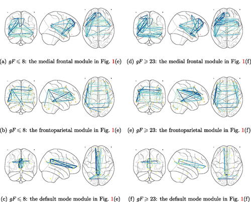However, compared with ${\widehat{\mathbf{\Sigma }}}_{\mathrm{A}},$ the results of ${\widehat{\mathbf{\Sigma }}}_{\mathrm{U}}$ suffer from the heteroscedasticity, as demonstrated in Section 5 and Section E.3 of the supplementary material, and fail to detect any noticeable block structure, hence, we choose not to report them here. To explore the impact of gF on the functional connectivity, we compute the connectivity strength using the standardized form $\left|\right|{\widehat{\Sigma }}_{jk}^{\mathrm{A}}|{|}_{\mathcal{S}}/{(|\left|{\widehat{\Sigma }}_{jj}^{\mathrm{A}}\right|{|}_{\mathcal{S}}\left|\right|{\widehat{\Sigma }}_{kk}^{\mathrm{A}}|{|}_{\mathcal{S}})}^{1/2}$ for $j,k=1\dots ,p.$ Interestingly, we observe from Figure 2 that subjects with $gF\ge 23$ tend to have enhanced brain connectivity in the medial frontal and frontoparietal modules, while the connectivity strength in the default mode module declines. This agrees with existing neuroscience literature reporting a strong positive association between intelligence score and the medial frontal/frontoparietal functional connectivity in the resting state (Van Den Heuvel et al. 2009; Finn et al. 2015), and lends support to the conclusion that lower default mode module activity is associated with better cognitive performance (Anticevic et al. 2012). See also Section E.3 of the supplementary material, in which we illustrate our adaptive functional thresholding estimation using another ADHD dataset.

Fig. 1 Estimated sparsity structures in ${\widehat{\mathbf{\Sigma }}}_{\mathrm{A}}$ using soft functional thresholding rule at fluid intelligence $gF\le 8$ and $gF\ge 23$: (a)–(b) with the corresponding $\widehat{\lambda }$ selected by 5-fold cross-validation; (c)–(f) with the estimated functional sparsity levels set at 70% and 85%.

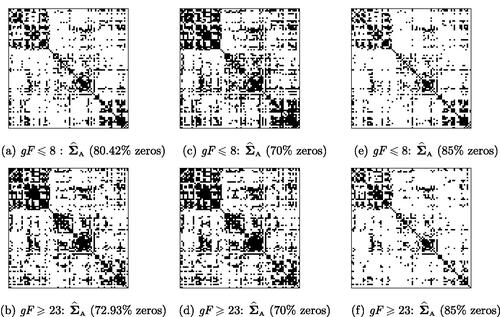
Fig. 2 The connectivity strengths in Figure 1(e)–(f) at fluid intelligence $gF\le 8$ and $gF\ge 23$. Salmon, orange and yellow nodes represent the ROIs in the medial frontal, frontoparietal and default mode modules, respectively. The edge color from cyan to blue corresponds to the value of $\left|\right|{\widehat{\Sigma }}_{jk}^{\mathrm{A}}|{|}_{\mathcal{S}}/{(|\left|{\widehat{\Sigma }}_{jj}^{\mathrm{A}}\right|{|}_{\mathcal{S}}\left|\right|{\widehat{\Sigma }}_{kk}^{\mathrm{A}}|{|}_{\mathcal{S}})}^{1/2}$ from small to large.

Supplementary Materials

The supplementary materials contain all the technical proofs, further methodological derivations and additional discussion and empirical results. We also provide the codes and datasets in Sections 5 and 6 in the supplementary materials.

Acknowledgments

We are grateful to the editor, the associate editor and two referees for their insightful comments and suggestions, which have led to significant improvement of our article.

Disclosure Statement

The authors report there are no competing interests to declare.

Additional information

Funding

Shaojun Guo was partially supported by the National Natural Science Foundation of China (No. 11771447).

References

- Anticevic, A., Cole, M. W., Murray, J. D., Corlett, P. R., Wang, X.-J., and Krystal, J. H. (2012), “The Role of Default Network Deactivation in Cognition and Disease,” Trends in Cognitive Sciences, 16, 584–592. DOI: 10.1016/j.tics.2012.10.008.
- Avella-Medina, M., Battey, H. S., Fan, J., and Li, Q. (2018), “Robust estimation of High-Dimensional Covariance and Precision Matrices,” Biometrika, 105, 271–284. DOI: 10.1093/biomet/asy011.
- Bickel, P. J., and Levina, E. (2008), “Covariance Regularization by Thresholding,” The Annals of Statistics, 36, 2577–2604. DOI: 10.1214/08-AOS600.
- Biswal, B., Zerrin Yetkin, F., Haughton, V. M., and Hyde, J. S. (1995), “Functional Connectivity in the Motor Cortex of Resting Human Brain Using Echo-Planar MRI,” Magnetic Resonance in Medicine, 34, 537–541. DOI: 10.1002/mrm.1910340409.
- Cai, T., and Liu, W. (2011), “Adaptive Thresholding for Sparse Covariance Matrix Estimation,” Journal of the American Statistical Association, 106, 672–684. DOI: 10.1198/jasa.2011.tm10560.
- Cattell, R. B. (1987), Intelligence: Its Structure, Growth and Action, Amsterdam: Elsevier.
- Chang, C., and Glover, G. H. (2010), “Time–Frequency Dynamics of Resting-State Brain Connectivity Measured with fMRI,” Neuroimage, 50, 81–98. DOI: 10.1016/j.neuroimage.2009.12.011.
- Chen, Z., and Leng, C. (2016), “Dynamic Covariance Models,” Journal of the American Statistical Association, 111, 1196–1207. DOI: 10.1080/01621459.2015.1077712.
- Chiou, J.-M., Yang, Y.-F., and Chen, Y.-T. (2016), “Multivariate Functional Linear Regression and Prediction,” Journal of Multivariate Analysis, 146, 301–312. DOI: 10.1016/j.jmva.2015.10.003.
- Fan, J., and Li, R. (2001), “Variable Selection via Nonconcave Penalized Likelihood and its Oracle Properties,” Journal of the American Statistical Association, 96, 1348–1360. DOI: 10.1198/016214501753382273.
- Fan, J., and Marron, J. S. (1994), “Fast Implementations of Nonparametric Curve Estimators,” Journal of Computational and Graphical Statistics, 3, 35–56. DOI: 10.2307/1390794.
- Finn, E. S., Shen, X., Scheinost, D., Rosenberg, M. D., Huang, J., Chun, M. M., Papademetris, X., and Constable, R. T. (2015), “Functional Connectome Fingerprinting: Identifying Individuals Using Patterns of Brain Connectivity,” Nature Neuroscience, 18, 1664–1671. DOI: 10.1038/nn.4135.
- Glasser, M. F., Sotiropoulos, S. N., Wilson, J. A., Coalson, T. S., Fischl, B., Andersson, J. L., Xu, J., Jbabdi, S., Webster, M., Polimeni, J. R. et al. (2013), “The Minimal Preprocessing Pipelines for the Human Connectome Project,” Neuroimage, 80, 105–124. DOI: 10.1016/j.neuroimage.2013.04.127.
- Guo, S., Qiao, X., and Wang, Q. (2022), “Factor Modelling for High-Dimensional Functional Time Series,” arXiv:2112.13651v2 .
- Happ, C., and Greven, S. (2018), “Multivariate Functional Principal Component Analysis for Data Observed on Different (dimensional) Domains,” Journal of the American Statistical Association, 113, 649–659. DOI: 10.1080/01621459.2016.1273115.
- Kong, D., Xue, K., Yao, F., and Zhang, H. H. (2016), “Partially Functional Linear Regression in High Dimensions,” Biometrika, 103, 147–159. DOI: 10.1093/biomet/asv062.
- Kosorok, M. R. (2008), Introduction to Empirical Processes and Semiparametric Inference, Springer Series in Statistics, New York: Springer.
- Lee, K.-Y., Ji, D., Li, L., Constable, T., and Zhao, H. (in press), “Conditional Functional Graphical Models,” Journal of the American Statistical Association, DOI: 10.1080/01621459.2021.1924178.
- Li, B., and Solea, E. (2018), “A Nonparametric Graphical Model for Functional Data with Application to Brain Networks based on fMRI,” Journal of the American Statistical Association, 113, 1637–1655. DOI: 10.1080/01621459.2017.1356726.
- Lotte, F., Bougrain, L., Cichocki, A., Clerc, M., Congedo, M., Rakotomamonjy, A., and Yger, F. (2018), “A Review of Classification Algorithms for EEG-based Brain–Computer Interfaces: A 10 Year Update,” Journal of Neural Engineering, 15, 031005. DOI: 10.1088/1741-2552/aab2f2.
- Miao, R., Zhang, X., and Wong, R. K. (in press), “A Wavelet-based Independence Test for Functional Data with an Application to MEG Functional Connectivity,” Journal of the American Statistical Association, DOI: 10.1080/01621459.2021.2020126.
- Park, J., Ahn, J., and Jeon, Y. (2021), “Sparse Functional Linear Discriminant Analysis, Biometrika, 109, 209–226. DOI: 10.1093/biomet/asaa107.
- Qiao, X., Guo, S., and James, G. (2019), “Functional Graphical Models,” Journal of the American Statistical Association, 114, 211–222. DOI: 10.1080/01621459.2017.1390466.
- Qiao, X., Qian, C., James, G. M., and Guo, S. (2020), “Doubly Functional Graphical Models in High Dimensions,” Biometrika, 107, 415–431. DOI: 10.1093/biomet/asz072.
- Rogers, B. P., Morgan, V. L., Newton, A. T., and Gore, J. C. (2007), “Assessing Functional Connectivity in the Human Brain by fMRI,” Magnetic Resonance Imaging, 25, 1347–1357. DOI: 10.1016/j.mri.2007.03.007.
- Rothman, A. J., Levina, E., and Zhu, J. (2009), “Generalized Thresholding of Large Covariance Matrices,” Journal of the American Statistical Association, 104, 177–186. DOI: 10.1198/jasa.2009.0101.
- Storey, J. D., Xiao, W., Leek, J. T., Tompkins, R. G., and Davis, R. W. (2005), “Significance Analysis of Time Course Microarray Experiments,” Proceedings of the National Academy of Sciences, 102, 12837–12842. DOI: 10.1073/pnas.0504609102.
- Van Den Heuvel, M. P., Stam, C. J., Kahn, R. S., and Pol, H. E. H. (2009), “Efficiency of Functional Brain Networks and Intellectual Performance,” Journal of Neuroscience, 29, 7619–7624. DOI: 10.1523/JNEUROSCI.1443-09.2009.
- Vu, V. Q., and Lei, J. (2013), “Minimax Sparse Principal Subspace Estimation in High Dimensions,” The Annals of Statistics, 41, 2905–2947. DOI: 10.1214/13-AOS1151.
- Wang, H., Peng, B., Li, D., and Leng, C. (2021), “Nonparametric Estimation of Large Covariance Matrices with Conditional Sparsity,” Journal of Econometrics, 223, 53–72. DOI: 10.1016/j.jeconom.2020.09.002.
- Yao, F., Müller, H.-G., and Wang, J.-L. (2005), “Functional Data Analysis for Sparse Longitudinal Data,” Journal of the American Statistical Association, 100, 577–590. DOI: 10.1198/016214504000001745.
- Yuan, M., and Lin, Y. (2006), “Model Selection and Estimation in Regression with Grouped Variables,” Journal of the Royal Statistical Society, Series B, 68, 49–67. DOI: 10.1111/j.1467-9868.2005.00532.x.
- Zapata, J., Oh, S. Y., and Petersen, A. (2022), “Partial Separability and Functional Graphical Models for Multivariate Gaussian Processes, Biometrika, 109, 665–681. DOI: 10.1093/biomet/asab046.
- Zhang, J.-T., and Chen, J. (2007), “Statistical Inferences for Functional Data,” The Annals of Statistics, 35, 1052–1079. DOI: 10.1214/009053606000001505.
- Zhang, X., and Wang, J.-L. (2016), “From Sparse to Dense Functional Data and Beyond,” The Annals of Statistics, 44, 2281–2321. DOI: 10.1214/16-AOS1446.
- Zou, H. (2006), “The Adaptive Lasso and Its Oracle Properties,” Journal of the American Statistical Association, 101, 1418–1429. DOI: 10.1198/016214506000000735.