Ridge Regression Under Dense Factor Augmented Models

Abstract

This article establishes a comprehensive theory of the optimality, robustness, and cross-validation selection consistency for the ridge regression under factor-augmented models with possibly dense idiosyncratic information. Using spectral analysis for random matrices, we show that the ridge regression is asymptotically efficient in capturing both factor and idiosyncratic information by minimizing the limiting predictive loss among the entire class of spectral regularized estimators under large-dimensional factor models and mixed-effects hypothesis. We derive an asymptotically optimal ridge penalty in closed form and prove that a bias-corrected k-fold cross-validation procedure can adaptively select the best ridge penalty in large samples. We extend the theory to the autoregressive models with many exogenous variables and establish a consistent cross-validation procedure using the what-we-called double ridge regression method. Our results allow for nonparametric distributions for, possibly heavy-tailed, martingale difference errors and idiosyncratic random coefficients and adapt to the cross-sectional and temporal dependence structures of the large-dimensional predictors. We demonstrate the performance of our ridge estimators in simulated examples as well as an economic dataset. All the proofs are available in the supplementary materials, which also includes more technical discussions and remarks, extra simulation results, and useful lemmas that may be of independent interest.

KEYWORDS:

• Cross-validation
• High-dimensional linear model
• Mixed-effects model
• Spectral analysis
• Tikhonov regularization

1 Introduction

Improving the bias-variance tradeoff is crucial in many high-dimensional forecasting applications. The classical least-squares regression can suffer from substantial predictive variance when the number of predictors is large compared with the sample size. One useful variance reduction strategy is summarizing massive raw features into a few leading principal components and then predicting the response with these low-dimensional predictors. When the large-dimensional covariates obey a factor structure, the principal component estimator can provide consistent forecasts of the regression function if the factors suffice to predict the target variable. The principal component regression (PCR) often shows better performance than the LASSO regression and ensemble algorithms such as bagging for macroeconomic forecasting; see, for example, Stock and Watson (2002), De Mol, Giannone, and Reichlin (2008), Stock and Watson (2012), Castle, Clements, and Hendry (2013), and Carrasco and Rossi (2016). The PCR is also widely used when studying DNA microarrays (Alter, Brown, and Botstein 2000), medical shapes (Cootes et al. 1995), climate (Preisendorfer 1998), robust synthetic control (Agarwal et al. 2021) and many other fields (see Chapter 6 of James et al. 2021). While the PCR model is dense at the variable level (see, e.g., the discussions in Ng 2013), it relies on only low-dimensional principal components in forecasting. However, when many idiosyncratic components are useful, even though each is negligible, the PCR is not optimal and leaves room for improvement in many empirical applications.

Consider a toy example with $p=100$ covariates $x_i={(x_{i,1},\dots ,x_{i,p})}^{\prime }\in {\mathbb{R}}^p$, where we denote the transpose of any matrix or vector A by $A^{\prime }$, and $n=100$ observations from a factor model given by (1.1) $$x_i={\Lambda }_1{f}_{i,1}+{\Lambda }_2{f}_{i,2}+e_i,\hspace{1em}i=1,\dots ,n.$$(1.1)

The latent factors $f_{i,1}\in \mathbb{R}$ and $f_{i,2}\in \mathbb{R}$, the entries of idiosyncratic variables $e_i={(e_{i,1},\dots ,e_{i,p})}^{\prime }$, and the entries of loading coefficients ${\Lambda }_1={({\Lambda }_{1,1},\dots ,{\Lambda }_{p,1})}^{\prime }$ and ${\Lambda }_2={({\Lambda }_{1,2},\dots ,{\Lambda }_{p,2})}^{\prime }$ are all generated independently from the standard normal distribution. One may think of the data vector $x_i$ as a set of economic variables at a given time. We then generate the target variables $y_i$ from a factor-augmented predictive regression model given by (1.2) $$y_i=0.6f_{i,1}+0.2f_{i,2}+e_i^{\prime }\beta +{\epsilon }_i=:{\mu }_i+{\epsilon }_i,$$(1.2) where the regression errors ${\epsilon }_i$ are generated from the standard normal distribution independently of the regression means ${\mu }_i$. We generate the direction of the coefficient vector $\beta ={({\beta }_1,\dots ,{\beta }_p)}^{\prime }$ uniformly over the ${\mathbb{R}}^p$ unit sphere, and thus each entry ${\beta }_i$ is stochastically negligible for large p. Then we scale the total idiosyncratic signal ${\Vert \beta \Vert }^2={\sum }_{i=1}^p{\beta }_i^2$ through the grid $\{0,0.1,\dots ,1\}$. The PCR model is the special case with ${\Vert \beta \Vert }^2=0$. The idiosyncratic information, at aggregate level, becomes more important as ${\Vert \beta \Vert }^2$ increases.

We plot the median, over 5000 replications, of the training predictive loss $n^{-1}{\sum }_{i=1}^n{({\mu }_i-{\widehat{\mu }}_i)}^2$ as a function of idiosyncratic signal length ${\Vert \beta \Vert }^2$ on the left-hand-side of Figure 1, where ${\mu }_i$ and ${\widehat{\mu }}_i$ denote the population and estimated means of the target variable $y_i$, respectively. We consider both the oracle PCR estimator using the true number of factors $r=2$, and the feasible PCR estimator using a number of PCs selected by 5-fold cross-validation. We compare these PCR estimators with the ridge regression estimator, hereinafter abbreviated as RR estimator, that uses all the raw variables $x_i$ and does not require selecting the number of factors. We select the ridge penalty using 5-fold cross-validation. The median predictive loss of the PCR estimators grows (almost) linearly in the idiosyncratic signal length ${\Vert \beta \Vert }^2$, but that of the RR estimator grows significantly slower. The cross-validated RR estimator is only slightly worse than the oracle PCR estimator but comparable to the cross-validated PCR estimator for small ${\Vert \beta \Vert }^2$, whereas the advantage of RR estimator emerges quickly as ${\Vert \beta \Vert }^2$ grows.

Figure 1: Median predictive loss (left) and change in median sample variance of estimated means (right) as functions of idiosyncratic signal ${\Vert \beta \Vert }^2$.

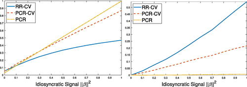
To illustrate the sensitivity of RR to the idiosyncratic information, we plot the median of the sample variance of the estimated means (which equals to the sum of squared estimated coefficients on all standardized components) over the replications on the right-hand-side of Figure 1. To emphasize the changes, we only plot the differences to the values for ${\Vert \beta \Vert }^2=0$. The variance of RR estimates grow quickly with ${\Vert \beta \Vert }^2$, while that of the oracle PCR coefficients hardly change. The cross-validation selection improves the sensitivity of PCR to ${\Vert \beta \Vert }^2$ only slightly because a few extra components are actually asymptotically negligible in our dense models.

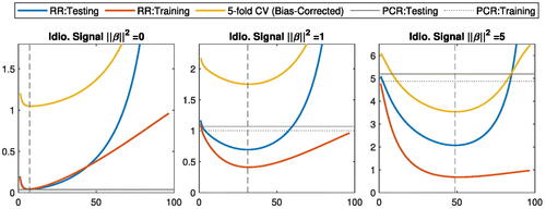
Figure 2 compares the training and testing predictive losses for ridge regression, averaged over 1000 replications, as functions of the effective degrees of freedom (see Hastie, Tibshirani, and Friedman 2009, p. 64) implied by the ridge penalty. We define testing predictive loss as the expected squared forecast error of the out-of-sample regression mean ${\mu }_{\text{oos}}=f_{\text{oos}}^{\prime }\theta +e_{\text{oos}}^{\prime }\beta$ with new variables $f_{\text{oos}}$ and $e_{\text{oos}}$ using the estimated regression function and the new covariates $x_{\text{oos}}$, where $\theta ={(0.6,0.2)}^{\prime }$ and $\beta$ are the population coefficients in (1.2). Again, the optimal ridge estimator (dashed line) for testing predictive loss matches the performance of PCR when ${\Vert \beta \Vert }^2=0$ but outperforms PCR when ${\Vert \beta \Vert }^2>0$. More importantly, these plots illustrate an important relation between training and testing predictive losses for performance evaluation: they share (almost) the same optimal ridge penalty. We formally establish this universal property in Section 2 using a general notation of predictive loss, and generalize the results to time series data in Section 3.

Figure 2: Average training and testing predictive losses for RR and Oracle PCR.

Our toy example illustrates that omitting idiosyncratic information can lead to nontrivial loss in predictive efficiency, and the ridge regression is more robust against PCR capturing both factor and idiosyncratic information. The contribution of this article is a comprehensive theory of the optimality, robustness, and cross-validation consistency of the ridge regression under a general factor-augmented regression model given by (1.3) $$X= F{\Lambda }^{\prime }+E{\Gamma }^{\prime }$$(1.3) (1.4) $$Y= F\theta +E\beta +ϵ$$(1.4) where the left-hand side of the equations represent a large sample of observations in high dimensions: $X={[x_1-\overline{x},\dots ,x_n-\overline{x}]}^{\prime }\in {\mathbb{R}}^{n\times p}$ is the demeaned design matrix of predictors $x_i\in {\mathbb{R}}^p$ with large n and p, and $Y={(y_1-\overline{y},\dots ,y_n-\overline{y})}^{\prime }$ is the demeaned vector of univariate targets $y_i$. Throughout, $\overline{a}=\frac{1}{n}{\sum }_{i=1}^n{a}_i$ denotes the sample mean of any variable a. The low-rank matrix $F={[f_1-\overline{f},\dots ,f_n-\overline{f}]}^{\prime }$ collects low-dimensional latent factors $f_i\in {\mathbb{R}}^r$, r finite, and $E={[e_1-\overline{e},\dots ,e_n-\overline{e}]}^{\prime }$ is a large-dimensional random matrix of idiosyncratic components $e_i\in {\mathbb{R}}^p$. The matrix $\Gamma$ is a rotation matrix, possibly unknown. The fixed-effects $\theta ={({\theta }_1,\dots ,{\theta }_r)}^{\prime }$ on the factors and the random-effects $\beta ={({\beta }_1,\dots ,{\beta }_p)}^{\prime }$ on the idiosyncratic components are both unknown. The noise component $ϵ={({\epsilon }_1-\overline{\epsilon },\dots ,{\epsilon }_n-\overline{\epsilon })}^{\prime }$ is a demeaned vector of uncorrelated (but possibly dependent) regression errors ${\epsilon }_i$. One may also interpret (1.3) and (1.4) as an error-in-variables regression model (6.1) but we postpone the discussions to Section 6.

Many datasets support the low-rank perturbation form (1.3); see the survey by Johnstone and Paul (2018) for many examples in electrocardiogram tracing, microarrays, satellite images, medical shapes, climate, signal detection, and finance. We assume that the low-rank $p\times r$ coefficient matrix $\Lambda =[{\Lambda }_1,\dots ,{\Lambda }_r]$ has a divergent strength $a_p=\mathrm{tr}({\Lambda }^{\prime }\Lambda )\to \infty$ at an arbitrary rate to separate the spectrum of the factor component $F{\Lambda }^{\prime }$ from the stochastically bounded spectrum of the idiosyncratic component $E{\Gamma }^{\prime }$ in (1.3). Therefore, we can analyze the spectral regularization using the standard eigenbasis without suffering from PCA inconsistency issues (Paul 2007; Johnstone and Lu 2009; Onatski 2012). Following Cai, Han, and Pan (2020), we allow the unobservable idiosyncratic components to enter the factor model (1.3) subject to a possibly unknown rotation $\Gamma \in {\mathbb{R}}^{p\times p}$ for generality. We discuss the possibility of extending our results for $a_p=O(1)$, especially when PCA becomes inconsistent, as future works in Appendix A.9 in the supplementary materials.

Our regression model (1.4) is the factor-augmented model proposed by Kneip and Sarda (2011). Substituting $E{\Gamma }^{\prime }=X-F{\Lambda }^{\prime }$ under model (1.3) and using the identity ${\Gamma }^{\prime }\Gamma =I_p$, we can reparameterize the regression model (1.4) as follows: (1.5) $$Y=F\underset{¯}{\theta }+X\underset{¯}{\beta }+ϵ,\hspace{1em}\underset{¯}{\beta }=\Gamma \beta , \underset{¯}{\theta }=\theta -{\Lambda }^{\prime }\underset{¯}{\beta },$$(1.5) where the entries of $\underset{¯}{\theta }$ and $\underset{¯}{\beta }$ are called common and specific effects, respectively. One might also interpret the last equation as a misspecified model where we only observe the design matrix X but not the latent factor matrix F. Throughout the article, we refer factor-augmented regression models to these two equivalent representations (1.4) and (1.5) exchangeably. Note that our model augments the purely variable-based model (with $\underset{¯}{\theta }=\theta -{\Lambda }^{\prime }\Gamma \beta ={(0,\dots ,0)}^{\prime }$) in, for example, Castle, Clements, and Hendry (2013), Fan, Ke, and Wang (2020) by adding extra factor information.

Unlike the aforementioned papers, we study the cases where the coefficient vector $\underset{¯}{\beta }$ is possibly dense. Even if the true regression vector $\beta$ on the idiosyncratic components is sparse, the regression vector $\underset{¯}{\beta }$ on the variables may contain little (or even no) zero entries due to a nontrivial rotation $\Gamma$. In general, we are interested in the models that are possibly dense at both variable and principal component levels. We consider every idiosyncratic component to be asymptotically negligible but allow them to have nontrivial aggregate explanatory power; see Jolliffe (1982), Dobriban and Wager (2018), Giannone, Lenza, and Primiceri (2021), Hastie et al. (2022), and many references therein for examples of applications.

Based on spectral analysis of large-dimensional random matrices, this article shows that the ridge regression is optimal in capturing factor and idiosyncratic information simultaneously among the entire class of spectral regularized estimators under the mixed-effects hypothesis. Ridge regression has a long tradition in statistics tracing back at least to Tikhonov (1963a, 1963b) and Hoerl and Kennard (1970); see Liu and Dobriban (2020) for an excellent survey. To our knowledge, we are the first to study the ridge regression model with factor augmentation. Our analysis of large-dimensional covariance matrices under factor models requires a different approach from that in Dicker (2016) and Dobriban and Wager (2018). In particular, our results extend to more general data generating processes of covariates by analyzing limiting predictive loss instead of predictive risk (i.e., the expected predictive loss); see Appendix A.1 in the supplementary materials for comparisons with Dobriban and Wager (2018).

We prove that the k-fold cross-validation selects the asymptotically optimal ridge penalty, as illustrated in Figure 2, subject to a straightforward bias correction. The bias-corrected selection is uniformly consistent for all positive ridge penalties bounded away from zero, including those diverging to infinity. We extend the scope of the k-fold cross-validation to non-iid data and provide theoretical guarantee for dealing with martingale difference regression errors. Furthermore, we propose a new method called “double” ridge regression and an asymptotically correct k-fold cross-validation method in the presence of nuisance variables, in particular autoregressors, under mild conditions.

The rest of the article is organized as follows. We develop the asymptotic theories for independent errors in Section 2 and then generalize the results to martingale difference errors and autoregressive models in Section 3. More simulated and real-life examples are discussed in Sections 4 and 5, respectively. We conclude the article in Section 6. All the proofs of the theorems are postponed to the supplementary materials. The supplementary materials also provides more technical discussions and remarks about the conditions and auxiliary results, together with additional simulation results and some important lemmas that may be of independent interest.

2 Main Results

First, consider the factor model (1.3) in introduction. We are interested in the asymptotic regime where the number of predictors is comparable to the sample size:

Assumption 1

(Large-dimensional Asymptotics).

The number of covariates $p=p(n)$ and the sample size n are comparable in such a way that $p/n\to c\in (0,\infty )$ as $n\to \infty$.

The concentration ratio $p/n$, possibly larger than 1, plays a central role in our asymptotic theory. Unless specified otherwise, all asymptotic results hold as $n,p\to \infty$ simultaneously in the probability space, enlarged if necessary, with the largest sigma-algebra.

Without loss of generality, we treat both the in-sample factor scores matrix F and the loading matrix $\Lambda$ in (1.3) as fixed parameters. When factors are random, our approach is equivalent to conditioning on a particular realization of F. The number of factors r is finite but not necessarily known.

Assumption 2

(Factor Model).

The following conditions hold:

1. The total factor loading $a_p:=\text{tr}({\Lambda }^{\prime }\Lambda )\to \infty$, and $a_p=O(p)$.

2. (b) ${\Sigma }_{\Lambda }:={\Lambda }^{\prime }\Lambda /a_p$ converges to some $r\times r$ diagonal matrix with diagonal elements ${\sigma }_{ii}\ge {\sigma }_{jj}>0$ for $i<j$. Without loss of generality, $F^{\prime }F/n=I_r$ and ${\Gamma }^{\prime }\Gamma =I_p$ where $I_d$ denotes $d\times d$ identity matrix.

3. (c) ${\lambda }_{\max }({\Omega }_E)=O_{\mathbb{P}}(1)$ where ${\Omega }_E=\frac{1}{n}{E}^{\prime }E$ is the (unobservable) sample covariance matrix of the idiosyncratic components.

Conditions (a)–(c) are the weaker factor models in Bai and Ng (2021) allowing an arbitrarily slow rate of total factor strength $a_p$. When all entries, say, of the loading matrix $\Lambda =\{\Lambda (i,j)\}$ are bounded away from infinity, we readily have $a_p={\sum }_{i=1}^p{\sum }_{j=1}^r{\Lambda }^2(i,j)=O(pr)=O(p)$ in condition (a). We allow the loading matrix $\Lambda$ to have many vanishing entries and one may use $a_p\propto p^{\alpha }$ for any $\alpha \in (0,1]$; see, for example, Bai (2003), Hallin and Liska (2007), and Agarwal et al. (2021) for the linear case $\alpha =1$ and Onatski (2009) for the case $\alpha >2/3$. Via the factor decomposition (1.3) of $X=F{\Lambda }^{\prime }+E{\Gamma }^{\prime }$, these conditions ensure that singular values of the factor part $F{\Lambda }^{\prime }$ to be much larger than (hence, separated from) those of the idiosyncratic part $E{\Gamma }^{\prime }$; see, for example, Cai, Han, and Pan (2020) for discussions and comparisons with the generalized spiked model in Johnstone (2001).

Remarkably, our condition (b) relaxes some identification conditions in the previous papers. We allow ties in the proportion of total loading $\{{\sigma }_{ii}:i=1,\dots ,r\}$ and require only the subspace consistency of PCA in the spirit of Jung and Marron (2009). When there are ties, all bases of the span of corresponding latent factors satisfy our conditions and therefore we are not able to identify the true ones in the data generating process. Nevertheless, we could estimate the subspace as a whole consistently and unify the further factor analysis for cross-validation and autoregressive models, as train-test splits and residual-based estimation can make latent factors indistinguishable in subsamples or after projections. One limitation of condition (b) is that all eigenvalues of $\Lambda$ must diverge at the same rate of $a_p$, but we can easily relax this requirement and allow different rates if necessary.

Condition (c) holds for a separable random matrix $E=B^{1/2}\varsigma A^{1/2}$ in (1.3) where $A\in {\mathbb{R}}^{p\times p}$ and $B\in {\mathbb{R}}^{n\times n}$ are positive-definite matrices with bounded spectral norms and $\varsigma =\left\{{\varsigma }_{ij}\right\}\in {\mathbb{R}}^{n\times p}$ is a random matrix of iid standardized entries with a bounded fourth moment; see, for example, Paul and Silverstein (2009) and Chapter 5 of Bai and Silverstein (2010). Condition (c) also holds for high-dimensional linear time series satisfying the conditions in Remark 8 of Onatski and Wang (2021). See Appendix A.2 of the supplementary materials for more detailed discussions.

For out-of-sample analysis, we assume that the data obeying (1.3) and (1.4) are from the following data generating process (DGP): (2.1) $$\begin{array}{cc}{x}_i=\hfill & \Lambda f_i+\Gamma e_i,\hfill \end{array}$$(2.1) (2.2) $$y_i={\varphi }_0+f_i^{\prime }\theta +e_i^{\prime }\beta +{\epsilon }_i.$$(2.2) where ${\varphi }_0={\varphi }_0(n)$ is an unspecified intercept possibly indexed by n and the regression errors ${\epsilon }_i$ satisfy the following condition:

Assumption 3

(Independent Errors).

The regression errors $\left\{{\epsilon }_i\right\}$ are mutually independent with zero mean $\mathbb{E}{\epsilon }_i=0$ and a common variance ${\sigma }^2=\mathbb{E}{\epsilon }_i^2$ bounded away from zero and infinity, and they are independent of $\{f_i,e_i\}$. They are uniformly integrable in second moment such that $\underset{i\in \mathbb{Z}}{\sup }\mathbb{E}|{\epsilon }_i{|}^{2+2\iota }$ is bounded away from infinity for some $\iota >0$.

This assumption is common in statistical learning literature. We will relax it to handle uncorrelated but dependent errors in Section 3. See also Remark 2 for the relaxation of the homoscedasticity condition. We consider strongly exogenous predictors $\left\{x_i\right\}$ to allow for a standard factor estimation using the entire sample of raw predictors as in, for example, Stock and Watson (2012).

Throughout the article, we consider a mixed-effects model where the factor coefficients $\theta$ are arbitrary fixed-effects and the entries of idiosyncratic coefficient vector $\beta$ are stochastic. In particular, we make the following assumption throughout the article for $\beta ={({\beta }_1,\dots ,{\beta }_p)}^{\prime }$:

Assumption 4

(Random Effects).

The idiosyncratic coefficient vector $\beta =\tau p^{-1/2}b$, where $b={(b_1,\dots ,b_p)}^{\prime }$ is independent of the predictors $\left\{x_i\right\}$ and the regression errors $\left\{{\epsilon }_i\right\}$, and has uncorrelated entries such that $$\mathbb{E}\left[b_i\mid b_j,j\ne i\right]=0, \mathbb{E}\left[b_i^2\mid b_j,j\ne i\right]=1,$$and ${\max }_{1\le i\le p}\mathbb{E}{b}_i^{2+2\iota }$ is bounded away from infinity for some $\iota >0$. The total idiosyncratic signal length ${\tau }^2={\tau }_n^2$ is unknown, possibly dependent on $\left\{x_i\right\}$, and ${\tau }^2=O_{\mathbb{P}}(1)$. When ${\tau }^2=0$, the augmented model (2.2) reduces to the principal component regression model.

This condition is based on the hypothesis of the random effect in, for example, Dobriban and Wager (2018), but here we relax the dependence structure between the entries ${\beta }_i$ and allow them to be non-identically distributed. See Appendix A.3 in the supplementary materials for more examples and comparisons. We emphasize that this assumption is only needed for modeling the idiosyncratic coefficients $\beta$, and we allow for arbitrary fixed-effects $\theta$ on the latent factors in our factor-augmented model (2.2).

We split our main results into two sections: the first one shows the efficiency of the ridge regression among the general class of spectral regularized estimators; the second one establishes the uniform consistency of the bias-corrected k-fold cross-validation for selecting the best ridge penalty.

2.1 On the Optimality of Ridge Regression

In this section, we show that the ridge regression is asymptotically optimal among the spectral regularized estimators in capturing idiosyncratic information and it is more robust than principal component regression against factor augmentation.

Consider the singular value decomposition $n^{-1/2}X={\sum }_{i=1}^K{\lambda }_i^{1/2}{u}_i{v}_i^{\prime }$, where ${\lambda }_i$ denotes the ith largest eigenvalue (counting multiplicities) and $K\le \{n-1,p\}$ denotes the rank of X. Note that $\left\{u_i\right\}$ are all orthogonal to the n-dimensional unit vector proportional to the all-ones vector, denoted by ${\iota }_n:=n^{-1/2}{(1,\dots ,1)}^{\prime }\in {\mathbb{R}}^n$, due to data centering. To reduce the estimation variance of regression means $\mu =F\theta +E\beta$ in (1.4), we shrink the projections of the (uncentered) target vector $y:={(y_1,\dots ,y_n)}^{\prime }\in {\mathbb{R}}^n$ onto the eigenbasis $\left\{{\iota }_n\right\}\cup \{u_i\in {\mathbb{R}}^n:1\le i\le K\}$ via a shrinkage function $\delta :(0,\infty )\to [0,1]$: (2.3) $$\widehat{\mu }(\delta )={\iota }_n{\iota }_n^{\prime }y+\sum _{i=1}^K\delta ({\lambda }_i)u_i{u}_i^{\prime }y={({\widehat{m}}_{\tilde{\delta }}(x_1),\dots ,{\widehat{m}}_{\tilde{\delta }}(x_n))}^{\prime }$$(2.3) where ${\widehat{m}}_{\tilde{\delta }}$ is the estimated regression function given by (2.4) $${\widehat{m}}_{\tilde{\delta }}(x)=\overline{y}+{(x-\overline{x})}^{\prime }\widehat{\beta }(\tilde{\delta }),$$(2.4) and $\widehat{\beta }(\tilde{\delta })$ is a penalized least-squares estimator (Tikhonov 1963a, 1963b) given by (2.5) $$\widehat{\beta }(\tilde{\delta })={\left(X^{\prime }X+nW(\tilde{\delta })\right)}^{+}{X}^{\prime }Y$$(2.5)

with $A^{+}$ denoting the Moore-Penrose inverse of any matrix A and the weight matrix (2.6) $$W(\tilde{\delta })=\sum _{i=1}^K\tilde{\delta }({\lambda }_i)v_i{v}_i^{\prime },\hspace{1em}\tilde{\delta }(x)=x\cdot \frac{1-\delta (x)}{\delta (x)}.$$(2.6)

In particular, choosing $\tilde{\delta }(x)\equiv \gamma$ and $\delta (x)=\frac{x}{x+\gamma }$ for some constant $\gamma >0$ in (2.5) yields the ridge (Hoerl and Kennard 1970) estimator $\widehat{\beta }(\gamma )={(X^{\prime }X+n\gamma I_p)}^{-1}{X}^{\prime }Y$. We allow for infinite penalties for dimension reduction purpose: one should interpret $\tilde{\delta }(x)=\infty$ if and only if $\delta (x)=0$, and then we must set $\beta$ orthogonal to $v_i$ in estimation. For more discussions we refer to Hastie, Tibshirani, and Friedman (2009, chap. 3). Henceforth we call (2.3) a spectral regularized estimator of the regression means.

We define the predictive loss as the reducible mean squared forecast error (see James et al. 2021 for decomposition into reducible and irreducible errors), conditional on a realization of the training set, given by $$\tilde{L}(\delta )=\mathbb{E}\left[{\left({\mu }_{\text{oos}}-{\widehat{m}}_{\tilde{\delta }}(x_{\text{oos}})\right)}^2\mid {\mathcal{S}}_n\right],$$where $x_{\text{oos}}=\Lambda f_{\text{oos}}+\Gamma e_{\text{oos}}$ and ${\mu }_{\text{oos}}={\varphi }_0+f_{\text{oos}}^{\prime }\theta +e_{\text{oos}}^{\prime }\beta$ are out-of-sample (OOS) random covariates and the regression mean from the DGPs (2.1) and (2.2) with the same factor model parameters and regression coefficients. The sigma-algebra ${\mathcal{S}}_n$ is generated by the in-sample variables $\{f_i,e_i,{\epsilon }_i:i\le n\}$ and the random coefficients $\beta$.

We use the following paradigm to evaluate the spectral regularized estimators.

Assumption 5

(Evaluation Paradigm).

The new variables $f_{\text{oos}}$ and $e_{\text{oos}}$ are independent of both in-sample regression errors $\{{\epsilon }_i:i\le n\}$ and random coefficients $\beta$, given the in-sample random variables $\{f_i,e_i:i\le n\}$. The conditional covariance matrices of $a_{\text{oos}}$ centered around the sample mean given by ${\tilde{\Omega }}_a=\mathbb{E}[(a_{\text{oos}}-\overline{a}){(a_{\text{oos}}-\overline{a})}^{\prime }|{\mathcal{S}}_n]$ have spectral norms bounded in n for both $a\in \{f,e\}$.

This paradigm is flexible enough to include both the training and testing predictive losses used in Figure 2:

• If one draws the pair of new variables $f_{\text{oos}}$ and $e_{\text{oos}}$ uniformly over the sample $\{f_i,e_i:1\le i\le n\}$, then we obtain the training predictive loss given by (2.7) $$\tilde{L}(\delta )=\frac{1}{n}\sum _{i=1}^n{({\mu }_i-m_{\tilde{\delta }}(x_i))}^2=\frac{1}{n}{\Vert \mu -\widehat{\mu }(\delta )\Vert }^2,$$(2.7) with the sample covariance matrices ${\tilde{\Omega }}_a=\frac{1}{n}{\sum }_{i=1}^n(a_i-\overline{a}){(a_i-\overline{a})}^{\prime }$ for $a\in \{f,e\}$.

• A more typical implementation is to generate $f_{\text{oos}}$ and $e_{\text{oos}}$, independent of ${\mathcal{S}}_n$, from some population distribution or a random draw on a test set in order to assess the testing predictive loss. Then ${\tilde{\Omega }}_a={\Sigma }_a+({\mu }_a-\overline{a}){({\mu }_a-\overline{a})}^{\prime }$, where ${\mu }_a$ and ${\Sigma }_a$ denote the mean and covariance matrix of $a_{\text{oos}}$ for $a\in \{f,e\}$.

Our estimated regression function (2.4) uses oracle estimators ${\Lambda }^{\prime }\widehat{\beta }(\tilde{\delta })$ and ${\Gamma }^{\prime }\widehat{\beta }(\tilde{\delta })$ of $\theta$ and $\beta$, respectively via the decomposition: $${\widehat{m}}_{\tilde{\delta }}(x_{\text{oos}})=\overline{y}+{(f_{\text{oos}}-\overline{f})}^{\prime }{\Lambda }^{\prime }\widehat{\beta }(\tilde{\delta })+{(e_{\text{oos}}-\overline{e})}^{\prime }{\Gamma }^{\prime }\widehat{\beta }(\tilde{\delta }).$$

The following theorem relates $\tilde{L}(\delta )$ to the estimation error of linear coefficients and gives further stochastic approximations based on spectral analysis.

Theorem 1.

Under Assumptions 1–5, for any sequence of candidate shrinkage function $\delta ={\delta }_n:(0,\infty )\to [0,1]$ may or may not depend on the covariates in the training set, (2.8) $$\tilde{L}(\delta )-{\Vert \theta -{\Lambda }^{\prime }\widehat{\beta }(\tilde{\delta })\Vert }_{{\tilde{\Omega }}_f}^2-{\Vert \beta -{\Gamma }^{\prime }\widehat{\beta }(\tilde{\delta })\Vert }_{{\tilde{\Omega }}_e}^2\stackrel{\mathbb{P}}{\to }0,$$(2.8)

where ${\Vert v\Vert }_{\Omega }^2=v^{\prime }\Omega v$ denotes the weighted norm of any vector v. Furthermore, (2.9) $${\Vert \theta -{\Lambda }^{\prime }\widehat{\beta }(\tilde{\delta })\Vert }_{{\tilde{\Omega }}_f}^2-{\theta }^{\prime }{D}_{\delta }{\tilde{\Omega }}_f{D}_{\delta }\theta \stackrel{\mathbb{P}}{\to }0,$$(2.9) (2.10) $$\begin{array}{c}{\Vert \beta -{\Gamma }^{\prime }\widehat{\beta }(\tilde{\delta })\Vert }_{{\tilde{\Omega }}_e}^2-{\int }_0^{{\lambda }_{r+1}}\left\{{\tau }^2{(1-\delta (x))}^2+{\sigma }^2\frac{p}{n}\frac{{\delta }^2(x)}{x}\right\}d{\tilde{F}}_p(x)\\ -{\tau }^2{\tilde{F}}_p(0)\stackrel{\mathbb{P}}{\to }0.\end{array}$$(2.10) where $D_{\delta }=\mathrm{diag}(1-\delta ({\lambda }_1),\dots ,1-\delta ({\lambda }_r))$ and ${\tilde{F}}_p(x)=\frac{1}{p}{\sum }_{i=1}^p{v}_i^{\prime }\Gamma {\tilde{\Omega }}_e{\Gamma }^{\prime }{v}_{i}1({\lambda }_i\le x)$, if there is no tie values in $\{{\sigma }_{ii}:i=1,\dots ,r\}$ and the penalty function $\tilde{\delta }$ is bounded away from 0. The probability mass ${\tilde{F}}_p(0)>0$ when the data matrix X is column-rank deficient with $p>n$. More generally, the result remains true if $\delta ({\lambda }_i)=\delta ({\lambda }_j)+o_{\mathbb{P}}(1)\stackrel{\mathbb{P}}{\to }0$ for every tie values ${\sigma }_{ii}={\sigma }_{jj}$ with $1\le i<j\le r$.

The estimation errors of fixed and random effects are asymptotically orthogonal in (2.8) because their interaction vanishes through aggregation of the uncorrelated mean-zero random coefficients and regression errors. Via the approximation (2.8) one can interpret different predictive loss functions using different weight matrices: (a) the training errors weight the coefficient estimation errors by the sample covariance matrices; (b) the testing errors weight the coefficient estimation errors by the population covariance matrices (centered around sample means); (c) the $L_2$ norm of coefficient estimation error ${\Vert \theta -{\Lambda }^{\prime }\widehat{\beta }(\tilde{\delta })\Vert }^2+{\Vert \beta -{\Gamma }^{\prime }\widehat{\beta }(\tilde{\delta })\Vert }^2$ uses identity weight matrices ${\tilde{\Omega }}_a=I_p$ for $a\in \{f,e\}$. The asymptotic limit in (2.9) shows the bias of shrinkage estimator of fixed-effects $\theta$, and that in (1) shows the bias-variance tradeoff for random-effects estimation.

Remark 1

(PCR).

Plugging in the shrinkage function $\delta (x)=1[x>{\lambda }_{r+1}]$ for the oracle PCR estimator yields a limit increasing linearly in ${\Vert \beta \Vert }^2$ as depicted in Figure 1: $$\begin{array}{cc}\tilde{L}\left(\delta \right)\hfill & =0\cdot {\Vert \theta \Vert }^2+{\int }_0^{{\lambda }_{r+1}}\left\{{\tau }^2{(1-0)}^2+{\sigma }^2\frac{p}{n}\frac{0^2}{x}\right\}d{\tilde{F}}_p(x)\hfill \\ \mathrm{\hspace{1em}}\mathrm{\hspace{1em}}+{\tau }^2{\tilde{F}}_p(0)+o_{\mathbb{P}}(1)\hfill & \hfill \\ ={\tau }^2{\tilde{F}}_p({\lambda }_{r+1})+o_{\mathbb{P}}(1)={\Vert \beta \Vert }^2\cdot \frac{1}{p}\text{tr}({\tilde{\Omega }}_e)+o_{\mathbb{P}}(1)\hfill & \hfill \end{array}$$where the last equation is due to the facts that ${\Vert \beta \Vert }^2={\tau }^2+o_{\mathbb{P}}(1)$ and the random slope ${\tilde{F}}_p({\lambda }_{r+1})=p^{-1}\text{tr}({\tilde{\Omega }}_e)+o_{\mathbb{P}}(1)$. In fact, this linear pattern generalizes for any PCR estimator using a finite number of $\widehat{r}\ge r$ principal components as adding a few idiosyncratic components does not change its asymptotic behavior in dense models.

Note that the candidate shrinkage function $\delta$ is arbitrary on the positive line as long as it is “honest” in the sense that it only depends on the covariates but not the target variable before selection. Our limit theorem shows that shrinking the projections of the target vector onto the first r principal components can only increase the predictive loss asymptotically via the squared bias (2.9). We should keep the leading principal components unshrunk asymptotically by choosing a shrinkage function such that $1-\delta ({\lambda }_i)\stackrel{\mathbb{P}}{\to }0$ for all $i=1,\dots ,r$ and thus the fixed-effects estimator is consistent in the sense that ${\Vert \theta -{\Lambda }^{\prime }\widehat{\beta }(\tilde{\delta })\Vert }^2\stackrel{\mathbb{P}}{\to }0$.

We will discuss how to choose the optimal (ridge) estimator satisfying this condition later on. Therefore, now we focus on this subset of shrinkage functions and study the limiting predictive loss in the following corollary:

Corollary 1.

Suppose that $1-\delta ({\lambda }_i)\stackrel{\mathbb{P}}{\to }0$ for all $i=1,\dots ,r$. Theorem 1 implies that (2.11) $$\tilde{L}\left(\delta \right)-{\int }_0^{\infty }\left\{{\tau }^2{(1-\delta (x))}^2+{\sigma }^2\frac{p}{n}\frac{{\delta }^2(x)}{x}\right\}d{\tilde{F}}_p(x)-{\tau }^2{\tilde{F}}_p(0)\stackrel{\mathbb{P}}{\to }0,$$(2.11) where we integrate the limiting error over the entire domain of ${\tilde{F}}_p$ for notational convenience although it is asymptotically equivalent to integrate over only the sub-interval $[0,{\lambda }_{r+1}]$.

If further provided that, with probability one, ${\lambda }_{\max }({\tilde{\Omega }}_e)$ is bounded by some absolute constant and ${\tilde{F}}_p$ converges vaguely to a nonrandom limit $\tilde{F}$, then Corollary 1 remain true with ${\tilde{F}}_p$ replaced by the nonrandom limit $\tilde{F}$ for every continuous shrinkage function $\delta$. In particular, we have the following special cases.

Corollary 2.

Let the signal length ${\tau }^2$ and error variance ${\sigma }^2$ be constants, and generate the new variables $e_{\text{oos}}$ independent of the training data. Suppose that all the entries of $e_i$ and $e_{\text{oos}}$ are from an iid array with mean zero and variance ${\sigma }_e^2$. Then, Corollary 1 implies that for every continuous shrinkage functions $\delta$ such that $\underset{x\to \infty }{\lim }\delta (x)=1$, (2.12) $$\tilde{L}\left(\delta \right)\stackrel{\mathbb{P}}{\to }{\int }_0^{\infty }\left\{{\tau }^2{(1-\delta (x))}^2+{\sigma }^{2}c\frac{{\delta }^2(x)}{x}\right\}dF(x)+{\tau }^{2}F(0),$$(2.12)

where F is the Marčenko and Pastur (1967) law with a point mass $F(0)=\max \{0,1-1/c\}$ at the origin, and the positive density function $F^{\prime }(x)=\frac{1}{2\pi xy{\sigma }_e^2}\sqrt{(b-x)(x-a)}$ on [a, b] (and zero density elsewhere) with $a={\sigma }_e^2{(1-\sqrt{c})}^2$ and $b={\sigma }_e^2{(1+\sqrt{c})}^2$. More examples satisfying (2.12) with various limits F are available in Appendix A.4 in the supplementary materials.

For generality, we use the stochastic approximation (2.11) according to the random nature of the predictive loss. We shall show that the optimal (ridge) estimator is asymptotically invariant to the random measure ${\tilde{F}}_p$ (or its limit F if any), and therefore the optimality of ridge regression does not rely on the spectral convergence of large-dimensional covariance matrices.

First, consider the degenerate scenario in that the PCR model is correct with ${\tau }^2=0$, or more generally ${\tau }^2\stackrel{\mathbb{P}}{\to }0$. One may still use a ridge estimator to minimize the limiting error (2.11) with the shrinkage function $\delta (x)=\frac{x}{x+\gamma }$ such that the ridge penalty $\gamma ={\gamma }_n$ is diverging at a slower rate of the smallest spiked value ${\lambda }_r\stackrel{\mathbb{P}}{\to }\infty$. To our knowledge, this finding first appeared formally in De Mol, Giannone, and Reichlin (2008) who studied the PCR model with $a_p$ diverging at a linear rate of p. Such ridge estimator is a smoothed approximation of the PCR estimator performing an asymptotic selection of principal components in the sense that $\delta ({\lambda }_i)=\frac{{\lambda }_i}{{\lambda }_i+\gamma }\ge \frac{{\lambda }_r}{{\lambda }_r+\gamma }\stackrel{\mathbb{P}}{\to }1$ as $\gamma /{\lambda }_r=O_{\mathbb{P}}(\gamma /a_p)\stackrel{\mathbb{P}}{\to }0$ for $i=1,\dots ,r$, while $\delta ({\lambda }_i)=\frac{{\lambda }_i}{{\lambda }_i+\gamma }\le \frac{{\lambda }_{r+1}}{{\lambda }_{r+1}+\gamma }\stackrel{\mathbb{P}}{\to }0$ for all the non-spiked eigenvalues $\{{\lambda }_i:i\ge r+1\}$ that are stochastically bounded as $\gamma \stackrel{\mathbb{P}}{\to }\infty$. In practice, one may select such a ridge penalty coefficient by using cross-validation and we postpone the details to next section. The optimal predictive loss vanishes to zero in probability as we can estimate the fixed-effects consistently and the random-effects are negligible.

A more interesting case is the augmented model with an idiosyncratic signal length ${\tau }^2>0$ bounded away from zero (stochastically), minimizing the asymptotic limit in (2.11) is equivalent to minimizing the integrand $${\tau }^2{(1-\delta (x))}^2+{\sigma }^2\frac{p}{n}\frac{{\delta }^2(x)}{x} \text{for each} x\in (0,\infty ).$$

That is, for each $x\in (0,\infty )$, we choose $\delta (x)$ as the minimum point of the convex quadratic function $${\Delta }_x(\delta ):={\tau }^2{(1-\delta )}^2+{\sigma }^2\frac{p}{n}\frac{{\delta }^2}{x}, \delta \in [0,1].$$

By solving the first-order condition ${\Delta }_x^{\prime }(\delta )=0$, it is elementary to show that the optimal shrinkage function is given by (2.13) $${\delta }^{*}(x)=\frac{x}{x+{\gamma }^{*}},\hspace{1em}{\gamma }^{*}=\frac{p}{n}\frac{{\sigma }^2}{{\tau }^2},\hspace{1em}\Rightarrow \hspace{1em}{\tilde{\delta }}^{*}(x)\equiv {\gamma }^{*}$$(2.13) which corresponds to a ridge estimator with the penalty coefficient ${\gamma }^{*}$, that is, with $W({\tilde{\delta }}^{*})={\gamma }^{*}{I}_p$ in (2.5). One can interpret ${\gamma }^{*}$ as the noise-to-signal ratio ${\sigma }^2/{\tau }^2$ scaled by the aspect ratio $p/n$. Note that the optimal predictive loss is not vanishing in this case as the high-dimensional random-effects $\beta$ cannot be estimated consistently. Since the ridge coefficient ${\gamma }^{*}$ is now (stochastically) bounded, the optimal shrinkage function (2.13) naturally satisfies the conditions that $1-\delta ({\lambda }_i)\stackrel{\mathbb{P}}{\to }0$ as the spiked eigenvalues ${\lambda }_i\stackrel{\mathbb{P}}{\to }\infty$ for $1\le i\le r$, leading to a consistent estimation of the fixed-effects $\theta$.

Remarkably, the optimal shrinkage function (2.13) is the same for all our predictive loss functions sharing the approximate form (2.11). We summarize the optimality of ridge regression into the following corollary:

Corollary 3

(Optimality of ridge regression).

Consider any predictive loss $\tilde{L}$ admitting the asymptotic approximation in Theorem 1. For an arbitrarily small $\zeta >0$ and any candidate shrinkage function $\delta ={\delta }_n$ from Theorem 1, $$\mathbb{P}\left(\tilde{L}\left(\delta \right)>\tilde{L}\left({\delta }^{*}\right)-\zeta \right)\to 1,$$where ${\delta }^{*}(x)=\frac{x}{x+{\gamma }^{*}}$ denotes the shrinkage function for the optimal ridge estimator with the penalty coefficient ${\gamma }^{*}=\frac{p}{n}\frac{{\sigma }^2}{{\tau }^2}$ when ${\tau }^2$ is bounded away from 0 with probability approaching 1, or otherwise an arbitrary diverging penalty ${\gamma }^{*}\stackrel{\mathbb{P}}{\to }\infty$ but ${\gamma }^{*}=o_{\mathbb{P}}(a_p)$ if ${\tau }^2=o_{\mathbb{P}}(1)$. In the latter case, $\tilde{L}({\delta }^{*})\stackrel{\mathbb{P}}{\to }0$ and we may take ${\gamma }^{*}=\hspace{0.17em}\exp \hspace{0.17em}({\sum }_{i=1}^{r_{\max }+1}{w}_i\hspace{0.17em}\log \hspace{0.17em}{\lambda }_i)$ where $w_i\in (0,1)$ are arbitrary fixed weights such that ${\sum }_{i=1}^{r_{\max }+1}{w}_i=1$ for any pre-specified bound $r_{\max }\ge r$. However, in general, only the fixed-effects are consistently estimated in the sense that ${\Vert \theta -{\Lambda }^{\prime }\widehat{\beta }(\tilde{\delta })\Vert }^2\stackrel{\mathbb{P}}{\to }0$ and the optimal ridge estimator trades off the estimation bias and variance of random-effects.

Remark 2.

Corollary 3 generalizes for heteroscedastic errors with different variance ${\sigma }_i^2=\mathrm{var}({\epsilon }_i)$ under more strengthened conditions on the covariates $\left\{x_i\right\}$, where one can relax expression (2.13) by replacing ${\sigma }^2$ with the average variance ${\overline{\sigma }}^2=\frac{1}{n}{\sum }_{i=1}^n{\sigma }_i^2$. Due to the space limit, we postpone the details to Appendix A.8 in the supplementary materials.

2.2 Uniform Consistency of Bias-Corrected k-Fold Cross-Validation

This section establishes the uniform consistency of the k-fold cross-validation (CV) algorithm for selecting the best ridge estimators, subject to a straightforward bias correction. Our asymptotic limits of the cross-validated mean squared error is uniform for all positive ridge penalties bounded away from zero, including those diverging to infinity. Throughout we use a fixed number of folds $k\ge 2$. Generally speaking, there are both computational and statistical advantages to use k-fold CV rather than the leave-one-out CV; see, for example, Section 5.1.3 of James et al. (2021). On the other hand, using a small number of folds may introduce a bias in the selection if the optimal parameter depends on the sample size of the training set.

To fix ideas, the procedure starts from partitioning the entire index sets $\{1,\dots ,n\}$ into k mutually exclusive subsets ${\mathcal{I}}_1,\dots ,{\mathcal{I}}_k$. For generality, we treat the partition $\{{\mathcal{I}}_j:j=1,\dots ,k\}$ as fixed for any given n. When the folds are randomly created, our setup is equivalent to conditioning on a particular realization. One simple choice is to divide $\mathcal{I}$ into blocks, using consecutive indexes in each fold. In general, it is unnecessary to use blocks, and we may assign indexes randomly to the folds. Following the common practice, we generate folds of approximately equal size such that $n_j/n\to 1/k$ where $n_j:=\left|{\mathcal{I}}_j\right|$ denotes the cardinality of the index subset ${\mathcal{I}}_j$.

Let ${\tilde{y}}_i=y_i-\overline{y}$ and ${\tilde{x}}_i=x_i-\overline{x}$ be the demeaned observations, $\overline{y}$ and $\overline{x}$ are the sample means using all data. For any fold ${\mathcal{I}}_j$ treated as a validation set, we fit a ridge estimator ${\widehat{\beta }}_{-j}(\gamma )$ on the remaining $k-1$ folds by minimizing the $L_2$ penalized error given by (2.14) $${\widehat{\beta }}_{-j}(\gamma )=\underset{\beta }{\mathrm{argmin}}\left\{\frac{1}{n_{-j}}\sum _{i\notin {\mathcal{I}}_j}{({\tilde{y}}_i-{\tilde{x}}_i^{\prime }\beta )}^2+\gamma {\Vert \beta \Vert }^2\right\},$$(2.14) where $n_{-j}=n-n_j$ denotes the number of training observations, and $\gamma >0$ is a candidate ridge penalty coefficient. Recall the demeaned design matrix $X={[{\tilde{x}}_1,\dots ,{\tilde{x}}_n]}^{\prime }$ and demeaned target vector $Y={({\tilde{y}}_1,\dots ,{\tilde{y}}_n)}^{\prime }$. Let $D_{-j}=\text{diag}(1[1\in {\mathcal{I}}_{-j}],\dots ,1[n\in {\mathcal{I}}_{-j}])$ be the $n\times n$ diagonal matrices that selects the observations on the training set ${\mathcal{I}}_{-j}:={\mathcal{I}}_j^{\complement }$. Solving the quadratic optimization problem (2.14) yields a close-form solution given by (2.15) $${\widehat{\beta }}_{-j}(\gamma )={\left(X^{\prime }{D}_{-j}X+n_{-j}\gamma I_p\right)}^{-1}{X}^{\prime }{D}_{-j}Y.$$(2.15)

The mean squared error on the observations in the held-out fold ${\mathcal{I}}_j$ is given by $${\text{MSE}}_j(\gamma )=\frac{1}{n_j}\sum _{i\in {\mathcal{I}}_j}({\tilde{y}}_i-{\tilde{x}}_i^{\prime }{\widehat{\beta }}_{-j}(\gamma ){)}^2.$$

We repeat the procedure for $j=1,\dots ,k$, and average these errors to compute the k-fold cross-validation MSE given by $${\text{CV}}^{(k)}(\gamma )=\sum _{j=1}^k\frac{n_j}{n}{\text{MSE}}_j(\gamma )=\frac{1}{n}\sum _{j=1}^k\sum _{i\in {\mathcal{I}}_j}({\tilde{y}}_i-{\tilde{x}}_i^{\prime }{\widehat{\beta }}_{-j}(\gamma ){)}^2.$$

Then we choose the value of $\gamma$ over a sufficiently fine grid that minimizes ${\text{CV}}^{(k)}(\gamma )$. Note that we do not need to estimate the factor scores nor to determine the number of factors with ridge regression.

To apply factor analysis to the training subsamples rather than the full sample, we assume one additional regularity condition:

Assumption 6.

Let ${\Omega }_{f,-j}:=n_{-j}^{-1}\sum _{i\notin {\mathcal{I}}_j}(f_i-\overline{f}){(f_i-\overline{f})}^{\prime }$ denote the training covariance matrix latent factor scores. For every $j=1,\dots ,k$, the eigenvalues of the $r\times r$ matrix ${\Omega }_{f,-j}^{1/2}{\Sigma }_{\Lambda }{\Omega }_{f,-j}^{1/2}$ converge to some limits ${\sigma }_{11,-j}\ge \cdots \ge {\sigma }_{rr,-j}>0$.

The condition allows us to reparameterize the factor scores and loadings on the training set to maintain similar orthogonal structures in Assumption 2. More specifically, consider the spectral decomposition ${\Omega }_{f,-j}^{1/2}{\Sigma }_{\Lambda }{\Omega }_{f,-j}^{1/2}=Q_{-j}{\Sigma }_{-j}{Q}_{-j}^{\prime }$ where ${\Sigma }_{-j}$ is a diagonal matrix and $Q_{-j}$ is an orthogonal matrix. Define the demeaned matrix of the idiosyncratic information $E:={[e_1-\overline{e},\dots ,e_n-\overline{e}]}^{\prime }$. The training design matrix obeys the approximate factor model $$D_{-j}X=D_{-j}F{\Lambda }^{\prime }+D_{-j}E{\Gamma }^{\prime }=F_{-j}{\Lambda }_{-j}^{\prime }+D_{-j}E{\Gamma }^{\prime }$$where $F_{-j}:=D_{-j}F{\Omega }_{f,-j}^{-1/2}{Q}_{-j}$ and ${\Lambda }_{-j}:=\Lambda {\Omega }_{f,-j}^{1/2}{Q}_{-j}$ satisfy the orthogonal conditions: $$\begin{array}{c}{F}_{-j}^{\prime }{F}_{-j}/n_{-j}=I_r,\hspace{1em}\text{and}\\ {\Lambda }_{-j}^{\prime }{\Lambda }_{-j}/a_p={\Sigma }_{-j}\to \text{diag}({\sigma }_{11,-j},\dots ,{\sigma }_{rr,-j}).\end{array}$$

Assumption 6 holds under a stronger condition that $n_{-j}^{-1}\sum _{t\notin {\mathcal{I}}_j}(f_i-\overline{f}){(f_i-\overline{f})}^{\prime }\to I_r$ for all $j=1,\dots ,k$, in which case the limiting eigenvalue ${\sigma }_{ii,-j}={\sigma }_{ii}$. If $f_i$ are iid random vectors with an identity covariance matrix, the conditions holds almost surely by strong law of large numbers. When $\left\{f_i\right\}$ is a (multivariate) time series and the folds are blocks, that is, each time index subset ${\mathcal{I}}_j$ corresponds to a continuous time period, the condition follows from ergodicity: $$\begin{array}{cc}\frac{1}{n_{-j}}\sum _{i\notin {\mathcal{I}}_j}(f_i-\overline{f}){(f_i-\overline{f})}^{\prime }\hfill & =\frac{n}{n_{-j}}\frac{1}{n}\sum _{i=1}^n(f_i-\overline{f}){(f_i-\overline{f})}^{\prime }\hfill \\ \hspace{1em}-\frac{n_j}{n_{-j}}\frac{1}{n_j}\sum _{t\in {\mathcal{I}}_j}(f_i-\overline{f}){(f_i-\overline{f})}^{\prime }\hfill & \hfill \\ =\frac{n}{n_{-j}}{I}_r-\frac{n_j}{n_{-j}}{I}_r+o_{\mathbb{P}}(1)\hfill & \hfill \\ =I_r+o_{\mathbb{P}}(1)\hfill & \hfill \end{array}$$for any stationary ergodic process $\{f_i:i\in \mathbb{Z}\}$ with zero mean and identity covariance matrix, where $\mathbb{Z}$ denotes the set of integers; see Blum and Eisenberg (1975) for more discussions. Assumption 6 then holds with probability approaching 1.

Furthermore, when the folds are randomly generated, the results remain true if the projection process $\{w^{\prime }{f}_i:i\in \mathbb{Z}\}$ is stationary and strong mixing for every unit vectors $w\in {\mathbb{R}}^r$ by combining the theorem in Blum and Hanson (1960) and Cramér–Wold device. See Bradley (1986) and Bradley (2005) for the various types of sufficient conditions for strong mixing.

Theorem 2.

Suppose that Assumptions 1–4 and 6 hold. Uniformly for all positive ridge penalties $\gamma$ bounded away from 0, $$\begin{array}{cc}{\text{CV}}^{(k)}(\gamma )\hfill & -{\sigma }^2-{\left(\frac{\gamma }{a_p+\gamma }\right)}^2\cdot {\theta }^{\prime }{W}_{\gamma }\theta \hfill \\ -{\int }_0^{\infty }\left\{{\tau }^2\frac{{\gamma }^2}{{\left(x+\gamma \right)}^2}+{\sigma }^2\frac{p}{n_{\text{eff}}}\frac{x}{{\left(x+\gamma \right)}^2}\right\}d{F}_p^{(k)}(x)\hfill & \hfill \\ -{\tau }^2{F}_p^{(k)}(0)\stackrel{\mathbb{P}}{\to }0,\hfill & \hfill \end{array}$$

where $F_p^{(k)}$ is some (improper) empirical distribution depending only on the covariates $\left\{x_i\right\}$, the effective training sample size is given by $n_{\text{eff}}=\frac{1}{k}{\sum }_{j=1}^k{n}_{-j}$ provided that $n_j/n$ converges to the same limit for all j, and $W_{\gamma }\in {\mathbb{R}}^{r\times r}$ is a random weight matrix being stochastically bounded and positive-definite with probability tending to 1 when $r>0$. The closed-form expressions of $F_p^{(k)}$ and $W_{\gamma }$ are available in Section E.3 of the supplementary materials.

The first term ${\sigma }^2$ is irreducible but irrelevant to the choice of $\gamma$. The second term ${(\frac{\gamma }{a_p+\gamma })}^2\cdot {\theta }^{\prime }{W}_{\gamma }\theta$ represents the cross-validated estimation error of the fixed-effects at the same (stochastic) order of ${(\frac{\gamma }{a_p+\gamma })}^2{\Vert \theta \Vert }^2$. The rest represents the cross-validated error for the random-effects where we use $n_{\text{eff}}\approx \frac{k-1}{k}n$ due to the train-test split.

Let ${\widehat{\gamma }}_{\text{cv}}$ denote the optimal ridge penalty selected by the regular k-fold CV. When ${\tau }^2\stackrel{\mathbb{P}}{\to }0$, the k-fold CV chooses some divergent penalty ${\widehat{\gamma }}_{\text{cv}}\stackrel{\mathbb{P}}{\to }\infty$ to shrink the random-effects estimator toward zero as much as possible but ${\widehat{\gamma }}_{\text{cv}}=o_{\mathbb{P}}(a_p)$ (unless ${\Vert \theta \Vert }^2=0$) such that the fixed-effect estimation errors vanish as well. Note that any divergent penalty sequence proportional to ${\widehat{\gamma }}_{\text{cv}}$ is also asymptotically optimal. When ${\tau }^2$ is bounded away from 0, by the same arguments above Corollary 3, one should again minimize the integrand ${\tau }^2\frac{{\gamma }^2}{{(x+\gamma )}^2}+{\sigma }^2\frac{p}{n_{\text{eff}}}\frac{x}{{(x+\gamma )}^2}$ by using the optimal penalty ${\gamma }_{\text{cv}}^{*}=\frac{p}{n_{\text{eff}}}\frac{{\sigma }^2}{{\tau }^2}=\frac{n}{n_{\text{eff}}}{\gamma }^{*}\approx \frac{k}{k-1}{\gamma }^{*}$ for all $x>0$ where ${\gamma }^{*}=\frac{p}{n}\frac{{\sigma }^2}{{\tau }^2}$ denotes the optimal ridge penalty in Corollary 3. To conclude, the bias-corrected estimator of the optimal ridge penalty given by $$\widehat{\gamma }:=\frac{k-1}{k}{\widehat{\gamma }}_{\text{cv}}$$satisfies the asymptotic optimality criterion in Corollary 3.

3 Extension of Main Results

This section discusses two extensions of the main results for handling dependent data. Since our applications are often (although not necessarily) based on time series data, we shall index the observation by $t=1,\dots ,n$ instead of i to emphasize the concept of time.

Our first extension is to relax the independence Assumption 3 on regression errors and only require them to be martingale differences.

Assumption 7

(MD Errors).

The regression errors ${\epsilon }_t=\sigma {\eta }_t$, where $\{{\eta }_t,{\mathcal{F}}_{nt}:t\in \mathbb{Z}\}$ is a martingale difference sequence for each n such that ${\mathbb{E}}_{t-1}{\eta }_t=0$ and ${\mathbb{E}}_0{\eta }_t^2=1$, and ${\mathbb{E}}_j[\cdot ]=\mathbb{E}[\cdot |{\mathcal{F}}_{nj}]$ denotes the conditional expectation given the sigma-algebra ${\mathcal{F}}_{nj}$ generated by $\{{\eta }_s:s\le j\}$, $\left\{f_t\right\}$ and $\left\{e_t\right\}$. The variance ${\sigma }^2={\sigma }_n^2=O_{\mathbb{P}}(1)$ is bounded away from zero almost surely, and may or may not depend on the covariates $\left\{x_t\right\}$. For some $\iota >0$, ${\sum }_{t=1}^n\mathbb{E}|{\eta }_t{|}^{2+2\iota }=O(n)$.

This MD assumption is required for the theory of k-fold cross-validation with uncorrelated (but dependent) errors using the usual random train-test splits. Note that the conditional variance ${\mathbb{E}}_{t-1}{\eta }_t^2$ can be stochastic, meaning that we allow for conditionally heteroscedastic errors with stochastic volatilities such as the GARCH-type error processes (see, e.g., Davis and Mikosch 2009 for an excellent survey). The last part of the assumption, allowing for heavy-tailed distributions, is needed for the uniform integrability of $\left\{{\eta }_t^2\right\}$. In general $\left\{{\eta }_t\right\}$ are even not necessarily to be identically distributed, but if they are then the last part simplifies to be $\mathbb{E}|{\eta }_t{|}^{2+2\iota }=O(1)$.

Theorem 3.

All theorems and corollaries in Section 2 remain true by replacing the IID Assumption 3 with the MD Assumption 7, provided the temporal dependence conditions on $\left\{{\eta }_t\right\}$ in Appendix A.5 in the supplementary materials.

The most shocking finding is that, at least for ridge regression, we can in fact split the time series arbitrarily without worrying about the so-called “time leakage” issues in machine learning. In other words, the time order between the training and validation data is unimportant and the usual random train-test splits are allowed.

Our second extension is the factor-augmented autoregressive model given by (3.1) $$\begin{array}{cc}{x}_t=\hfill & \Lambda f_t+\Gamma e_t\hfill \end{array}$$(3.1) (3.2) $$y_t={\varphi }_0+\sum _{\mathcal{l}=1}^q{\varphi }_{\mathcal{l}}{y}_{t-\mathcal{l}}+f_t^{\prime }\theta +e_t^{\prime }\beta +{\epsilon }_t,$$(3.2) where ${\epsilon }_t$ are martingale differences as in Assumption 7. The first equation is the same as (2.1), while the second equation adds the lagged target variables into (2.2). In forecasting applications, $x_t$ are often lagged variables that are observable before time t. Let $z_t={(y_{t-1},\dots ,y_{t-q})}^{\prime }$ collect the lagged target values, and their coefficient vector be $\varphi ={({\varphi }_1,\dots ,{\varphi }_q)}^{\prime }$. We can rewrite the model into a general form given by (3.3) $$y_t={\varphi }_0+z_t^{\prime }\varphi +f_t^{\prime }\theta +e_t^{\prime }\beta +{\epsilon }_t.$$(3.3)

For simplicity, we assume that the order of autoregression q is finite and known. Unless specified otherwise, we assume that the autoregressive model satisfies the standard stability condition (see, e.g., Chapter 6 of Hayashi 2000, p. 373):

Assumption 8.

All the roots of the qth degree polynomial equation $1-{\varphi }_{1}z-{\varphi }_2{z}^2-\cdots -{\varphi }_q{z}^q=0$ are greater than 1 in absolute value, when $q>0$. The target variables has finite second moment, that is, $\mathbb{E}[y_t^2]$ is bounded uniformly over t.

We extend the ridge regression to allow for the nuisance variables $z_t$ and minimize the penalized mean squared errors of the parameters ${(\alpha ,{\varphi }^{\prime },{\beta }^{\prime })}^{\prime }$ given by $$\frac{1}{n}\sum _{t=1}^n{(y_t-\alpha -z_t^{\prime }\varphi -x_t^{\prime }\beta )}^2+\gamma {\Vert \beta \Vert }^2,$$where $\gamma >0$ is some candidate ridge penalty that may depend on $\left\{x_t\right\}$. When $q=0$, this reduces to the standard ridge problem. Let $Z={[z_1-\overline{z},\dots ,z_n-\overline{z}]}^{\prime }$ be the demeaned design matrix of autoregressors with $\overline{z}=n^{-1}{\sum }_{t=1}^n{z}_t$, and define the projection matrix onto its column space by $P_Z=Z{(Z^{\prime }Z)}^{-1}{Z}^{\prime }$. Solving the quadratic optimization problem yields a three-steps estimator (3.4) $$\{\begin{array}{c}\widehat{\beta }(\gamma )={\left(X^{\prime }(I-P_Z)X+n\gamma I_p\right)}^{-1}{X}^{\prime }(I-P_Z)Y,\hfill \\ \widehat{\varphi }(\gamma )={(Z^{\prime }Z)}^{-1}{Z}^{\prime }(Y-X\widehat{\beta }(\gamma )),\hfill \\ \widehat{\alpha }(\gamma )=\overline{y}-{\overline{z}}^{\prime }\widehat{\varphi }(\gamma )-{\overline{x}}^{\prime }\widehat{\beta }(\gamma ).\hfill \end{array}$$(3.4)

We are interested in minimizing the predictive loss given by (3.5) $$\begin{array}{cc}L(\gamma )\hfill & =\mathbb{E}\left[{\left({\mu }_{n+h}-{\widehat{m}}_{\gamma }(z_{n+h},x_{n+h})\right)}^2\mid {\mathcal{S}}_n\right],\hfill \\ \mathrm{\hspace{1em}}\mathrm{\hspace{1em}}\text{for some given forecast horizon} h\ge 1.\hfill & \hfill \end{array}$$(3.5)

The sigma-algebra ${\mathcal{S}}_n$ is generated by the past variables $\{f_t,e_t,{\epsilon }_t:t\le n\}$ and the random coefficients $\beta$. An inevitable challenge here is that the target variables in training and test samples must be dependent due to autoregression (3.2). Nevertheless, we can generate new covariates in the future according to a similar paradigm in Section 2:

Assumption 9

(Testing Paradigm for AR Models).

The testing paradigm in Assumption 5 holds with $f_{\text{oos}}=f_{n+h}$ and $e_{\text{oos}}=e_{n+h}$ for all horizons $h\in \{1,2,\dots \}$. For all $1\le \mathcal{l}\le h-1$, $\mathbb{E}[{(e_{n+h-\mathcal{l}}-\overline{e})}^{\prime }(e_{n+h}-\overline{e})|{\mathcal{S}}_n]=o_{\mathbb{P}}(p)$.

Theorem 4.

Under the conditions of Theorem 3, Assumptions 8–9, and the conditions in Appendix A.6 in the supplementary materials, the optimal ridge penalty remains the same as in Corollary 3 for the testing predictive loss (3.5) at all forecast horizons $h\ge 1$.

Nevertheless, the classic results for the standard k-fold cross-validation do not extend to the autoregressive models with large-dimensional covariates. We notice that there are some recent findings in Bergmeir, Hyndman, and Koo (2018) for simple autoregressive models with no exogenous variable, but their results neither do not apply in the presence of large-dimensional covariates. Hence, we suggest to remove the autoregressive components before the cross-validation using the following algorithm:

• Step 1 Let $\widehat{\varphi }$ be some preliminary estimator of the autoregressive coefficients $\varphi$, and construct the autoregressive residuals $r_t=(y_t-\overline{y})-{(z_t-\overline{z})}^{\prime }\widehat{\varphi }$. Apply the k-fold cross-validation to select the optimal ridge penalty parameter by regressing the autoregressive residuals $r_t$ on the demeaned covariates $x_t-\overline{x}$ using the standard ridge estimator.

• Step 2 Calculate the bias-corrected ridge penalty $\widehat{\gamma }={\widehat{\gamma }}_{\text{cv}}\left(1-\frac{1}{k}\right)$, where ${\widehat{\gamma }}_{\text{cv}}$ is the optimal ridge factor selected in Step 1.

• Step 3 Calculate the estimators $\widehat{\beta }$, $\widehat{\varphi }$, and $\widehat{\alpha }$ in (3.4) using the penalty $\widehat{\gamma }$ from Step 2.

Theorem 5.

Under the conditions of Theorem 4, Theorem 2 remains true provided that the preliminary estimator $\widehat{\varphi }$ is consistent toward $\varphi$.

In the rest of this section, we discuss how to obtain a consistent estimator $\widehat{\varphi }$ under our mixed-effects models. We show in Appendix A.7 of the supplementary materials that the naive least-squares estimator using the autoregressors alone (i.e., neglecting the covariates) is consistent if the latent factors are asymptotically uncorrelated over time. To avoid this restrictive condition, we suggest to use the estimator $\widehat{\varphi }$ from a preliminary ridge regression (3.4) instead according to the following theorem. We call this approach “double” ridge regression because we need to apply ridge regression twice, once in Step 1 and one more time in Step 3 using different penalties.

Theorem 6

(Double ridge regression).

Suppose that the conditions of Theorem 4 hold. The ridge estimator $\widehat{\varphi }$ defined in (3.4) is consistent toward $\varphi$ if $\gamma =o_{\mathbb{P}}(a_p)$ and $\gamma$ is bounded away from 0 with probability approaching 1, where $\gamma ={\gamma }_n$ may depend on the covariates $\left\{x_t\right\}$. When ${\sum }_{i=1}^r{\theta }_i^2=0$, the result remains true if $\gamma ={\gamma }_n$ diverges at the same or even higher rate of $a_p$. In particular, the following choices all satisfy the consistency condition:

1. Any constant ridge penalty $\gamma >0$ not depending on n;

2. Any diverging ridge penalty of the form $\gamma =\hspace{0.17em}\exp \hspace{0.17em}({\sum }_{i=1}^{r_{\max }+1}{w}_i\hspace{0.17em}\log \hspace{0.17em}{\lambda }_i)$, where $r_{\max }$ is some prespecified upper bound of the true number of factors r and $w_i\ge 0$ are arbitrary fixed constant weights such that ${\sum }_{i=1}^{r_{\max }+1}{w}_i=1$ and $w_{r_{\max }+1}>0$.

An interesting implication of this proposition is that, even with a possibly inconsistent estimator of $\widehat{\varphi }$ in Step 1 (e.g., the least-squares estimator omitting covariates), the final estimator $\widehat{\varphi }$ in Step 3 can recover consistency as long as the ridge penalty from Step 2 is not too large in the sense of Theorem 6. Unless specified otherwise, we use the ridge penalty $\gamma ={\lambda }_{r_{\max }+1}$ for our preliminary ridge regression in numerical analysis.

4 Monte Carlo Simulations

In this section, we compare the predictive performance of the ridge estimators and that of their competitors under factor augmented models using Monte Carlo experiments. We fix the number of predictors $p=120$ but vary the sample size $n\in \{60,120,240\}$, yielding concentration ratios $p/n\in \{2,1,0.5\}$. These dimensions are calibrated from our empirical analysis where $n\approx p=120$. The results for a fixed sample size $n=120$ but a much larger number of predictors $p\in \{480,840,1200\}$ are available in Appendix C.3 in the supplementary materials.

We calibrate the data generating process of the latent factors $\left\{f_t\right\}$ from a vector autoregressive model (VAR) with four lags and the factor loading matrices $\Lambda$ from a multivariate Gaussian distribution using the estimated scores and loadings of $r=7$ factors using the FRED-MD database in Section 5. The details of the calibration procedure is available in Appendix B.1 of the supplementary materials. We then generate exogenous predictors from the factor model give by $$x_t=\Lambda f_t+\Gamma e_t=\Lambda f_t+\Gamma {\Sigma }^{1/2}{\varsigma }_t,$$where the entries ${\varsigma }_t={({\varsigma }_{t,1},\dots ,{\varsigma }_{t,p})}^{\prime }$ are independently generated from the standard normal distribution, $\Sigma$ is a diagonal covariance matrix from Bai and Silverstein (1998) (with 20% of its eigenvalues equal to $\lambda$, 40% equal to $3\lambda$, and 40% equal to $10\lambda$) such that $\text{tr}(\Sigma )=\text{tr}({\Lambda }^{\prime }\Lambda )$, the idiosyncratic matrix $\Gamma$ is generated uniformly from the class of orthogonal matrices. The factor scores $f_t$ are unobservable to the statistician, who always approximate the factor scores as $\sqrt{n}$ times the leading eigenvectors of $X{X}^{\prime }$ when needed. We then generate the target variable from the factor augmented autoregressive model of order $q=3$ given by $$y_t=0.29y_{t-1}+0.07y_{t-2}+0.11y_{t-3}+f_t^{\prime }\theta +e_t^{\prime }\beta +{\epsilon }_t,$$ where we set a zero intercept ${\varphi }_0=0$ without loss of generality, and the autoregressive coefficients $\varphi ={(0.29,0.07,0.11)}^{\prime }$ are calibrated from the monthly growth in U.S. industrial production index. In the supplementary materials we repeat the analysis for the case with no autoregressor (i.e., $q=0$), and the conclusions remain qualitatively the same. The entries of factor coefficients $\theta ={({\theta }_1,\dots ,{\theta }_7)}^{\prime }$ are generated from the uniform distribution on $(0,1)$. All these coefficients are unknown to the statistician who always demeans the predictors in each sample and estimate all the coefficients. We consider two different data generating processes of the regression errors:

1. independent errors ${\epsilon }_i$ from the standardized student $t_5$ distribution;

2. GARCH(1,1) errors ${\epsilon }_t=\sqrt{h_t}{v}_t, h_t=1-a-b+a{\epsilon }_{t-1}^2+b{h}_{t-1}$ where $a=0.1$, $b=0.8$.

Without loss of generality, we maintain a long run variance ${\sigma }^2=1$ in both cases. The errors are independent of the covariates. The results are similar for these two types of errors. To save space, we only report the results for GARCH errors in the main document and postpone the results for independent $t_5$ errors to Appendix C in the supplementary materials.

To compare sparse and dense models in terms of idiosyncratic information, we generate the entries of the idiosyncratic regression coefficients $\beta ={({\beta }_1,\dots ,{\beta }_p)}^{\prime }$ independently from a “spike-and-slab” distribution (Mitchell and Beauchamp 1988) such that $${\beta }_i\sim \{\begin{array}{cc}\mathcal{N}\left(0,5/p\right)\hfill & \text{ with probability} \rho ,\hfill \\ 0\hfill & \text{with probability} 1-\rho ,\hfill \end{array}$$and the signal strength ${\tau }^2=p\mathbb{E}{\beta }_i^2=5\rho \in \{0,0.2,0.5,1,2,5\}$ controls the dense level; the larger ${\tau }^2$, the less zero entries in $\beta$ in probability.

Table 1 reports the median, over 5000 replications, of the testing errors ${({\mu }_{n+h}-{\widehat{\mu }}_{n+h})}^2$ at the horizon $h=1$ outside brackets and training errors $\frac{1}{n}{\sum }_{t=1}^n{({\mu }_t-{\widehat{\mu }}_t)}^2$ inside brackets for the following seven estimators:

Table 1: The testing errors (and training errors) over 5000 replications for GARCH errors.

$\frac{{\tau }^2}{{\sigma }^2}$	PCR	KS2011	PCR-CV	SRR	FaSRR	DRR	FaDRR
$p=120$, $n=60$
0.0	0.24 (0.34)	0.61 (0.53)	0.24 (0.36)	0.27 (0.34)	0.24 (0.32)	0.27 (0.35)	0.23 (0.32)
0.2	0.98 (1.52)	3.53 (6.92)	1.00 (1.48)	0.83 (0.69)	0.89 (1.03)	0.81 (0.67)	0.87 (0.95)
0.5	2.58 (3.94)	9.24 (14.15)	2.63 (3.76)	1.81 (0.92)	2.06 (1.88)	1.82 (0.88)	2.03 (1.66)
1.0	5.68 (8.04)	19.70 (26.77)	5.56 (7.73)	3.34 (1.07)	4.00 (3.07)	3.32 (1.01)	3.84 (2.44)
2.0	11.61 (16.21)	37.93 (52.09)	11.10 (15.58)	6.64 (1.25)	7.95 (4.85)	6.65 (1.12)	7.72 (3.30)
5.0	30.79 (40.98)	98.54 (126.34)	28.99 (40.16)	15.53 (1.51)	18.42 (9.18)	14.71 (1.24)	17.84 (4.71)
$p=120$, $n=120$
0.0	0.15 (0.25)	0.23 (0.33)	0.15 (0.27)	0.18 (0.27)	0.14 (0.24)	0.18 (0.27)	0.14 (0.24)
0.2	0.83 (1.65)	2.53 (5.41)	0.84 (1.56)	0.52 (0.55)	0.66 (1.08)	0.52 (0.54)	0.64 (1.03)
0.5	2.26 (4.58)	9.07 (18.79)	2.20 (4.28)	0.94 (0.72)	1.48 (1.85)	0.94 (0.71)	1.42 (1.73)
1.0	4.73 (9.23)	21.61 (38.15)	4.54 (8.67)	1.62 (0.84)	2.47 (2.59)	1.56 (0.82)	2.37 (2.33)
2.0	10.16 (19.12)	44.39 (80.74)	9.93 (17.86)	2.68 (0.99)	4.22 (3.66)	2.60 (0.94)	4.05 (3.10)
5.0	28.16 (47.50)	109.90 (200.60)	26.31 (44.92)	5.20 (1.29)	8.74 (6.17)	5.10 (1.17)	8.05 (4.71)
$p=120$, $n=240$
0.0	0.10 (0.20)	0.14 (0.25)	0.10 (0.21)	0.13 (0.22)	0.10 (0.20)	0.13 (0.21)	0.10 (0.19)
0.2	0.75 (1.68)	2.54 (6.54)	0.71 (1.60)	0.30 (0.43)	0.48 (0.96)	0.30 (0.42)	0.48 (0.92)
0.5	2.20 (4.73)	8.82 (20.04)	2.15 (4.40)	0.48 (0.54)	0.98 (1.47)	0.48 (0.53)	0.93 (1.35)
1.0	4.88 (9.89)	21.13 (44.01)	4.73 (9.15)	0.67 (0.65)	1.39 (1.86)	0.67 (0.64)	1.31 (1.69)
2.0	10.14 (20.21)	44.77 (90.67)	9.77 (18.89)	0.96 (0.83)	2.03 (2.35)	0.96 (0.81)	1.87 (2.09)
5.0	27.59 (51.19)	123.21 (231.56)	26.03 (47.50)	1.84 (1.28)	3.82 (3.73)	1.79 (1.25)	3.34 (3.11)

NOTE: The smaller values for each row are highlighted in bold. The results for independent $t_5$ errors are similar and available in the supplementary materials.

1. PCR: Principal component regression using true number of factors $r=7$.

2. KS2011: Factor-adjusted LASSO estimator proposed by Kneip and Sarda (2011) with $L_1$ penalty parameter selected by k-fold cross-validation;

3. PCR-CV: PCR using the number of factors selected by k-fold cross-validation.

4. SRR: Single ridge regression with the ridge penalty parameter selected by the bias-corrected k-fold cross-validation procedure proposed in the last section, using the least-squares estimator of the autoregressive coefficients in Step 1.

5. FaSRR: Factor-adjusted ridge regression that shrinks the eigenvalues as SRR except for the largest r eigenvalues.

6. DRR: Double ridge regression with the ridge penalty parameter selected by the bias-corrected k-fold cross-validation procedure, using the preliminary ridge regression of the autoregressive coefficients in Step 1 given in Theorem 6.

7. FaDRR: Factor-adjusted ridge regression that shrinks the eigenvalues as DRR except for the largest r eigenvalues.

The estimators SRR and DRR are what we propose in the last section, except they use different estimators of the autoregressive coefficients. The SRR estimator is slightly worse than DRR overall due to a larger estimation error of the autoregressive residuals in the cross-validation algorithm. The other estimators PCR, KS2011, FaSRR, and FaDRR are oracle in the sense that they use the true number of factors $r=7$. They can be feasible in practice when the number of factors can be consistently selected; see, for example, Bai and Ng (2002). In contrast, the SRR and DRR estimators do not require estimating the number of factors but use all raw covariates. More implementation details of these algorithms are available in Appendix B.2 of the supplementary materials.

When the idiosyncratic signal ${\tau }^2=0$, the PCR and factor-adjusted Ridge estimators usually perform the best. Although the SRR and DRR estimator suffers from more estimation bias of fixed-effects due to the shrinkage, they still show good performance and remain robust against the absence of idiosyncratic signals. The LASSO estimator KS2011 is the worst and suffers from variable selection errors in dense models especially when $p>n$.

On the other hand, when ${\tau }^2>0$, our ridge estimators SRR and DRR consistently outperform all sparse learning methods PCR, KS2011 and PCR-CV in terms of both testing and training errors according to our asymptotic theory. The advantages of the ridge estimator becomes more significant as the signal length ${\tau }^2$ grows.

It is noteworthy that direct factor adjustments cannot improve the ridge regression when ${\tau }^2>0$. FaSRR and FaDRR violate the full-rank condition (Appendix A.6) on the residual factor matrix by removing all the in-sample factor information asymptotically. As a result, the residual ridge regression fails to shrink the divergent loading matrix $\Lambda$ (via Lemma A7 in the supplementary materials), leading to an inflation of fixed-effects estimation errors.

To conclude, the simulation results confirm that our double ridge regression with bias-corrected cross-validation is a robust forecasting method for factor-augmented models with potential idiosyncratic information and nuisance variables. It delivers the best performance and nontrivial improvements in dense models with large ${\tau }^2$ consistently, while remaining robust against sparse idiosyncratic information with small ${\tau }^2$.

5 A Real-life Example

One empirical application of dense learning is to forecast the monthly growth rate of the U.S. industrial production index using a large set of macroeconomic variables from the FRED-MD database publicly available at: https://research.stlouisfed.org/econ/mccracken/fred-databases/.

This monthly database has similar predictive content as that in Stock and Watson (2002), and it is regularly updated through the Federal Reserve Economic Data. The industrial production index is an important indicator of macroeconomic activity. We calculate its monthly grow rate in percentage by $$y_t=\hspace{0.17em}\log \hspace{0.17em}\left({\text{IP}}_t/{\text{IP}}_{t-1}\right)\times 100$$where ${\text{IP}}_t$ denotes the U.S. industrial production index for month t. Our sample size span from January, 1959 to August, 2021 and all the data are available on a monthly basis. We transform the nonstationary economic variables into stationary forms and remove the data outliers using the MATLAB codes provided on the website mentioned above; see also McCracken and Ng (2016) for details.

In every month, we forecast the next-month growth ahead using $q=0,1,\dots ,6$ autoregressor(s) and (the principal components of) all the other covariates in the database. We estimate the factors and regression coefficients in rolling windows of a sample size $n=120$, which equals to a time span of ten years. In each window we use the lagged variables with no missing values for training and forecasting. The covariates are normalized within each window, and we transform the latest observation accordingly.

Tables 2 compares the out-of-sample mean squared forecast errors of the rolling-window predictions using the following six methods: purely autoregressive (AR), principal component regression (PCR), factor-adjusted LASSO regression (KS2011), principal component regression with the number of components selected by cross-validation (PCR-CV), the “single” ridge regression (SRR), and the “double” ridge regression (DRR) in Theorem 6. We report only the results using the 5-fold cross-validation after bias correction, which are slightly better than that before correction. The implementation details are available in Appendix B.3 of the supplementary materials. The mean squared errors are normalized by that of the moving average forecasts (i.e., autoregressive estimator with $q=0$) for comparison.

Table 2: Out-of-sample relative mean squared forecast errors for the growth rate of U.S. industrial production index.

q	AR	PCR	KS2011	PCR-CV	SRR	DRR
0	1.0000	0.8091	0.8281	0.8269	0.8218	0.8218
1	0.9140	0.8216	0.8253	0.8159	0.8011	0.7971
2	0.8351	0.7950	0.8046	0.7837	0.7621	0.7541
3	0.7832	0.7503	0.7586	0.7433	0.7275	0.7168
4	0.7844	0.7397	0.7554	0.7356	0.7248	0.7135
5	0.7733	0.7334	0.7499	0.7377	0.7196	0.7082
6	0.7812	0.7373	0.7506	0.7333	0.7264	0.7136

NOTE: The bold entry marks the smallest error in each column.

Our double ridge estimator, namely DRR, systematically improves the PCR estimators over different choices of the autoregressive orders $q\ge 1$, while the factor-adjusted LASSO estimator KS2011 consistently underperform the PCR. The cross-validation procedure hardly improves PCR predictions. These findings suggest that the underlying model tend to be dense rather than sparse in terms of idiosyncratic information. The DRR estimator consistently improves the prediction errors against SRR, which is consistent with our theory that DRR is more robust against complex covariates structures; see Theorem 6 and the discussions above it.

6 Concluding Remarks

This article studies the high-dimensional ridge regression methods under factor models. Our theory of the efficiency and robustness of ridge regression in capturing both factor and idiosyncratic information simultaneously helps explain its excellent performance in many complicated applications. Our results are applicable to large-dimensional datasets showing spiked eigenstructure, serial dependence, conditional heteroscedasticity, and heavy tails simultaneously. In particular, we extend the theory of k-fold cross-validation beyond iid setting and provide theoretical support for its applications to more complex data.

One can compare the factor-augmented models (1.3)–(1.4) with the following synthetic control models studied by Agarwal et al. (2021) (see also Abadie, Diamond, and Hainmueller 2010; Amjad, Shah, and Shen 2018; Arkhangelsky et al. 2021): (6.1) $$X=A+H,\hspace{1em}Y=A{\theta }^{*}+\epsilon +\mathit{\varphi },$$(6.1) where X is the corrupted covariate matrix, the latent factor matrix $A=F{\Lambda }^{\prime }\in$ is the true covariate matrix of low rank r with a strong signal ${\Vert A\Vert }_F\gg {\Vert H\Vert }_F$, $\epsilon$ contains response noises, and $\mathit{\varphi }$ are model misspecification errors. Rather than treating the misspecification error $\mathit{\varphi }$ as deterministic and “inevitable” (see the interpretation below their Theorem 3.1 on p. 1735), here we model $\mathit{\varphi }=H\Gamma \beta$ as a projection of noise matrix H through the random-effects $\beta$ and an arbitrary rotation $\Gamma$. Therefore, the RR can outperform PCR by optimizing the bias-variance tradeoff on the misspecification errors $\mathit{\varphi }$. It is an exciting future research topic is to allow for weak factors in (6.1) such that ${\Vert A\Vert }_F\asymp {\Vert H\Vert }_F$.

One may wonder whether our findings generalize beyond the random matrix regime. In higher dimensions with ${\kappa }_n:=\max \{p/n,1\}=p/n\to \infty$, our results remain true by generalizing Assumption 2 as follows: $a_p/{\kappa }_n\to \infty$ (which is trivial if $a_p$ is linear in p) and ${\lambda }_{\max }({\Omega }_E)=O_{\mathbb{P}}({\kappa }_n)$. To see this, first apply our results to the rescaled covariates $x_i\mapsto x_i/\sqrt{{\kappa }_n}$ with corresponding coefficients $\beta \mapsto \beta \sqrt{{\kappa }_n}$, and then transform back to the original scales. For lower dimensions with $p/n\to 0$ (but $p\to \infty$ sufficiently fast) and ${\tau }^2>0$, the optimal penalty ${\gamma }^{*}\to 0$ in (2.13), meaning that the optimal ridge estimator should approximate the least-squares estimator and outperform PCR. Otherwise, the optimal RR asymptotically reduces to the PCR when ${\tau }^2=0$; see Figure A.2 in Appendix A.9 for illustration. Non-asymptotic comparison between PCR and RR is possible using the concentration inequalities in martingale limit theory, but we leave it as future works.

Finally, our analysis assumes that the factor strength $a_p\to \infty$ so the standard PCA is (subspace) consistent. Is the RR still favorable otherwise? This is an interesting future research topic. Using the simulation example in the Introduction, we can illustrate that the ridge regression still consistently outperforms the PCR when the standard PCA becomes inconsistent. Due to the space limit, we leave the detailed illustrations to Appendix A.9 in the supplementary materials, where we also compare the regular and bias-corrected cross-validation and discuss a possible extension for “sparse + dense” idiosyncratic information.

Supplementary Materials

All the proofs of the theorems are available in the supplementary document, which also includes more technical discussions and remarks, extra simulation results, and useful lemmas that may be of independent interest.

Acknowledgments

The author thanks the Editor, Professor Marina Vannucci, an Associate Editor, and two reviewers for their valuable comments that led to this improved version of the article.

Disclosure Statement

The author reports there are no competing interests to declare.

References

- Abadie, A., Diamond, A., and Hainmueller, J. (2010). “Synthetic Control Methods for Comparative Case Studies: Estimating the Effect of California’s Tobacco Control Program,” Journal of the American Statistical Association, 105, 493–505. DOI: 10.1198/jasa.2009.ap08746.
- Agarwal, A., Shah, D., Shen, D., and Song, D. (2021) “On Robustness of Principal Component Regression,” Journal of the American Statistical Association, 116, 1731–1745. DOI: 10.1080/01621459.2021.1928513.
- Alter, O., Brown, P. O., and Botstein, D. (2000). “Singular Value Decomposition for Genome-wide Expression Data Processing and Modeling,” Proceedings of the National Academy of Sciences, 97, 10101–10106. DOI: 10.1073/pnas.97.18.10101.
- Amjad, M., Shah, D., and Shen, D. (2018). “Robust Synthetic Control,” Journal of Machine Learning Research, 19, 802–852.
- Arkhangelsky, D., Athey, S., Hirshberg, D. A., Imbens, G. W., and Wager, S. (2021). “Synthetic Difference-In-Differences,” American Economic Review, 111, 4088–4118. DOI: 10.1257/aer.20190159.
- Bai, J. (2003), “Inferential Theory for Factor Models of Large Dimensions,” Econometrica, 71, 135–171. DOI: 10.1111/1468-0262.00392.
- Bai, J., and Ng, S. (2002), “Determining the Number of Factors in Approximate Factor Models,” Econometrica, 70, 191–221. DOI: 10.1111/1468-0262.00273.
- Bai, J., and Ng, S. (2021), “Approximate Factor Models with Weaker Loadings,” ArXiv Working Paper arXiv:2109.03773.
- Bai, Z. D., and Silverstein, J. W. (1998). “No Eigenvalues Outside the Support of the Limiting Spectral Distribution of Large-Dimensional Sample Covariance Matrices,” The Annals of Probability, 26, 316–345. DOI: 10.1214/aop/1022855421.
- Bai, Z. D., and Silverstein, J. W. (2010), Spectral Analysis of Large Dimensional Random Matrices, New York: Springer.
- Bergmeir, C., Hyndman, R. J., and Koo, B. (2018), “A Note on the Validity of Cross-Validation for Evaluating Autoregressive Time Series Prediction,” Computational Statistics & Data Analysis, 120, 70–83. DOI: 10.1016/j.csda.2017.11.003.
- Blum, J., and Eisenberg, B. (1975), “The Law of Large Numbers for Subsequences of a Stationary Process,” The Annals of Probability, 3, 281–288. DOI: 10.1214/aop/1176996398.
- Blum, J., and Hanson, D.(1960), “On the Mean Ergodic Theorem for Subsequences,” Bulletin of the American Mathematical Society, 66, 308–311. DOI: 10.1090/S0002-9904-1960-10481-8.
- Bradley, R. C. (1986), “Basic Properties of Strong Mixing Conditions,” in Dependence in Probability and Statistics: A Survey of Recent Results, eds. E. Eberlein and M. S. Taqqu, pp. 165–192, Boston: Birkhäuser.
- Bradley, R. C. (2005), “Basic Properties of Strong Mixing Conditions. A Survey and Some Open Questions,” Probability Surveys, 2, 107–144. DOI: 10.1214/154957805100000104.
- Cai, T. T., Han, X., and Pan, G. (2020), “Limiting Laws for Divergent Spiked Eigenvalues and Largest Nonspiked Eigenvalue of Sample Covariance Matrices,” The Annals of Statistics, 48, 1255–1280. DOI: 10.1214/18-AOS1798.
- Carrasco, M., and Rossi, B. (2016), “In-Sample Inference and Forecasting in Misspecified Factor Models,” Journal of Business & Economic Statistics, 34, 313–338. DOI: 10.1080/07350015.2016.1186029.
- Castle, J. L., Clements, M. P., and Hendry, D. F. (2013), “Forecasting by Factors, by Variables, by Both or Neither?,” Journal of Econometrics, 177, 305–319. DOI: 10.1016/j.jeconom.2013.04.015.
- Cootes, T. F., Taylor, C. J., Cooper, D. H., and Graham, J. (1995). “Active Shape Models-Their Training and Application,” Computer Vision and Image Understanding, 61, 38–59. DOI: 10.1006/cviu.1995.1004.
- Davis, R. A., and Mikosch, T. (2009). “Probabilistic Properties of Stochastic Volatility Models,” in Handbook of Financial Time Series, eds. T. G. Andersen, R. A. Davis, J. P. Kreiß, and T. V. Mikosch, pp. 255–267, Berlin: Springer.
- De Mol, C., Giannone, D., and Reichlin, L. (2008), “Forecasting Using a Large Number of Predictors: Is Bayesian Shrinkage a Valid Alternative to Principal Components?,” Journal of Econometrics, 146, 318–328. DOI: 10.1016/j.jeconom.2008.08.011.
- Dicker, L. H. (2016). “Ridge Regression and Asymptotic Minimax Estimation Over Spheres of Growing Dimension,” Bernoulli, 22, 1–37. DOI: 10.3150/14-BEJ609.
- Dobriban, E., and Wager, S. (2018), “High-Dimensional Asymptotics of Prediction: Ridge Regression and Classification,” The Annals of Statistics, 46, 247–279. DOI: 10.1214/17-AOS1549.
- Fan, J., Ke, Y., and Wang, K. (2020), “Factor-Adjusted Regularized Model Selection,” Journal of Econometrics, 216, 71–85. DOI: 10.1016/j.jeconom.2020.01.006.
- Giannone, D., Lenza, M., and Primiceri, G. E. (2021), “Economic Predictions with Big Data: The Illusion of Sparsity,” Econometrica, 89, 2409–2437. DOI: 10.3982/ECTA17842.
- Hastie, T., Tibshirani, R., and Friedman, J. H. (2009), The Elements of Statistical Learning: Data Mining, Inference, and Prediction, New York: Springer.
- Hastie, T., Montanari, A., Rosset, S., and Tibshirani, R. J. (2022), “Surprises in High-Dimensional Ridgeless Least Squares Interpolation,” The Annals of Statistics, 50, 949–986. DOI: 10.1214/21-aos2133.
- Hayashi, F. (2000), Econometrics Princeton: Princeton University Press.
- Hallin, M., and Liska, R. (2007). “The Generalized Dynamic Factor Model: Determining the Number of Factors,” Journal of the American Statistical Association, 102, 603–617. DOI: 10.1198/016214506000001275.
- Hoerl, A. E., and Kennard, R. W. (1970), “Ridge Regression: Biased Estimation for Nonorthogonal Problems,” Technometrics, 12, 55–67. DOI: 10.1080/00401706.1970.10488634.
- James, G., Witten, D., Hastie, T., and Tibshirani, R. (2021), An Introduction to Statistical Learning: with Applications in R (2nd ed), New York: Springer.
- Johnstone, I. M. (2001). “On the Distribution of the Largest Eigenvalue in Principal Components Analysis,” The Annals of Statistics, 29, 295–327. DOI: 10.1214/aos/1009210544.
- Johnstone, I. M., and Lu, A. Y. (2009). “On Consistency and Sparsity for Principal Components Analysis in High Dimensions,” Journal of the American Statistical Association, 104, 682–693. DOI: 10.1198/jasa.2009.0121.
- Johnstone, I. M., and Paul, D. (2018). “PCA in High Dimensions: An Orientation,” Proceedings of the IEEE, 106, 1277–1292. DOI: 10.1109/JPROC.2018.2846730.
- Jolliffe, I. T. (1982). “A Note on the Use of Principal Components in Regression,” Journal of the Royal Statistical Society, Series C, 31, 300–303. DOI: 10.2307/2348005.
- Jung, S., and Marron, J. S. (2009). “PCA Consistency in High Dimension, Low Sample Size Context,” The Annals of Statistics, 37, 4104–4130. DOI: 10.1214/09-AOS709.
- Kneip, A., and Sarda, P. (2011), “Factor Models and Variable Selection in High-Dimensional Regression Analysis,” The Annals of Statistics, 39, 2410–2447. DOI: 10.1214/11-AOS905.
- Liu, S., and Dobriban, E. (2020), “Ridge Regression: Structure, Cross-Validation, and Sketching,” in International Conference on Learning Representations.
- Marčenko, V. A., and Pastur, L. A. (1967). “Distribution of Eigenvalues for Some Sets of Random Matrices,” Mathematics of the USSR-Sbornik, 1, 457–483. DOI: 10.1070/SM1967v001n04ABEH001994.
- McCracken, M. W., and Ng, S. (2016), “FRED-MD: A Monthly Database for Macroeconomic Research,” Journal of Business & Economic Statistics, 34, 574–589. DOI: 10.1080/07350015.2015.1086655.
- Mitchell, T. J., and Beauchamp, J. J. (1988), “Bayesian Variable Selection in Linear Regression,” Journal of the American Statistical Association, 83, 1023–1032. DOI: 10.1080/01621459.1988.10478694.
- Ng, S. (2013), “Variable Selection in Predictive Regressions,” In Handbook of Economic Forecasting (Vol. 2), eds. G. Elliott and A. Timmermann, pp. 752–789, Amsterdam: Elsevier.
- Onatski, A. (2009). “Testing Hypotheses About the Number of Factors in Large Factor Models,” Econometrica, 77, 1447–1479.
- Onatski, A. (2012). “Asymptotics of the Principal Components Estimator of Large Factor Models With Weakly Influential Factors,” Journal of Econometrics, 168, 244–258.
- Onatski, A., and Wang, C. (2021), “Spurious Factor Analysis,” Econometrica, 89, 591–614. DOI: 10.3982/ECTA16703.
- Paul, D. (2007). “Asymptotics of Sample Eigenstructure for a Large Dimensional Spiked Covariance Model,” Statistica Sinica, 17, 1617–1642.
- Paul, D., and Silverstein, J. W. (2009). “No Eigenvalues Outside the Support of the Limiting Empirical Spectral Distribution of a Separable Covariance Matrix,” Journal of Multivariate Analysis, 100, 37–57. DOI: 10.1016/j.jmva.2008.03.010.
- Preisendorfer, R. W. (1988). Principal Component Analysis in Meteorology and Oceanography, Amsterdam: Elsevier.
- Stock, J. H., and Watson, M. W. (2002), “Forecasting Using Principal Components from a Large Number of Predictors,” Journal of the American Statistical Association, 97, 1167–1179. DOI: 10.1198/016214502388618960.
- Stock, J. H., and Watson, M. W. (2012), “Generalized Shrinkage Methods for Forecasting Using Many Predictors,” Journal of Business & Economic Statistics, 30, 481–493.
- Tikhonov, A. N. (1963a), “Regularization of Incorrectly Posed Problems,” Soviet Mathematics Doklady, 4, 1624–1627 (English translation).
- Tikhonov, A. N. (1963b), “Solution of Incorrectly Formulated Problems and the Regularization Method,” Soviet Mathematics Doklady, 4, 1035–1038 (English translation).