Analyzing Big EHR Data—Optimal Cox Regression Subsampling Procedure with Rare Events

Abstract

Massive sized survival datasets become increasingly prevalent with the development of the healthcare industry, and pose computational challenges unprecedented in traditional survival analysis use cases. In this work we analyze the UK-biobank colorectal cancer data with genetic and environmental risk factors, including a time-dependent coefficient, which transforms the dataset into “pseudo-observation” form, thus, critically inflating its size. A popular way for coping with massive datasets is downsampling them, such that the computational resources can be afforded by the researcher. Cox regression has remained one of the most popular statistical models for the analysis of survival data to-date. This work addresses the settings of right censored and possibly left-truncated data with rare events, such that the observed failure times constitute only a small portion of the overall sample. We propose Cox regression subsampling-based estimators that approximate their full-data partial-likelihood-based counterparts, by assigning optimal sampling probabilities to censored observations, and including all observed failures in the analysis. The suggested methodology is applied on the UK-biobank for building a colorectal cancer risk-prediction model, while reducing the computation time and memory requirements. Asymptotic properties of the proposed estimators are established under suitable regularity conditions, and simulation studies are carried out to evaluate their finite sample performance. Supplementary materials for this article are available online.

KEYWORDS:

• A-optimal
• Big data
• L-optimal
• Left-truncation
• Loewner ordering
• Optimal sampling
• Reservoir sampling
• Rare events
• Survival analysis

1 Introduction

In time-to-event data, the Cox proportional-hazards (PH) model (Cox 1972) has consistently maintained its status as one of the most popular methods in use. For estimation, the second-order Newton-Raphson (NR) algorithm is typically employed, and indeed this is the default optimizer in the widely used coxph function in the R (R Core Team 2013) Survival package (Therneau 2023), as well as in Python’s Lifelines package (Davidson-Pilon 2019). In modern applications, massive sized survival datasets become increasingly prevalent, with the number of observations go far beyond 10⁶ (Mittal et al. 2014). The healthcare industry is one of the principal generators of survival data, usually in the form of electronic health records (EHR), which have been growing rapidly in recent years (Raghupathi and Raghupathi 2014; Wang et al. 2021). Massive datasets pose a computational barrier to the analysis, due to the large number of observations and covariates. Despite the large number of observations, many times the event of interest constitutes only a very small portion of the overall dataset, so that these failure times are referred to as “rare events”.

This work aims to build a colorectal cancer (CRC) risk-prediction model using the UK-Biobank (UKB) data. The UKB is a large-scale health resource with data on about 500,000 UK participants recruited at ages 40–69. The data include genetic, medical, and environmental information and are characterized by right censoring and delayed entry. Currently, there are about 5350 incident CRC cases, yielding a 1% failure rate. The model includes 139 established CRC-related single-nucleotide polymorphisms (SNPs) as well as environmental risk factors. Model diagnostics suggested that a time-dependent coefficient is needed due to violations of the PH assumption, inflating the dataset to 350 million rows, with an unchanged number of events.

To handle the computational challenge of massive data with rare events, a two-step subsampling procedure is proposed to efficiently select a subsample from the censored observations while retaining all failure times in the analysis. The rationale is that failure times contribute in general more information than censored times, and that instability issues may occur in a subsample with too few failure times. In step one, uniform sampling probabilities are used to obtain initial estimates for the unknown parameters, which are needed for deriving the optimal sampling probabilities used in the second step.

Lastly, the coxph function in R is very comprehensive, and our methods use it directly, thus, enabling access to many of its appealing features. If one preferred using other routines, such as quasi-Newton or gradient descent, the programming would have to be carried out from scratch.

1.1 Related Work

Subsampling methods on the premise of massive data have been developed for many models, to alleviate the computational burden. Dhillon et al. (2013) and Ma, Mahoney, and Yu (2015) proposed a subsampling algorithm for least squares regression; Wang, Zhu, and Ma (2018) derived the optimal sampling probabilities for logistic regression; Ai et al. (2021), Wang and Ma (2021), and Yu et al. (2022) then extended it to generalized linear models, quantile regression and quasi-likelihood estimators, respectively. In the context of survival analysis, Zuo et al. (2021) derived the optimal sampling probabilities for the additive hazards model, under the non-rare-events setting. Usage of subsampling methods for reducing computations with survival data, was observed in Johansson et al. (2015) for Poisson regression, and in Gorfine et al. (2021) for a new semi-competing risks model. In these two works, all failure times were kept, while a subset of the censored observations was drawn using the inefficient uniform sampling probabilities.

Two other related well-known designs in the epidemiological literature are the case-cohort (CC) (Prentice 1986) and the nested-case-control (NCC) (Liddell, McDonald, and Thomas 1977). These designs are employed when some covariates are too costly to procure for the entire cohort, so only a subset undergoes the expensive measuring. Since these methods are geared at a different use case, they cannot be fully efficient for our purposes, as will be demonstrated in our simulation study. In the CC design, only the observations that failed, termed “cases” and a uniformly sampled subset of censored observations, termed “subcohort” are measured for their expensive covariates. Our subsampling procedure with uniform sampling probabilities coincides with the CC (up to sampling with/without replacement, as discussed later). In the NCC design, all cases are kept, and for each case a small number of “controls,” typically ranging from 1 to 4, are uniformly sampled from its corresponding risk-set. An improvement upon the classic NCC was suggested by Samuelsen (1997), by using each control for more than one failure time. Other works improving the classic CC (Chen and Lo 1999; Kulich and Lin 2004; Kim, Cai, and Lu 2013; Zheng et al. 2017) and NCC designs (Langholz and Borgan 1995; Keogh and White 2013), were published, however, these are established on the grounds of missing covariates, and most importantly, do not treat the computational burden as a key aspect.

A different approach to coping with the computational burden is the so-called “divide and combine” (DAC) method. With DAC, the data are divided into several, nonoverlapping subsets, so that the analysis can be easily performed on each such subset, and the results are then aggregated into one final estimator. In the context of Cox regression, Wang et al. (2021) proposed a DAC algorithm, based on one-step approximations using all subsets of data. However, this work is developed under the non-rare-event setting, and is not suitable for analysis of rare events, since it may produce subsets with too few events, invoking substantial instability issues. Upon trying to use DAC on the UKB data, as described in Section 4, we encountered repetitive convergence problems, and therefore the numerical results in Section 5 do not include DAC. More details about the convergence problems are provided in Section S5 of the supplementary material (SM).

1.2 Main Contributions

In the aforementioned models with derived optimal subsampling probabilities (e.g., logistic or quantile regression), the estimating equation is a simple sum of independent terms. However, Cox regression is more complex as the observations may appear in multiple terms in the summation, creating nontrivial dependencies. Additionally, the inclusion of all failure times in the analysis results in unpredictable stochastic processes, requiring a different approach for establishing asymptotic properties which is not solely martingale-based.

Due to the different nature of the estimating equations, and the separate treatment of failure and censored observations, previous results derived under other models cannot be readily applied to the Cox model. While this work is inspired by the ideas in Wang, Zhu, and Ma (2018) for logistic regression and Wang and Ma (2021) for quantile regression, the optimal probabilities for Cox regression under rare events must be derived and justified from scratch, and the asymptotic properties are also to be developed separately. At the time of submission, a pre-print by Zhang et al. (2022) was uploaded, addressing optimal subsampling for Cox regression without rare events. The contribution of this work is fourfold:

• Presenting a novel subsampling approach for rare-event time-to-event data. Our method is efficient and fast, demonstrated through real data and simulations. The estimated regression coefficients and cumulative baseline hazard function are consistent and asymptotically normal.

• The method and its asymptotic theory naturally accommodate left truncation, stratified analysis, time-dependent covariates and time-dependent coefficients, as discussed in Section 3.

• The coxph function has a useful feature, the transformation of a dataset into time-dependent form, to accommodate time-dependent covariates or coefficients. Each observation is split into pseudo-observations, as elaborated in Therneau, Crowson, and Atkinson (2017) and Section 3.2. Our novel finding is that efficient estimators can be achieved by sampling from the pseudo-observations, rather than the original ones, using only the informative parts of the follow-up trajectory. The rare-event setting lends itself quite naturally to time-dependent covariates or coefficients, as the number of events remains the same while the number of censored pseudo-observations inflates substantially.

• A new efficient and simple reservoir-sampling algorithm (Kolonko and Wäsch 2006) is developed, targeting the setting when the dataset does not fit into the random access memory (RAM), and considerably improves the running time and memory requirements.

2 Methodology

2.1 Notation and Model Formulation

Let V denote a failure time, C a censoring time and T the observed time $\min (V,C)$. Denote $\Delta =I(V<C)$ and let X be a vector of possibly time-dependent covariates of size r, and for notational convenience X is used instead of $\mathbf{X}(t)$. Suppose there is a fixed number of iid observations, denoted n, then the observed data are ${\mathcal{D}}_n=\left\{T_i,{\Delta }_i,{\mathbf{X}}_i;i=1,\dots ,n\right\}$. Out of the n observations, a random number, denoted n_c, are censored and $n_e=n-n_c={\sum }_{i=1}^n{\Delta }_i$ have their failure times observed. It is assumed that $n_e/n$ converges to a small positive constant as $n\to \infty$, and that r remains fixed. The number of censored observations sampled from the full data, denoted as q_n, is decided by the researchers and is assumed to be much smaller than the full sample size n, such that $q_n/n$ approaches a small positive constant as n grows. The subscript n reflects the fact that the subsample size may be influenced by the overall sample size. For instance, a design that follows such assumptions will have $q_n=d\times n_e$, where d is some positive integer. Sampling is performed with replacement for computational reasons, since the sequential updating of sampling probabilities after each drawn observation greatly increases the runtime when sampling without replacement.

Denote $\mathcal{C}$ as the set of all censored observations in the full data ($\left|\mathcal{C}\right|=n_c$), $\mathcal{E}$ as the set of all failing observations ($\left|\mathcal{E}\right|=n_e$) and $\mathcal{Q}$ as the set containing $\mathcal{E}$, in addition to all sampled censored observations ($\left|\mathcal{Q}\right|=n_e+q_n$).

We assume throughout this work the Cox PH model. Extensions of this model will be addressed in Section 3. Let $\mathit{\beta }$ be the vector of coefficients corresponding to X, then the instantaneous hazard of observation i at time t takes the form $\lambda (t|{\mathbf{X}}_i)={\lambda }_0(t)e^{{\mathit{\beta }}^T{\mathbf{X}}_i},$ where ${\lambda }_0(t)$ is an unspecified positive function, and ${\Lambda }_0(t)$ is the cumulative baseline hazard function ${\int }_0^t{\lambda }_0(u)du$. Denote ${\mathit{\beta }}^o,{\lambda }_0^o$ and ${\Lambda }_0^o$ as the unknown true values of $\mathit{\beta }$, λ₀ and ${\Lambda }_0$, respectively. Let us now introduce the following common notation ${\mathbf{S}}^{(k)}(\mathit{\beta },t)={\sum }_{i=1}^n{e}^{{\mathit{\beta }}^T{\mathbf{X}}_i}{Y}_i(t){\mathbf{X}}_i^{\otimes k}$, k = 0, 1, 2, where ${\mathbf{X}}^{\otimes 0}=1,{\mathbf{X}}^{\otimes 1}=\mathbf{X}$ and ${\mathbf{X}}^{\otimes 2}=\mathbf{X}{\mathbf{X}}^T$, and $Y_i(t)=I(T_i\ge t)$ is the indicator that observation i is at risk at time t. Denote ${\widehat{\mathit{\beta }}}_{PL}$ the full-data partial-likelihood (PL) estimator for $\mathit{\beta }$ and τ the maximal follow-up time. So, ${\widehat{\mathit{\beta }}}_{PL}$ is the solution to the following vectorial equation $$\frac{\partial l(\mathit{\beta })}{\partial {\mathit{\beta }}^T}=\sum _{i=1}^n{\Delta }_i\left\{{\mathbf{X}}_i-\frac{{\mathbf{S}}^{(1)}(\mathit{\beta },T_i)}{S^{(0)}(\mathit{\beta },T_i)}\right\}=\mathbf{0} .$$

Suppose that the data are organized such that the censored observations precede the failure times, namely, $\mathcal{C}=\{1,\dots ,n_c\}$, and $\mathcal{E}=\{n_c+1,\dots ,n\}$. Let $\mathbf{p}={(p_1,\dots ,p_{n_c})}^T$ be the vector of sampling probabilities for the censored observations, where ${\sum }_{i=1}^{n_c}{p}_i=1$, and let us set $$w_i=\{\begin{array}{c}{(p_i{q}_n)}^{-1}\text{ if}{\Delta }_i=0,p_i>0\hfill \\ 1\text{ if}{\Delta }_i=1\hfill \end{array} \forall i=1,\dots ,n .$$

The subsample-based version of the previously introduced notation, is ${\mathbf{S}}_w^{(k)}(\mathit{\beta },t)=\sum _{i\in \mathcal{Q}}{w}_i{e}^{{\mathit{\beta }}^T{\mathbf{X}}_i}{Y}_i(t){\mathbf{X}}_i^{\otimes k}$, and the estimator based on $\mathcal{Q}$, denoted $\tilde{\mathit{\beta }}$, is the solution to $$\frac{\partial l^{*}(\mathit{\beta })}{\partial {\mathit{\beta }}^T}=\sum _{i\in \mathcal{Q}}{\Delta }_i\left\{{\mathbf{X}}_i-\frac{{\mathbf{S}}_w^{(1)}(\mathit{\beta },T_i)}{S_w^{(0)}(\mathit{\beta },T_i)}\right\}=\mathbf{0} .$$

For a given vector of regression coefficients $\mathit{\beta }$, let us define the function $${\widehat{\Lambda }}_0(t,\mathit{\beta })=\sum _{i=1}^n\frac{{\Delta }_{i}I(T_i\le t)}{S^{(0)}(\mathit{\beta },T_i)} ,$$and the Breslow estimator (Breslow 1972) for the cumulative baseline hazard function is thus produced by ${\widehat{\Lambda }}_0(t,{\widehat{\mathit{\beta }}}_{PL})$. In this work we propose Breslow-type estimators by plugging in different consistent estimators for ${\mathit{\beta }}^o$, based on our optimal sampling procedure.

Denote R_i as the random variable counting the number of times observation i was drawn into $\mathcal{Q}$, and $\mathbf{R}={(R_1,\dots ,R_n)}^T$. Conditionally on ${\mathcal{D}}_n$, R_i = 1 if ${\Delta }_i=1$, whereas ${\mathbf{R}}_c|{\mathcal{D}}_n\sim \text{Multinomial}(q_n,\mathbf{p})$, where ${\mathbf{R}}_c$ is the $n_c\times 1$ sub-vector of R, corresponding to $\mathcal{C}$. Using this notation one can replace, for example, $\sum _{i\in \mathcal{Q}}{w}_i{e}^{{\mathit{\beta }}^T{\mathbf{X}}_i}{Y}_i(t){\mathbf{X}}_i$ with ${\sum }_{i=1}^n{w}_i{e}^{{\mathit{\beta }}^T{\mathbf{X}}_i}{Y}_i(t){\mathbf{X}}_i{R}_i$, and both forms will be used interchangeably, depending on convenience. The two forms illuminate different aspects of the subsample in the conditional space, namely given ${\mathcal{D}}_n$. The former is a sum over n_e events and q_n iid sampled censored observations (similarly to bootstrap), while the latter, spanning the full data, emphasizes the dependency induced by sampling a fixed predetermined number of observations. The usual counting process notation $N_i(t)={\Delta }_{i}I(T_i\le t),N_{.}(t)={\sum }_{i=1}^n{N}_i(t)$, is used, and finally, $\left|\right|.{\Vert }_2$ denotes the l₂ Euclidean norm.

2.2 Asymptotic Properties

This section discusses the asymptotic properties of a general subsampling-based estimator, using a vector of conditionally deterministic probabilities, given the data, that conforms with Assumption A.1. In the conditional space, it converges to the full-data PL estimator, while in the unconditional space, it converges to the true parameter. Using these results, optimal sampling probabilities are derived in Section 2.3, motivated by different optimality criteria. However, these sampling probabilities involve the unknown true parameter, so approximated probabilities are presented in Section 2.4. The convergence properties of these estimators are established in the unconditional space. The proofs for all theorems and the complete list of assumptions are provided in the SM. While most assumptions are standard for Cox regression, three assumptions are unique to our methods, and therefore are also presented here before stating the theorems.

• A1 As $n\to \infty$, p_in is conditionally bounded away from 0 for all $i\in \mathcal{C}$, where $\mathbf{p}={(p_1,\dots ,p_{n_c})}^T$ is a vector of conditionally deterministic probabilities, given ${\mathcal{D}}_n$.

• A2 The Hessian matrices ${\partial }^{2}l(\mathit{\beta })/(\partial {\mathit{\beta }}^T\partial \mathit{\beta })$ and ${\partial }^2{l}^{*}(\mathit{\beta })/$ $(\partial {\mathit{\beta }}^T\partial \mathit{\beta })$ are nonsingular with probability going to 1, as $n\to \infty$ and $q_n\to \infty$.

• A3 $n_e/n$ and $q_n/n$ converge to some small positive constants as $q_n,n\to \infty$.

Assumption A.1 guarantees that the sampling probabilities do not approach 0 too fast as the sample size increases. For instance, the uniform sampling probabilities $p_i=1/n_c$ indeed satisfy this condition. We do, however, allow that a special set of censored observations be assigned a sampling probability of 0, as discussed in the next paragraph. Assumption A.2 ensures that as the sample size increases, the subsample-based and full-sample-based information matrices are invertible. Assumption A.3 indicates that the full data are a simple random sample, so that the proportion of observed failure times tends to its frequency in the population.

For consistency, each observation should be assigned a sampling probability strictly greater than 0, which is known as the “positivity” requirement in the theory of inverse probability weighting (IPW) estimators. However, some observations have no impact on the PL-based estimating equations and may get a sampling probability of 0 without harm, such as observations censored before the first observed failure time. Relaxing the positivity condition is thus allowed for these noncontributing observations, effectively removing them in advance from the sample. The theoretical results hereafter assume no observation has a sampling probability of 0.

Theorem 1 establishes the consistency of the subsample-based estimators to their full-data counterparts, conditionally on the observed data.

Theorem 1.

Conditionally on ${\mathcal{D}}_n$ and given that assumptions A.1, A.2, A.4, A.6, and A.10 hold (see SM, Section S1) as $q_n\to \infty$ and $n\to \infty$, (1) $$\left|\right|\tilde{\mathit{\beta }}-{\widehat{\mathit{\beta }}}_{PL}{\Vert }_2=O_{P|{\mathcal{D}}_n}(q_n^{-1/2})$$(1) and, for each $t\in [0,\tau ]$, (2) $${\widehat{\Lambda }}_0(t,\tilde{\mathit{\beta }})-{\widehat{\Lambda }}_0(t,{\widehat{\mathit{\beta }}}_{PL})=O_{P|{\mathcal{D}}_n}(q_n^{-1/2}) ,$$(2) where $P|{\mathcal{D}}_n$ stands for the conditional probability measure given ${\mathcal{D}}_n$.

Theorem 2 concerns the asymptotic properties in the unconditional space.

Theorem 2.

Given that assumptions A.1–A.10 hold, then as $q_n\to \infty$ and $n\to \infty$, (3) $$\sqrt{n}{\mathbb{V}}_{\tilde{\mathit{\beta }}}{(\mathbf{p},{\mathit{\beta }}^o)}^{-1/2}(\tilde{\mathit{\beta }}-{\mathit{\beta }}^o)\stackrel{D}{\to }N(0,I)$$(3) where I is the identity matrix. Additionally, for all $t\in [0,\tau ]$, (4) $$\sqrt{n}{\mathbb{V}}_{{\widehat{\Lambda }}_0(t,\tilde{\mathit{\beta }})}{(\mathbf{p},{\mathit{\beta }}^o,t)}^{-1/2}\{{\widehat{\Lambda }}_0(t,\tilde{\mathit{\beta }})-{\Lambda }_0^o(t)\}\stackrel{D}{\to }N(0,1)$$(4) where $$\begin{array}{c}{\mathbb{V}}_{\tilde{\mathit{\beta }}}(\mathbf{p},\mathit{\beta })={\mathcal{I}}^{-1}(\mathit{\beta })+\frac{n}{q_n}{\mathcal{I}}^{-1}(\mathit{\beta })\mathit{\phi }(\mathbf{p},\mathit{\beta }){\mathcal{I}}^{-1}(\mathit{\beta }) ,\\ \mathit{\phi }(\mathbf{p},\mathit{\beta })=\frac{1}{n^2}\left\{\sum _{i\in \mathcal{C}}\frac{{\mathbf{a}}_i(\mathit{\beta }){\mathbf{a}}_i{(\mathit{\beta })}^T}{p_i}-\sum _{i,j\in \mathcal{C}}{\mathbf{a}}_i(\mathit{\beta }){\mathbf{a}}_j{(\mathit{\beta })}^T\right\} ,\\ \mathcal{I}(\mathit{\beta })=-\frac{1}{n}\frac{{\partial }^{2}l(\mathit{\beta })}{\partial {\mathit{\beta }}^T\partial \mathit{\beta }}\\ =\frac{1}{n}{\int }_0^{\tau }\left\{\frac{{\mathbf{S}}^{(2)}(\mathit{\beta },t)}{S^{(0)}(\mathit{\beta },t)}\text{-}{\left(\frac{{\mathbf{S}}^{(1)}(\mathit{\beta },t)}{S^{(0)}(\mathit{\beta },t)}\right)}^{\otimes 2}\right\}d{N}_{.}(t),\\ {\mathbf{a}}_i(\mathit{\beta })={\int }_0^{\tau }\left\{{\mathbf{X}}_i-\frac{{\mathbf{S}}^{(1)}(\mathit{\beta },t)}{S^{(0)}(\mathit{\beta },t)}\right\}\frac{Y_i(t)e^{{\mathit{\beta }}^T{\mathbf{X}}_i}}{S^{(0)}(\mathit{\beta },t)}d{N}_{.}(t) ,\\ {\mathbb{V}}_{{\widehat{\Lambda }}_0(t,\tilde{\mathit{\beta }})}(\mathbf{p},\mathit{\beta },t)={\int }_0^t\frac{d{N}_{.}(u)}{n^{-1}{S}^{(0)2}(\mathit{\beta },u)}\\ + {\mathbf{H}}^T(\mathit{\beta },t){\mathbb{V}}_{\tilde{\mathit{\beta }}}(\mathbf{p},\mathit{\beta })\mathbf{H}(\mathit{\beta },t) ,\\ \mathbf{H}(\mathit{\beta },t)={\int }_0^t\frac{{\mathbf{S}}^{(1)}(\mathit{\beta },u)}{S^{(0)2}(\mathit{\beta },u)}d{N}_{.}(u).\end{array}$$

The matrix ${\mathbb{V}}_{\tilde{\mathit{\beta }}}(\mathbf{p},\mathit{\beta })$ reflects two orthogonal sources of variance, the one originating from the full-data Cox regression, and the additional variance generated by the subsampling procedure.

2.3 Optimal Sampling Probabilities

The notion of “optimality” is not uniquely defined, and in the optimal design of experiments, the A, D, and E designs minimize the trace/determinant/maximal eigenvalue of the estimated regression coefficients covariance matrix, respectively (Pukelsheim 2006). This work adopts the A-optimal (A-opt) criterion, as it is analytically convenient and equivalent to minimizing the asymptotic mean squared error (MSE) of the estimated coefficients. Namely, the optimal sampling probability vector minimizes $Tr({\mathbb{V}}_{\tilde{\mathit{\beta }}}(\mathbf{p},{\mathit{\beta }}^o))$, where Tr is the trace operator.

Theorem 3.

Given that assumptions A.1–A.10 hold, the A-opt sampling probabilities vector ${\mathbf{p}}^A$ is of the form (5) $$p_m^A=\frac{\left|\right|{\mathcal{I}}^{-1}({\mathit{\beta }}^o){\mathbf{a}}_m({\mathit{\beta }}^o){\Vert }_2}{\sum _{i\in \mathcal{C}}\left|\right|{\mathcal{I}}^{-1}({\mathit{\beta }}^o){\mathbf{a}}_i({\mathit{\beta }}^o){\Vert }_2}\text{forall} m\in \mathcal{C} .$$(5)

These expressions require the unknown ${\mathit{\beta }}^o$, so they cannot be used directly. Plugging ${\widehat{\mathit{\beta }}}_{PL}$ in place of ${\mathit{\beta }}^o$ shows that the optimal probabilities are in fact proportional to the norm of each observation’s approximated “Dfbeta” statistic, defined as ${\widehat{\mathit{\beta }}}_{PL}-{\widehat{\mathit{\beta }}}_{PL(i)}$, where ${\widehat{\mathit{\beta }}}_{PL(i)}$ is the PL estimator obtained upon removing observation i (Klein and Moeschberger 2006, p. 391). The Dfbeta’s are routinely used to detect influential observations, hence, providing some intuition for the resultant sampling probabilities. For overcoming not knowing ${\mathit{\beta }}^o$, a two-step estimator, inspired by Wang, Zhu, and Ma (2018) is used instead, as discussed in Section 2.4.

According to the Loewner ordering, if ${\mathbf{M}}_{\mathbf{1}}$ and ${\mathbf{M}}_{\mathbf{2}}$ are two positive definite matrices, then ${\mathbf{M}}_{\mathbf{1}}\le {\mathbf{M}}_{\mathbf{2}}$ if and only if ${\mathbf{M}}_{\mathbf{2}}-{\mathbf{M}}_{\mathbf{1}}$ is nonnegative definite. The only place where p appears within ${\mathbb{V}}_{\tilde{\mathit{\beta }}}(\mathbf{p},{\mathit{\beta }}^o)$ is the matrix $\mathit{\phi }(\mathbf{p},{\mathit{\beta }}^o)$, and given two potential sampling probability vectors ${\mathbf{p}}^{(1)},{\mathbf{p}}^{(2)}$, it turns out that ${\mathbb{V}}_{\tilde{\mathit{\beta }}}({\mathbf{p}}^{(1)},{\mathit{\beta }}^o)\le {\mathbb{V}}_{\tilde{\mathit{\beta }}}({\mathbf{p}}^{(2)},{\mathit{\beta }}^o)$ if and only if $\mathit{\phi }({\mathbf{p}}^{(1)},{\mathit{\beta }}^o)\le \mathit{\phi }({\mathbf{p}}^{(2)},{\mathit{\beta }}^o)$. This idea suggests minimizing $Tr(\mathit{\phi }(\mathbf{p},{\mathit{\beta }}^o))$, resulting in the “L-optimal” (L-opt) criterion (Pukelsheim 2006), standing for “Linear” and aims at the minimization of the trace of the covariance matrix of a linearly transformed vector of estimated regression coefficients, $\mathcal{I}({\mathit{\beta }}^o)\tilde{\mathit{\beta }}$ in our case.

Theorem 4.

Given that assumptions A.1–A.10 hold, the L-opt sampling probabilities vector ${\mathbf{p}}^L$ is of the form (6) $$p_m^L=\frac{\left|\right|{\mathbf{a}}_m({\mathit{\beta }}^o){\Vert }_2}{\sum _{i\in \mathcal{C}}\left|\right|{\mathbf{a}}_i({\mathit{\beta }}^o){\Vert }_2}\text{forall} m\in \mathcal{C} .$$(6)

Plugging ${\widehat{\mathit{\beta }}}_{PL}$ instead of ${\mathit{\beta }}^o$, one finds that ${\mathbf{a}}_i({\widehat{\mathit{\beta }}}_{PL})$ is observation i’s vector of score residuals (Therneau, Grambsch, and Fleming 1990; Klein and Moeschberger 2006, p. 385, eq. 11.6.1), another useful quantity for identification of influential observations, reminiscent of leverage scores in linear regression. Roughly speaking, large values for $\left|\right|{\mathbf{a}}_i({\mathit{\beta }}^o){\Vert }_2$ usually involve some of the following situations: extreme covariate values, long observed time, relatively large linear predictor ${\mathit{\beta }}^{oT}{\mathbf{X}}_i$. Since ${\mathit{\beta }}^o$ is unknown, we employ the two-step estimator to be discussed in the next section.

The A-opt-based probabilities take into account the variances and correlation between the covariates, through the matrix $\mathcal{I}$, in contrast to the L-opt criterion. It is thus expected that A-opt should outperform L-opt under unequal variances and when covariates are strongly correlated.

On the premise that one is particularly interested only in a subset of the covariates, while the rest are retained in the model just to control for confounders, the optimal sampling probabilities can be adjusted in order to target the subset of interest, denoted $\mathcal{S}$, using (7) $$p_m^{A(\mathcal{S})}=\frac{\left|\right|{\left({\mathcal{I}}^{-1}\right)}_{\left[\mathcal{S}\right]}({\mathit{\beta }}^o){\mathbf{a}}_m({\mathit{\beta }}^o){\Vert }_2}{\sum _{i\in \mathcal{C}}\left|\right|{\left({\mathcal{I}}^{-1}\right)}_{\left[\mathcal{S}\right]}({\mathit{\beta }}^o){\mathbf{a}}_i({\mathit{\beta }}^o){\Vert }_2}\text{forall} m\in \mathcal{C} ,$$(7) (8) $$p_m^{L(\mathcal{S})}=\frac{\left|\right|{\mathbf{a}}_{\left[\mathcal{S}\right]m}({\mathit{\beta }}^o){\Vert }_2}{\sum _{i\in \mathcal{C}}\left|\right|{\mathbf{a}}_{\left[\mathcal{S}\right]i}({\mathit{\beta }}^o){\Vert }_2}\text{forall} m\in \mathcal{C} ,$$(8) where ${({\mathcal{I}}^{-1})}_{[\mathcal{S}]}$ is the submatrix of ${\mathcal{I}}^{-1}$, of dimension $\left|\mathcal{S}\right|\times r$, containing the rows corresponding to the covariates in $\mathcal{S}$ (see Theorem 3 in Section S1 of the SM), and ${\mathbf{a}}_{[\mathcal{S}]}$ is the subvector of a containing the entries corresponding to $\mathcal{S}$.

Finally, a nice property of both criteria is that observations censored before the first observed failure time get a sampling probability of 0, as these provide no information to the full-data PL.

2.4 Two-Step Procedure—The Proposed Approach

The results obtained in (5)–(8) are impractical as they contain the unknown ${\mathit{\beta }}^o$. Instead, a two-step procedure is implemented, which can be described as follows.

• Step 1: Sample q₀ observations uniformly from $\mathcal{C}$, join them with $\mathcal{E}$ to form ${\mathcal{Q}}_{\text{pilot}}$. Run a weighted Cox regression on ${\mathcal{Q}}_{\text{pilot}}$ to obtain an initial estimator ${\tilde{\mathit{\beta }}}_U$, and use it to derive approximated optimal sampling probabilities using one of (5)–(8).

• Step 2: Sample another q_n observations from $\mathcal{C}$ using the probabilities computed at Step 1. Combine these observations with the observed failure times to form $\mathcal{Q}$, and rerun weighted Cox regression on $\mathcal{Q}$ to obtain the two-step estimator ${\tilde{\mathit{\beta }}}_{TS}$.

Theorem 5 is the analog of Theorem 2, which establishes the asymptotic properties of ${\tilde{\mathit{\beta }}}_{TS}$ and ${\widehat{\Lambda }}_0(t,{\tilde{\mathit{\beta }}}_{TS})$, in the unconditional space.

Theorem 5.

Under assumptions A.1–A.10, as $q_n\to \infty$ and $n\to \infty$, the following holds, (9) $$\sqrt{n}{\mathbb{V}}_{\tilde{\mathit{\beta }}}{({\mathbf{p}}^{\text{opt}},{\mathit{\beta }}^o)}^{-1/2}({\tilde{\mathit{\beta }}}_{TS}-{\mathit{\beta }}^o)\stackrel{D}{\to }N(0,I) ,$$(9) and, for all $t\in [0,\tau ]$, (10) $$\sqrt{n}{\mathbb{V}}_{{\widehat{\Lambda }}_0(t,\tilde{\mathit{\beta }})}{({\mathbf{p}}^{\text{opt}},{\mathit{\beta }}^o,t)}^{-1/2}\{{\widehat{\Lambda }}_0(t,{\tilde{\mathit{\beta }}}_{TS})-{\Lambda }_0^o(t)\}\stackrel{D}{\to }N(0,1) ,$$(10) where ${\mathbf{p}}^{\text{opt}}$ is either ${\mathbf{p}}^L$ or ${\mathbf{p}}^A$, depending on the chosen optimality criterion.

2.5 Variance Estimation

Based on (9), a natural estimator for the covariance matrix of ${\tilde{\mathit{\beta }}}_{TS}$ is $$n^{-1}{\mathbb{V}}_{\tilde{\mathit{\beta }}}({\mathbf{p}}^{\text{opt}},{\tilde{\mathit{\beta }}}_{TS})=n^{-1}{\mathcal{I}}^{-1}({\tilde{\mathit{\beta }}}_{TS})$$ $$+ q_n^{-1}{\mathcal{I}}^{-1}({\tilde{\mathit{\beta }}}_{TS})\mathit{\phi }({\mathbf{p}}^{\text{opt}},{\tilde{\mathit{\beta }}}_{TS}){\mathcal{I}}^{-1}({\tilde{\mathit{\beta }}}_{TS}).$$

However, calculation of ${\mathcal{I}}^{-1}$ and $\mathit{\phi }$ involves the full data, and may be avoided by using the subsampling-based counterparts, ${\tilde{\mathcal{I}}}^{-1}$ and $\mathit{\phi }$, to produce an estimator ${\tilde{\mathbb{V}}}_{\tilde{\mathit{\beta }}}({\mathbf{p}}^{\text{opt}},{\tilde{\mathit{\beta }}}_{TS})$, where $$\tilde{\mathcal{I}}(\mathit{\beta })=-\frac{1}{n}\frac{{\partial }^2{l}^{*}(\mathit{\beta })}{\partial {\mathit{\beta }}^T\partial \mathit{\beta }}$$ $$=\frac{1}{n}{\int }_0^{\tau }\left\{\frac{{\mathbf{S}}_w^{(2)}(\mathit{\beta },t)}{S_w^{(0)}(\mathit{\beta },t)}-{\left(\frac{{\mathbf{S}}_w^{(1)}(\mathit{\beta },t)}{S_w^{(0)}(\mathit{\beta },t)}\right)}^{\otimes 2}\right\}d{N}_{.}(t),$$ $$\tilde{\mathit{\phi }}({\mathbf{p}}^{\text{opt}},{\tilde{\mathit{\beta }}}_{TS})=\frac{1}{n^2}\{\frac{1}{q_n}\sum _{i\in \mathcal{Q}\setminus \mathcal{E}}\frac{{\tilde{\mathbf{a}}}_i({\tilde{\mathit{\beta }}}_{TS}){\tilde{\mathbf{a}}}_i{({\tilde{\mathit{\beta }}}_{TS})}^T}{p_i^2}$$ $$\hspace{1em}\hspace{1em}-\frac{1}{q_n^2}\sum _{i\in \mathcal{Q}\setminus \mathcal{E}}\frac{{\tilde{\mathbf{a}}}_i({\tilde{\mathit{\beta }}}_{TS})}{p_i}{\left(\sum _{i\in \mathcal{Q}\setminus \mathcal{E}}\frac{{\tilde{\mathbf{a}}}_i({\tilde{\mathit{\beta }}}_{TS})}{p_i}\right)}^T\},$$and $${\tilde{\mathbf{a}}}_i(\mathit{\beta })={\int }_0^{\tau }\left\{{\mathbf{X}}_i-\frac{{\mathbf{S}}_w^{(1)}(\mathit{\beta },t)}{S_w^{(0)}(\mathit{\beta },t)}\right\}\frac{Y_i(t)e^{{\mathit{\beta }}^T{\mathbf{X}}_i}}{S_w^{(0)}(\mathit{\beta },t)}d{N}_{.}(t) .$$

The variance estimator for ${\widehat{\Lambda }}_0(t,{\tilde{\mathit{\beta }}}_{TS})$ is simply $n^{-1}{\mathbb{V}}_{{\widehat{\Lambda }}_0(t,\tilde{\mathit{\beta }})}$ $({\mathbf{p}}^{\text{opt}},{\tilde{\mathit{\beta }}}_{TS},t)$. Section 5 shows that the proposed variance estimators indeed work very well.

2.6 Computational Considerations and Reservoir-Sampling

Since all observed failure times are included in the analysis, big-O notation cannot be used to express the expected reduction in computation time. The observed failure times are assumed to constitute a fixed (small) proportion of the overall sample size, and $O(\alpha n)=O(n)$, for any fixed α, no matter how small. However, we demonstrate by real data analysis (Section 4) and by simulations (Section 5) that in practice our method substantially reduces the computation time.

Oftentimes the dataset is too big to fit into the RAM of a standard computer, as will be the case in the time-dependent analysis of the UKB CRC data in Section 4. When the RAM is insufficient, our optimal sampling methods cannot be straightforwardly applied since (5)–(8) require the entire dataset. Cloud-computing platforms provide a possible, yet costly solution. Alternatively, in what follows we present a novel, fast and memory-efficient batch-based reservoir-sampling algorithm that can be implemented on standard computers.

The set $\mathcal{C}$ should be divided into B batches, ${\mathcal{B}}_1,\dots ,{\mathcal{B}}_B$, and $\mathcal{E}$ is always held in the RAM (it does not require a lot of memory in the rare-event setting). The censored observations are loaded batch-by-batch and only a single batch is in the RAM at any given time. Within each batch ${\mathcal{B}}_b,b=1,\dots ,B$, we approximate the sampling weights corresponding to A-opt or L-opt, $\left|\right|{\mathcal{I}}^{-1}({\tilde{\mathit{\beta }}}_U){\mathbf{a}}_i({\tilde{\mathit{\beta }}}_U){\Vert }_2$ and $\left|\right|{\mathbf{a}}_i({\tilde{\mathit{\beta }}}_U){\Vert }_2$, by replacing ${\mathbf{S}}^{(k)}({\tilde{\mathit{\beta }}}_U,t)$, k = 0, 1, 2, with $\sum _{i\in \mathcal{E}}{e}^{{\tilde{\mathit{\beta }}}_U^T{\mathbf{X}}_i}{Y}_i(t){\mathbf{X}}_i^{\otimes k}+n/\left|{\mathcal{B}}_b\right|\sum _{i\in {\mathcal{B}}_b}{e}^{{\tilde{\mathit{\beta }}}_U^T{\mathbf{X}}_i}{Y}_i(t){\mathbf{X}}_i^{\otimes k} .$ Since the batch-specific approximations to ${\mathcal{I}}^{-1}({\tilde{\mathit{\beta }}}_U)$ are all roughly equivalent, we calculate this matrix only once based on ${\mathcal{B}}_1$, and use it subsequently in all batches. The batch size should thus be sufficiently big.

Algorithm 1

Batch-Wise Weighted Reservoir-Sampling-Type Algorithm with Replacementallocate q_n empty slots for the sampled subset. $$W\leftarrow 0$$ for $b=1,\dots ,B$ do

$\mathrm{(}\text{HTML translation failed}\mathrm{)}$ load batch ${\mathcal{B}}_b$ into the RAM, denote ${\mathit{\omega }}_b$ as the vector of weights associated with ${\mathcal{B}}_b$.

• $\tilde{W}\leftarrow \sum _{i\in {\mathcal{B}}_b}{\omega }_{bi}$

• $W\leftarrow W+\tilde{W}$

• sample $Z\sim$ Binomial($q_n,\tilde{W}/W$).

• if $\left|{\mathcal{B}}_b\right|>1$: sample $\mathbf{Y}\sim$ Multinomial($Z,{\mathit{\omega }}_b/\tilde{W}$).

• sample Z slots uniformly (without replacement), replace them with the observations in ${\mathcal{B}}_b$ corresponding to Y.

end for

return all observations stored in the q_n slots.

Algorithm 1 is an efficient batch-based reservoir-sampling algorithm, outputting q_n observations sampled with replacement, in a single pass, based on a vector of sampling weights $\mathit{\omega }=({\omega }_1,\dots ,{\omega }_{n_c})$. The idea is to maintain a sample of q_n observations (the “reservoir”), which are potentially replaced as new batches are sequentially loaded. Section S2 in the SM provides a proof that Algorithm 1 samples with replacement q_n observations with probabilities $\mathit{\omega }/{\sum }_{i=1}^{n_c}{\omega }_i$. We refer to this algorithm with the A-opt/L-opt approximated weights as “A-R-opt”/“L-R-opt”.

The previously presented asymptotic results hold also for the new sampling procedure. Importantly, the “positivity” condition (see Section 2.2) is not violated, namely, an observation with a positive sampling weight based on the entire dataset, will also be assigned such sampling weight based on its batch. Had the observed events been also randomly scattered to batches, an observation censored before its batch’s first observed event time would get a zero sampling weight, but could be assigned a positive sampling weight when all events are jointly considered.

Algorithm 1 is applicable in general for weighted sampling with replacement, and can be used with other optimal subsampling methods such as those mentioned in the introduction.

3 Cox Model Refinements

Our methods are easily extended to more intricate analyses, and the previously derived asymptotic results hold under some suitable adjustments for the list of assumptions, as discussed below.

3.1 Delayed Entry (Left Truncation)

Denote $L_i\ge 0$ as the delayed-entry time of observation i, then the standard risk-set correction approach is implemented, namely the at-risk process is modified to $Y_i(t)=I(L_i\le t\le T_i)$. Observations whose entry and censoring times occurred between two successive observed failure times, contribute no information to the PL, and will be assigned a sampling probability of 0 according to both L-opt and A-opt. Under these modifications and the quasi-independence mentioned in assumption A.9 (Section S1 of the SM), all previous asymptotic results hold.

3.2 Time-Dependent Covariates

For analyzing time-dependent covariates with R’s coxph function, data must be organized in “time-dependent” form, as outlined in Therneau, Crowson, and Atkinson (2017). Each observed time is divided into several distinct “pseudo-observations” with entrance and exit times, forming nonoverlapping intervals with time-fixed covariates that together reconstitute the original time interval. Treating these pseudo-observations as independent results in the same PL as the original data, with no concern that the observations are “correlated” (Therneau and Grambsch 2000). However, this computational trick critically increases the number of rows in the optimization routine, so we propose two subsampling methods, and recommend the first one.

Approach 1: This approach simply amounts to sampling from the censored pseudo-observations. Since regarding all pseudo-observations as independent results in the original full-data PL, our derived optimality results still apply. The extended time-dependent dataset is indistinguishable from a hypothetical real one with left-truncated and right-censored observations, yielding the same analysis results (point estimates and their covariance). Hence, since subsampling is valid for the hypothetical real dataset, it is also valid for the time-dependent one.

Approach 2: This approach samples from the original censored observations. To find each observation’s sampling weight, one can sum up all the $\mathbf{a}(\mathit{\beta })$ vectors of the pseudo-observations originating from it. The first drawback of this approach is that we cannot predetermine the final number of rows. The second is that less informative pseudo-observations are chosen for the same computational costs, and the third drawback is the extra time needed to match the observations.

Since an efficient approximation to the full-data PL estimator is sought, we opt for approach 1, as it provides a better approximation, and the idea of using fractions of an observation’s trajectory is conceptually new. This approach will be used in the UKB CRC data analysis in Section 4, where a time-dependent coefficient (see Section 3.4) is needed.

3.3 Stratified Analysis

In a stratified analysis, each observation’s risk-set consists of its respective stratum. For the L-opt sampling probabilities, one can compute all ${\mathbf{a}}_i(\mathit{\beta })$’s in each stratum separately. If A-opt is used, the information matrices of all strata should be summed to get the full-data information matrix. In order for the asymptotic results to hold, assumption A.4 (Section S1 of the SM) should be extended to the cumulative baseline hazard functions of each stratum.

3.4 Time-Dependent Coefficients

In a time-dependent coefficient analysis, a function of the time is used to model the covariate’s effect (e.g., βt or $\beta \hspace{0.17em}\ln \hspace{0.17em}(t)$). The coxph function supports such analysis, allowing for a user-defined function, as explained in Therneau, Crowson, and Atkinson (2017), by transforming the data into time-dependent form. Each observation is partitioned into time intervals between all observed failure times in which it was at risk. This may result in a large number of pseudo-observations, even for a small dataset, such as the UKB CRC analysis in Section 4, where 500,000 observations are turned into 350 million pseudo-observations. Our subsampling method will be used to pick an informative set of pseudo-observations, see Section 3.2. For the asymptotic results to hold, it is assumed that $\beta (t)=\eta f(t)$, where f(t) is a uniformly bounded function of t in the interval $(0,\tau )$, and η replaces β in all the assumptions where the latter is involved.

4 Data Analysis—UK Biobank CRC

Our focus is building a risk-prediction model, where the event time is age at CRC diagnosis. The well-established environmental risk factors are included: body mass index (BMI), smoking status, history of CRC in family, physical activity, sex, alcohol consumption, education, NSAIDs (Aspirin or Ibuprofen), use of post-menopausal hormones, history of CRC screening and diabetes.

Other environmental variables potentially associated with CRC have also been included. Among these are sleep-related risk factors (Zhang et al. 2013; Lin et al. 2019; Chen et al. 2020; Chun et al. 2022): number of sleeping hours per day, snoring and chronotype. Also, vitamin D (Garland et al. 1985; McCullough et al. 2019), breastfeeding as an infant (Yang et al. 2019) and male baldness (Keum et al. 2016). Tables S1–S2 in the SM summarize the above variables.

Table 1 UKB CRC time-dependent coefficient data analysis: estimated environmental regression coefficients and standard errors of each method.

		Full-PL	L-R-opt	A-R-opt	Uniform	p-value of	p-value of
						L-R-opt	Full-PL
Diet	Factor 1—meat	0.071 (0.018)	0.070 (0.018)	0.068 (0.018)	0.070 (0.018)	0.001	0.001
	Factor 2—fruits and vegetables	0.001 (0.019)	0.003 (0.019)	0.002 (0.019)	−0.003 (0.019)	1.000	1.000
	Factor 3—fish	−0.002 (0.019)	−0.001 (0.020)	−0.003 (0.020)	−0.001 (0.020)	1.000	1.000
	Factor 4—other	0.021 (0.023)	0.017 (0.024)	0.021 (0.024)	0.021 (0.023)	1.000	1.000
Alcohol	3–4 times a week	−0.133 (0.040)	−0.129 (0.040)	−0.131 (0.040)	−0.129 (0.040)	0.016	0.011
	1–2 times a week	−0.171 (0.040)	−0.169 (0.040)	−0.169 (0.040)	−0.169 (0.040)	0.000	0.000
	Less than once a week	−0.128 (0.040)	−0.122 (0.040)	−0.125 (0.040)	−0.129 (0.040)	0.033	0.021
Balding	Pattern 2	−0.090 (0.051)	−0.092 (0.051)	−0.086 (0.051)	−0.089 (0.051)	0.853	0.936
	Pattern 3	−0.037 (0.047)	−0.037 (0.047)	−0.035 (0.047)	−0.042 (0.047)	1.000	1.000
	Pattern 4	−0.057 (0.053)	−0.056 (0.053)	−0.057 (0.053)	−0.053 (0.053)	1.000	1.000
BMI		0.014 (0.003)	0.014 (0.003)	0.014 (0.003)	0.014 (0.003)	0.000	0.000
Breastfeeding	Yes	0.120 (0.040)	0.118 (0.040)	0.112 (0.040)	0.118 (0.040)	0.035	0.030
	Missing	0.185 (0.044)	0.184 (0.044)	0.183 (0.044)	0.179 (0.044)	0.000	0.000
Chronotype	More morning than evening	−0.049 (0.037)	−0.049 (0.037)	−0.052 (0.037)	−0.059 (0.037)	1.000	1.000
	More evening than morning	−0.052 (0.039)	−0.055 (0.039)	−0.050 (0.039)	−0.056 (0.039)	1.000	1.000
	Evening	−0.052 (0.057)	−0.057 (0.057)	−0.049 (0.057)	−0.060 (0.057)	1.000	1.000
	Missing	−0.088 (0.050)	−0.093 (0.050)	−0.092 (0.050)	−0.079 (0.050)	0.773	0.935
Diabetes	Yes	0.271 (0.053)	0.269 (0.053)	0.268 (0.053)	0.280 (0.053)	0.000	0.000
Education	High school	−0.023 (0.039)	−0.024 (0.039)	−0.023 (0.039)	−0.027 (0.039)	1.000	1.000
	Higher vocational education	−0.030 (0.048)	−0.030 (0.048)	−0.029 (0.048)	−0.033 (0.048)	1.000	1.000
	College or university graduate	−0.063 (0.042)	−0.061 (0.042)	−0.063 (0.042)	−0.062 (0.042)	1.000	1.000
	Prefer not to answer	0.202 (0.121)	0.197 (0.121)	0.198 (0.121)	0.169 (0.121)	1.000	1.000
Family history	Yes	0.250 (0.046)	0.247 (0.046)	0.246 (0.046)	0.255 (0.046)	0.000	0.000
Hormones	Yes	0.006 (0.043)	0.007 (0.043)	0.007 (0.043)	0.013 (0.043)	1.000	1.000
NSAIDs (Aspirin or Ibuprofen)	Yes	−0.037 (0.031)	−0.033 (0.031)	−0.038 (0.031)	−0.035 (0.031)	1.000	1.000
Physical activity	Yes	−0.007 (0.036)	−0.011 (0.036)	−0.015 (0.036)	−0.006 (0.036)	1.000	1.000
	Missing	0.032 (0.041)	0.019 (0.041)	0.025 (0.041)	0.034 (0.041)	1.000	1.000
Screening	Yes	0.011 (0.030)	0.009 (0.030)	0.012 (0.030)	0.012 (0.030)	1.000	1.000
Sex (time-dependent)	Male	0.105 (0.011)	0.106 (0.011)	0.104 (0.011)	0.107 (0.011)	0.000	0.000
Sleep		0.017 (0.012)	0.016 (0.012)	0.018 (0.012)	0.017 (0.012)	1.000	1.000
Smoking	Yes	0.207 (0.029)	0.205 (0.029)	0.206 (0.029)	0.208 (0.029)	0.000	0.000
Snoring	Yes	0.016 (0.030)	0.017 (0.030)	0.018 (0.030)	0.012 (0.030)	1.000	1.000
	Missing	0.064 (0.056)	0.069 (0.056)	0.064 (0.056)	0.061 (0.056)	1.000	1.000
Vitamin D		−0.001 (0.001)	−0.001 (0.001)	−0.001 (0.001)	−0.001 (0.001)	1.000	1.000
Vitamin D—missing	Yes	−0.037 (0.117)	−0.033 (0.117)	−0.030 (0.117)	−0.031 (0.117)	1.000	1.000

NOTE: The full-data PL uses the entire 350 million pseudo-observations, whereas the other methods use about 1.5 million pseudo-observations with $q_n=300n_e$.

Table 2 Simulation results of right-censored data without and with delayed entry for scenarios A, B, C, with $q_n=3n_e$.

	${\overline{q}}_n$	Method	RMSE ${\mathit{\beta }}^o$	RR	RMSE ${\widehat{\mathit{\beta }}}_{PL}$	CR	Runtime in sec.
No delayed entry
A	1754 (69)	PL	0.086 (0.025)	1.000	0.000 (0.000)	0.954	0.077 (0.025)
		L-opt	0.094 (0.028)	1.096	0.041 (0.013)	0.950	0.045 (0.015)
		A-opt	0.095 (0.028)	1.110	0.041 (0.012)	0.954	0.034 (0.020)
		Uniform	0.153 (0.046)	1.793	0.124 (0.037)	0.940	0.015 (0.015)
		NCC-c	0.108 (0.033)	1.262	0.063 (0.020)	0.945	0.331 (0.049)
		NCC-S	0.099 (0.030)	1.161	0.048 (0.014)	0.950	0.522 (0.072)
B	1487 (66)	PL	0.232 (0.096)	1.000	0.000 (0.000)	0.952	0.079 (0.022)
		L-opt	0.260 (0.109)	1.120	0.117 (0.050)	0.953	0.036 (0.023)
		A-opt	0.258 (0.106)	1.113	0.109 (0.041)	0.948	0.033 (0.027)
		Uniform	0.453 (0.200)	1.954	0.390 (0.167)	0.930	0.016 (0.023)
		NCC-c	0.297 (0.117)	1.279	0.189 (0.080)	0.956	0.295 (0.068)
		NCC-S	0.271 (0.104)	1.168	0.145 (0.057)	0.950	0.457 (0.081)
C	1371 (61)	PL	0.453 (0.330)	1.000	0.000 (0.000)	0.954	0.077 (0.023)
		L-opt	0.516 (0.365)	1.137	0.265 (0.189)	0.950	0.022 (0.009)
		A-opt	0.502 (0.351)	1.107	0.199 (0.129)	0.951	0.028 (0.014)
		Uniform	0.858 (0.599)	1.891	0.729 (0.486)	0.933	0.012 (0.009)
		NCC-c	0.566 (0.409)	1.249	0.362 (0.253)	0.957	0.258 (0.052)
		NCC-S	0.542 (0.397)	1.195	0.286 (0.211)	0.948	0.411 (0.067)
With delayed entry
A	1105 (57)	PL	0.111 (0.031)	1.000	0.000 (0.000)	0.945	0.099 (0.016)
		L-opt	0.127 (0.036)	1.141	0.059 (0.018)	0.944	0.032 (0.012)
		A-opt	0.125 (0.036)	1.123	0.059 (0.017)	0.951	0.029 (0.016)
		Uniform	0.174 (0.052)	1.567	0.136 (0.043)	0.948	0.012 (0.012)
		NCC-c	0.138 (0.042)	1.237	0.081 (0.025)	0.949	0.203 (0.024)
		NCC-S	0.134 (0.040)	1.205	0.074 (0.023)	0.949	2.141 (0.073)
B	1035 (53)	PL	0.278 (0.110)	1.000	0.000 (0.000)	0.951	0.099 (0.015)
		L-opt	0.323 (0.125)	1.160	0.157 (0.064)	0.953	0.022 (0.010)
		A-opt	0.318 (0.128)	1.144	0.149 (0.056)	0.949	0.028 (0.014)
		Uniform	0.502 (0.201)	1.804	0.414 (0.170)	0.934	0.012 (0.010)
		NCC-c	0.366 (0.147)	1.314	0.238 (0.089)	0.958	0.198 (0.033)
		NCC-S	0.345 (0.135)	1.241	0.211 (0.087)	0.956	2.135 (0.081)
C	1315 (57)	PL	0.483 (0.339)	1.000	0.000 (0.000)	0.950	0.100 (0.014)
		L-opt	0.533 (0.396)	1.104	0.282 (0.200)	0.955	0.024 (0.013)
		A-opt	0.533 (0.371)	1.103	0.220 (0.144)	0.952	0.034 (0.020)
		Uniform	0.817 (0.591)	1.694	0.648 (0.458)	0.941	0.014 (0.013)
		NCC-c	0.618 (0.430)	1.280	0.392 (0.258)	0.946	0.240 (0.023)
		NCC-S	0.607 (0.419)	1.257	0.352 (0.251)	0.952	2.232 (0.080)

NOTE: The mean ${\overline{q}}_n$ is also reported (standard errors multiplied by $\sqrt{500}$ are reported in parentheses).

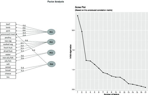
Diet is another lifestyle variable potentially associated to CRC. The UKB provides rich diet-related information collected by surveys on the day of attending the assessment center, see Section S3 in the SM for more details. Incorporating the estimated daily/weekly intakes of many different types of food will most likely induce multicollinearity. Instead, this information is processed into fewer and more meaningful variables, using exploratory factor analysis. Four factors were created, seeing that the marginal contribution in the explained variance drops substantially after the third one, see the right panel in Figure 1. Moreover, four factors offer better interpretability compared to only three, as understood by the factor loadings of the different food intakes, see the left panel in Figure 1. The factors can be roughly divided into consumption of meat, fruits and vegetables, fish, and other types of food. The fitting method used was principal axis factoring with a varimax rotation, using the psych package in R (Revelle 2022). There are other alternative methods for factor-based dimensionality reduction, see Section S4 in the SM for an analysis using one such alternative method, which eventually resulted in similar conclusions.

Fig. 1 Exploratory factor analysis based on diet variables: factor loadings and scree plot.

As for genetic risk factors, 139 SNPs that have been linked to CRC by genome-wide association studies (Thomas et al. 2020) were included, in addition to 6 genetic principal components (PC) to account for population substructure (Jeon et al. 2018). The SNPs were standardized to have mean zero and unit variance.

Usher-Smith et al. (2018) provides a comprehensive review of different CRC studies from across the world and the covariates included in them. Our analysis covers all main covariates of these models, in addition to most of the secondary ones (listed as “others” in Usher-Smith et al.). Some of the variables surveyed here do not appear in any of the studies mentioned in Usher-Smith et al. and most importantly this work also complements them with genetic information.

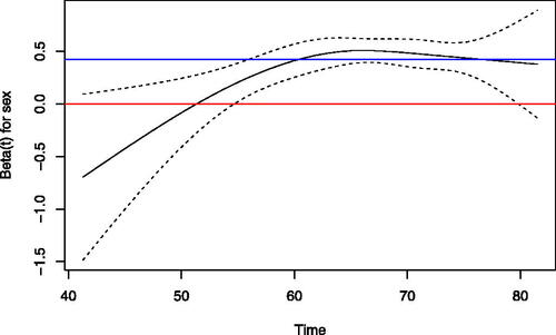
A critical assumption for the Cox model is the PH. The useful function cox.zph in the R Survival package provides Schoenfeld-residuals-based graphical and statistical tests for evaluating the necessity of time-dependent coefficients. The graphical and statistical test (p-value = 0.0006) for sex suggest a potential violation of the PH assumption, see Figure 2. Therefore, a time-dependent coefficient $\beta (t)=\{\hspace{0.17em}\ln \hspace{0.17em}(t)I(t<65)+\hspace{0.17em}\ln \hspace{0.17em}65I(t\ge 65)\}\beta$ is used, chosen based on the diagnostic graph. This coefficient implies that the hazard ratio of male to female increases over time, and plateaus around age 65. The tests for other covariates did not imply departures from the PH assumption, and are thus omitted. Although $\hspace{0.17em}\ln \hspace{0.17em}(t)$ is unbounded as t tends to 0, thus, violating the assumption in Section 3.4, it is not an actual problem since the probability of CRC before the age of 40 is practically 0 (Ouakrim et al. 2015), let alone when t tends to 0. The resultant time-dependent UKB CRC dataset comprises about 350 million rows.

Fig. 2 Diagnostic graph for the proportional-hazards assumption for sex. The red line is the 0 line and the blue line is the time-fixed coefficient. The solid curve is the spline-based estimated effect versus time, along with a confidence band.

The model includes both the environmental and the genetic covariates, totaling 180 in number. The NCC methods require generating random risk-sets for all observed event times, which is very time-consuming, and no equivalent of the reservoir-sampling algorithm exists for using NCC, so only the subsampling methods were considered with $q_n/n_e=300$. Table 1 provides the results for the environmental variables based on the full-data PL, L-R-opt, A-R-opt and the uniform subsamples, and Table S3 in the SM provides the corresponding results based on L-opt and A-opt. The genetic variables’ results can be found in Tables S4–S5 in the SM.

Table 4 Simulation results of right-censored data without delayed entry, under setting “C”, with $q_n=3n_e$: empirical SE (Emp.), estimated SEs based on the full sample (Full) and on the subsample (Sub) for each estimated regression coefficient.

	Uniform			L-opt			A-opt
	Emp.	Full	Sub	Emp.	Full	Sub	Emp.	Full	Sub
${\beta }_1$	0.4621	0.4622	0.4370	0.2874	0.2787	0.2794	0.2728	0.2666	0.2667
${\beta }_2$	0.4463	0.4493	0.4243	0.2820	0.2720	0.2727	0.2604	0.2597	0.2598
${\beta }_3$	0.0793	0.0768	0.0728	0.0457	0.0459	0.0460	0.0498	0.0488	0.0488
${\beta }_4$	0.8901	0.8852	0.8359	0.5513	0.5345	0.5357	0.5144	0.5089	0.5091
${\beta }_5$	0.0832	0.0886	0.0838	0.0548	0.0529	0.0530	0.0563	0.0556	0.0556
${\beta }_6$	0.0598	0.0607	0.0560	0.0372	0.0354	0.0354	0.0377	0.0378	0.0379
$\left|\right|.{\Vert }_F$	0.0000	0.1180	0.1951	0.0000	0.0297	0.0277	0.0000	0.0108	0.0106

NOTE: The Frobenius norm was used to calculate the distance between the empirical and estimated variance matrices.

Table 1 shows that family history, BMI, smoking, meat consumption, and the time-dependent effect of sex are all positively associated with CRC, whereas low alcohol consumption is associated with a reduced risk of CRC. These results align with existing medical knowledge, see for instance Johnson et al. (2013). Other known protective factors such as physical activity, NSAIDs, hormone use and previous screenings were not significant, neither were the sleep-related variables, male balding, vitmain D, education and non-meat consumption. Interestingly, breastfeeding was found to be significantly associated with an increased risk of CRC, supporting the findings in Yang et al. (2019). In Table 1, the p-values for all 35 environmental variables were corrected using Holm’s method (Holm 1979) and the tests were one-sided based on whether existing literature indicated the variables were protective or risk factors. The p-values are based on the L-R-opt results, and significance is considered at the 0.05 significance level. Although p-values are provided, we do not perform variable selection, and keep all the covariates in the model.

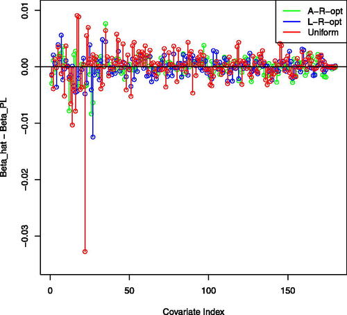
The running times for fitting the model, as required by the different methods, in hours, were 14.5, 4, 2.75, 10.5, 5.5, 0.5 for the full-data PL, L-opt, L-R-opt, A-opt, A-R-opt and uniform subsampling, respectively. For implementing the uniform subsampling when the data do not fit into the RAM we have used the reservoir algorithm. The corresponding l₂-distances with respect to the full-data PL were 0.029, 0.026, 0.020, 0.023, 0.048. The L-R-opt offers a good balance of runtime and accuracy, while being memory efficient. It substantially reduces the runtime from the full-data PL’s 14.5 hr to approximately 2.75 hr while maintaining an advantage over the uniform subsampling in terms of distance from the full-data PL. Inference on the coefficients can thus be done using the subsampled data, with a minor loss of efficiency. Figure 3 portrays the differences between the subsampling-based coefficients and their full-data PL counterparts. It demonstrates that the estimated coefficients based on the optimal subsampling methods tend to agree with the full-data PL, whereas the uniform subsampling produces larger deviations.

Fig. 3 UKB CRC data analysis: comparison between the estimated regression coefficients of each method (L-R-opt, A-R-opt, uniform). Differences with respect to the full-data PL estimator are plotted.

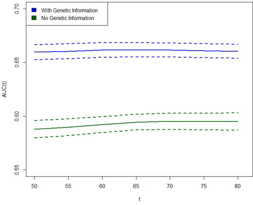
Another central objective is measuring the contribution of genetic information in CRC risk prediction, which was left out of the numerical analysis of Usher-Smith et al. To that end, the incident/dynamic time-dependent area under the receiver operating characteristics curve $\text{AUC}(t)$ of Heagerty and Zheng (2005) is adopted, which takes delayed entry into account. We have computed $\text{AUC}(t)$ with and without the SNP and genetic PC data, in increments of five years from 50 to 80, through a 10-fold cross-validation (CV) process using L-R-opt. The analysis was conducted with the risksetROC R package (Heagerty, Saha-Chaudhuri, and Saha-Chaudhuri 2012). To prevent biased CV results (Moscovich and Rosset 2022), the factor analysis of the dietary variables was conducted based on the training data of each fold, and the test dietary data were subsequently projected on the train-based factors. The $\text{AUC}(t)$ point estimates, as well as pointwise 95% confidence intervals based on 100 bootstrap repetitions are presented in Figure 4. The $\text{AUC}(t)$ estimation procedure involves postulating a Cox model for a scalar marker and exploiting its structure to cleverly calculate $\text{AUC}(t)$ efficiently. The marker in this case is the linear predictor from our time-dependent Cox model. With such a large dataset, the variability in $\text{AUC}(t)$ estimation mainly arises from the estimated coefficients of the linear predictor, offering an explanation for the constant magnitude of the standard errors over time. Evidently, the genetic information remarkably increases the predictive power of the model, indicating that even the best-performing models mentioned in Usher-Smith et al. can be further improved upon.

Fig. 4 Incident/dynamic time-dependent $\text{AUC}(t)$, for CRC diagnosis with and without genetic information, as a function of age, with 95% pointwise confidence intervals.

The full-data PL, A-opt, and L-opt methods were performed on an AWS instance x1.32xlarge, with 1952GB internal RAM, and a cost of about 22 USD per hour. The L-R-opt, A-R-opt and uniform methods were performed on a Dell XPS 15 9500, with 16GB internal RAM.

5 Simulation Study

The proposed methods were compared to the full-data PL and NCC estimators via a simulation study examining various data characteristics, including time-independent covariates under different dependency structures, with and without delayed entry, as well as time-dependent covariates affecting both censoring and event times, such that the two are conditionally independent.

To that end, 500 samples of size $n=15,000$ were generated for each scenario, using ${\mathit{\beta }}^o={(0.3,-0.5,0.1,-0.1,0.1,-0.3)}^T$, and different values for q_n. For the time-independent covariates scenario, censoring times were exponential with rate 0.2, independent of the failure times. We set ${\lambda }_0^o(t)=0.001I(t<6)+c_{{\lambda }_0}I(t\ge 6) ,$Z ${\lambda }_0^o(t)=0.001I(t<6)+c_{{\lambda }_0}I(t\ge 6) ,$ where $c_{{\lambda }_0}$, as well as the distribution of the covariates X, differed between settings “A” (no correlation, equal variances), “B” (no correlation, unequal variances) or “C” (correlated variables, mildly unequal variances), as described below.

1. $X_i\sim \text{Unif}(0,4),i=1,\dots ,6$, and are independent. $c_{{\lambda }_0}=0.05,0.015$ without and with delayed entry, respectively.

2. $X_i\sim \text{Unif}(0,u_i),u_i=1,6,2,2,1,6,i=1,\dots ,6$, respectively, and are independent. $c_{{\lambda }_0}=0.15,0.05$ without and with delayed entry, respectively.

3. $X_1,X_2,X_3$ are independently sampled from U(0, 4). $X_4=0.5X_1+0.5X_2+{\epsilon }_1,X_5=X_1+{\epsilon }_2,X_6=X_1+{\epsilon }_3$, where ${\epsilon }_1\sim N(0,0.1),{\epsilon }_2\sim N(0,1),{\epsilon }_3\sim N(1,1.5)$ and the ε’s are independent. $c_{{\lambda }_0}=0.05,0.025$ without and with delayed entry, respectively. The strongest pairwise Pearson’s correlation is about 0.75.

Delayed entry times were sampled uniformly from 0 to the third quartile of the observed times, and $n=15,000$ observations were then randomly sampled out of those satisfying T > R.

For the time-dependent covariate, we replicated the above settings without delayed entry, and added a covariate mimicking a medical test. The intervals between tests were drawn from $\text{Unif}(3,12)$, and each individual may undergo up to 4 tests. The covariate holds the cumulative number of tests at any given time, and its coefficient was set to ${\beta }_{\text{dep}}^o=0.15$, and in setting B we set $c_{{\lambda }_0}=0.05$. The censoring times are sampled similarly to the failure times, with ${\beta }^C={(0.15,-0.1,0.15,-0.1,0.15,-0.1)}^T,{\beta }_{\text{dep}}^C=0.1$, and ${\lambda }_0^C(t)=0.2I(t<6)+0.15I(t\ge 6)$. Conditionally on the covariates, the censoring and failure times are independent.

For matching controls to cases in NCC, we used the ccwc function in the Epi package (Carstensen et al. 2022). For the classic NCC (“NCC-c”), a stratified analysis was performed with coxph, whereas for Samuelsen’s improved NCC (“NCC-S”) (Samuelsen 1997), the R package MultipleNCC was used (Støer and Samuelsen 2016).

For each method, the empirical RMSE was derived, defined as $\frac{1}{500}{\sum }_{j=1}^{500}\sqrt{{\sum }_{i=1}^r{({\widehat{\beta }}_i^{(j)}-{\beta }_i^o)}^2}$ and $\frac{1}{500}{\sum }_{j=1}^{500}\sqrt{{\sum }_{i=1}^r{({\widehat{\beta }}_i^{(j)}-{\widehat{\beta }}_{\mathit{PLi}}^{(j)})}^2}$, with regards to ${\mathit{\beta }}^o$ and ${\widehat{\mathit{\beta }}}_{PL}$, respectively, where $\widehat{\mathit{\beta }}$ is the relevant estimator and the superscript (j) indicates the j’th sample. The average runtime (in seconds) and the relative RMSE (RR) are also presented, where RR is defined as the ratio of each method’s empirical RMSE to that of ${\widehat{\mathit{\beta }}}_{PL}$, with respect to the true parameter ${\mathit{\beta }}^o$.

Table 2 and Tables S6–S7 in the SM show that L-opt and A-opt tend to perform similarly with respect to RMSE and RR, with some advantage to A-opt under setting “C”. This advantage seems to shrink as the subsample size increases. Additionally, L-opt and A-opt outperform the NCC-c, NCC-S and the uniform methods under all settings. With regards to runtime, L-opt is faster than A-opt, and both are considerably faster than the full-data PL and the NCC methods, but as expected, are slower than the uniform method, which does not require computation of sampling probabilities. Thus, L-opt and A-opt offer a computational advantage over the full-data PL, without sacrificing much efficiency, while uniform sampling may incur a high efficiency loss.

Table 3 summarizes the simulation results for the time-dependent covariates setting. Note that in Approach 1 (marked with “ps”, for “pseudo”), q_n is the number of sampled rows (excluding events), while in Approach 2 (“Uniform”, “L-opt”, “A-opt”) it is the number of observations, each translating into a block of rows (see Section 3.2). As observed, Approach 1 is not inferior to Approach 2 in RMSE and RR, despite using less pseudo-observations, as those are chosen optimally, whereas Approach 2 selects whole observations, which is not optimal.

Table 3 Simulation results of right-censored data with time-dependent covariates, for scenarios A, B, C, with $q_n=3n_e$.

	${\overline{q}}_n$	Method	RMSE ${\mathit{\beta }}^o$	RR	RMSE ${\widehat{\mathit{\beta }}}_{PL}$	CR	Runtime in sec.
No delayed entry
A	1061 (54)	PL	0.128 (0.036)	1.000	0.000 (0.000)	0.957	0.199 (0.042)
		L-opt	0.142 (0.039)	1.106	0.062 (0.017)	–	0.084 (0.028)
		A-opt	0.142 (0.039)	1.106	0.061 (0.017)	–	0.091 (0.028)
		Uniform	0.260 (0.075)	2.026	0.223 (0.064)	–	0.023 (0.015)
		L-opt-ps	0.143 (0.041)	1.115	0.070 (0.019)	0.959	0.039 (0.022)
		A-opt-ps	0.145 (0.039)	1.128	0.068 (0.018)	0.960	0.041 (0.024)
B	1322 (62)	PL	0.259 (0.100)	1.000	0.000 (0.000)	0.954	0.294 (0.045)
		L-opt	0.291 (0.110)	1.125	0.138 (0.051)	–	0.113 (0.031)
		A-opt	0.288 (0.110)	1.113	0.131 (0.050)	–	0.124 (0.032)
		Uniform	0.441 (0.171)	1.705	0.358 (0.139)	–	0.033 (0.019)
		L-opt-ps	0.300 (0.115)	1.160	0.147 (0.053)	0.957	0.048 (0.019)
		A-opt-ps	0.288 (0.112)	1.114	0.139 (0.050)	0.952	0.052 (0.020)
C	1039 (56)	PL	0.569 (0.391)	1.000	0.000 (0.000)	0.947	0.196 (0.032)
		L-opt	0.647 (0.457)	1.138	0.301 (0.207)	–	0.080 (0.025)
		A-opt	0.651 (0.455)	1.144	0.302 (0.219)	–	0.087 (0.028)
		Uniform	1.201 (0.845)	2.113	0.980 (0.700)	–	0.022 (0.017)
		L-opt-ps	0.647 (0.453)	1.137	0.317 (0.223)	0.949	0.034 (0.010)
		A-opt-ps	0.637 (0.435)	1.120	0.279 (0.173)	0.952	0.037 (0.016)

NOTE: The mean ${\overline{q}}_n$ is also reported (standard errors multiplied by $\sqrt{500}$ are reported in parentheses). Using the variance formula with “Approach 2” presented additional computational difficulties, and since this approach is not superior in terms of RMSE nor in running time, the CR’s are not reported. The “ps” stands for “pseudo” (Approach 1).

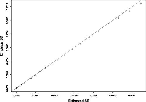
For demonstrating the finite sample performance of our proposed variance estimators, we estimated the covariance matrices of the coefficients, under setting “C”, without delayed entry, and with $q_n=3n_e$ for all 500 samples, and averaged them. Table 4 shows the empirical SD and average estimated SE of each estimated coefficient, as well as the average Frobenius distance between the empirical and estimated covariance matrices. For instance, the average Frobenius distance for L-opt is $\frac{1}{500}{\sum }_{j=1}^{500}\Vert n^{-1}{\tilde{\mathbb{V}}}_{\tilde{\mathit{\beta }}}({\mathbf{p}}^{L(j)},{\tilde{\mathit{\beta }}}_{TS}^{(j)})-\text{cov}({\tilde{\mathit{\beta }}}_{TS}){\Vert }_F ,$ where $\text{cov}({\tilde{\mathit{\beta }}}_{TS})$ is the empirical covariance matrix computed from the 500 vectors of estimated regression coefficients, and ${\tilde{\mathbb{V}}}_{\tilde{\mathit{\beta }}}$ is defined in Section 2.5 (Table 4 also shows results based on ${\mathbb{V}}_{\tilde{\mathit{\beta }}}$). For the cumulative baseline hazard function variance estimator, we calculated the empirical SD and average estimated SE in time points ranging from 0 to 10, with jumps of size 0.2. In Figure 5 the empirical SD at each time point is plotted against its estimated counterpart. Both Table 4 and Figure 5 show excellent agreement between the estimated and empirical variances. Additionally, the Wald-based 95% confidence interval coverage rate (CR) is presented for the time-fixed and the time-dependent covariates simulations under Approach 1. Since Approach 2 involves a cumbersome reconstruction of the original $\mathbf{a}(\mathit{\beta })$ vectors, the computation of the variance matrix was troublesome, and as we do not recommend this approach anyway, we skipped it. The CRs were calculated using the built-in variance estimators in the functions coxph and multipleNCC, and the estimation formula in Section 2.5. Evidently, the variance estimation and coverage rates are accurate.

Fig. 5 Simulation results of right-censored data without delayed entry, under setting “C”, for the A-opt method, with $n=15,000$ and $q_n=3n_e$: estimated SE and empirical SD for the cumulative baseline hazard function at various time points.

For validating the approximations suggested in Section 2.6 for L-R-opt and A-R-opt, we repeated settings A–C with delayed entry and $q_n=3n_e$, and the results are summarized in Table S8 in the SM. Comparing the RMSE with Table 2 reveals no efficiency loss.

The simulation study was performed on a Dell XPS 15 9500, with an Intel processor i7-10750H CPU. R code for the data analysis and reported simulations is available at Githubsite: https://github.com/nirkeret/subsampling.

6 Discussion and Future Research

We proposed fast subsampling-based estimators for the Cox model motivated by two optimality criteria under the rare-event setting. These estimators reduce computation for large datasets with minimal loss of estimation efficiency. Possible future research directions include:

• This work serves as a foundation for developing subsampling tools for other Cox-regression-based methods, such as (semi-)competing risks, frailty models, correlated data, recurrent events, and multistate models.

• Cox regression may be useful for computing sampling probabilities for other computationally-intensive methods where custom analytic derivation is challenging, such as PL-based or log-rank-based random forests (Ishwaran et al. 2008) and gradient boosting (Binder et al. 2009). When there are many covariates, a regularized Cox model is often used. Our method can generate a subsample, then a weighted regularized Cox model can be run using the glmnet package in R (Simon et al. 2011). Although expected to perform well, optimality is not guaranteed.

• Our method can be evaluated against other NCC and CC methods, on the premise of missing covariates. When some covariates are too costly to measure, one can apply our method on all fully observed data and pick a subset of observations to undergo measuring. It is interesting to find in which scenarios an improvement upon the classically used NCC and CC can be achieved.

• CRC is typically viewed as a disease mainly affecting older adults, but recent data show a rise in CRC incidence among people under 50, known as “young-onset CRC” (YOCRC) (Done and Fang 2021). It would be valuable to investigate if our model can distinguish between high and low YOCRC risk patients, based on an independent dataset with sufficient YOCRC cases.

Supplementary Materials

The supplementary materials contain the proofs for all theorems presented in this paper, and for the reservoir-sampling algorithm. Additional simulation and real-data analysis results, as well as detailed information about the UKB covariates used in the analysis are also provided.

Acknowledgments

We would like to thank Asaf Ben-Arie for programming assistance and Li Hsu for fruitful discussions. Our thanks also go to the editor, associate editor, and two referees for their constructive and interesting feedback. This research has been conducted using the UK Biobank Resource, project 56885.

Correction Statement

This article has been corrected with minor changes. These changes do not impact the academic content of the article.

Additional information

Funding

The work was supported by the Israel Science Foundation (ISF) grant number 767/21 and by a grant from the Tel-Aviv University Center for AI and Data Science (TAD).

References

- Ai, M., Yu, J., Zhang, H., and Wang, H. (2021), “Optimal Subsampling Algorithms for Big Data Regressions,” Statistica Sinica, 31, 749–772. DOI: 10.5705/ss.202018.0439.
- Binder, H., Allignol, A., Schumacher, M., and Beyersmann, J. (2009), “Boosting for High-Dimensional Time-to-Event Data with Competing Risks,” Bioinformatics, 25, 890–896. DOI: 10.1093/bioinformatics/btp088.
- Breslow, N. E. (1972), “Contribution to Discussion of Paper by D.R. Cox,” Journal of the Royal Statistical Society, Series B, 34, 216–217.
- Carstensen, B., Plummer, M., Laara, E., and Hills, M. (2022), Epi: A Package for Statistical Analysis in Epidemiology. R package version 2.47.1. https://CRAN.R-project.org/package=Epi
- Chen, C.-Y., Hu, J.-M., Shen, C.-J., Chou, Y.-C., Tian, Y.-F., Chen, Y.-C., You, S.-L., Hung, C.-F., Lin, T.-C., Hsiao, C.-W., et al. (2020), “Increased Incidence of Colorectal Cancer with Obstructive Sleep Apnea: A Nationwide Population-based Cohort Study,” Sleep Medicine, 66, 15–20. DOI: 10.1016/j.sleep.2019.02.016.
- Chen, K., and Lo, S.-H. (1999), “Case-Cohort and Case-Control Analysis with Cox’s Model,” Biometrika, 86, 755–764. DOI: 10.1093/biomet/86.4.755.
- Chun, S. K., Fortin, B. M., Fellows, R. C., Habowski, A. N., Verlande, A., Song, W. A., Mahieu, A. L., Lefebvre, A. E., Sterrenberg, J. N., Velez, L. M., et al. (2022), “Disruption of the Circadian Clock Drives APC Loss of Heterozygosity to Accelerate Colorectal Cancer,” Science Advances, 8, eabo2389. DOI: 10.1126/sciadv.abo2389.
- Cox, D. R. (1972), “Regression Models and Life-Tables,” Journal of the Royal Statistical Society, Series B, 34, 187–202. DOI: 10.1111/j.2517-6161.1972.tb00899.x.
- Davidson-Pilon, C. (2019), “lifelines: Survival Analysis in Python,” Journal of Open Source Software, 4, 1317. DOI: 10.21105/joss.01317.
- Dhillon, P., Lu, Y., Foster, D. P., and Ungar, L. (2013), “New Subsampling Algorithms for Fast Least Squares Regression,” in Advances in Neural Information Processing Systems, pp. 360–368.
- Done, J. Z., and Fang, S. H. (2021), “Young-Onset Colorectal Cancer: A Review,” World Journal of Gastrointestinal Oncology, 13, 856–866. DOI: 10.4251/wjgo.v13.i8.856.
- Garland, C., Barrett-Connor, E., Rossof, A., Shekelle, R., Criqui, M., and Paul, O. (1985), “Dietary Vitamin D and Calcium and Risk of Colorectal Cancer: A 19-year Prospective Study in Men,” The Lancet, 325, 307–309. DOI: 10.1016/s0140-6736(85)91082-7.
- Gorfine, M., Keret, N., Ben Arie, A., Zucker, D., and Hsu, L. (2021), “Marginalized Frailty-based Illness-Death Model: Application to the UK-Biobank Survival Data,” Journal of the American Statistical Association, 116, 1155–1167. DOI: 10.1080/01621459.2020.1831922.
- Heagerty, P. J., Saha-Chaudhuri, P., and Saha-Chaudhuri, M. P. (2012), Package ‘risksetroc’, Vienna, Austria: Cran R Project.
- Heagerty, P. J., and Zheng, Y. (2005), “Survival Model Predictive Accuracy and ROC Curves,” Biometrics, 61, 92–105. DOI: 10.1111/j.0006-341X.2005.030814.x.
- Holm, S. (1979), “A Simple Sequentially Rejective Multiple Test Procedure,” Scandinavian Journal of Statistics, 6, 65–70.
- Ishwaran, H., Kogalur, U. B., Blackstone, E. H., Lauer, M. S., et al. (2008), “Random Survival Forests,” The Annals of Applied Statistics, 2, 841–860. DOI: 10.1214/08-AOAS169.
- Jeon, J., Du, M., Schoen, R. E., Hoffmeister, M., Newcomb, P. A., Berndt, S. I., Caan, B., Campbell, P. T., Chan, A. T., Chang-Claude, J., et al. (2018), “Determining Risk of Colorectal Cancer and Starting Age of Screening based on Lifestyle, Environmental, and Genetic Factors,” Gastroenterology, 154, 2152–2164. DOI: 10.1053/j.gastro.2018.02.021.
- Johansson, A. L., Andersson, T. M.-L., Hsieh, C.-C., Cnattingius, S., Dickman, P. W., and Lambe, M. (2015), “Family History and Risk of Pregnancy-Associated Breast Cancer (PABC),” Breast Cancer Research and Treatment, 151, 209–217. DOI: 10.1007/s10549-015-3369-4.
- Johnson, C. M., Wei, C., Ensor, J. E., Smolenski, D. J., Amos, C. I., Levin, B., and Berry, D. A. (2013), “Meta-Analyses of Colorectal Cancer Risk Factors,” Cancer Causes & Control, 24, 1207–1222. DOI: 10.1007/s10552-013-0201-5.
- Keogh, R. H., and White, I. R. (2013), “Using Full-Cohort Data in Nested Case–Control and Case–Cohort Studies by Multiple Imputation,” Statistics in Medicine, 32, 4021–4043. DOI: 10.1002/sim.5818.
- Keum, N., Cao, Y., Lee, D., Park, S., Rosner, B., Fuchs, C., Wu, K., and Giovannucci, E. (2016), “Male Pattern Baldness and Risk of Colorectal Neoplasia,” British Journal of Cancer, 114, 110–117. DOI: 10.1038/bjc.2015.438.
- Kim, S., Cai, J., and Lu, W. (2013), “More Efficient Estimators for Case-Cohort Studies,” Biometrika, 100, 695–708. DOI: 10.1093/biomet/ast018.
- Klein, J. P., and Moeschberger, M. L. (2006), Survival Analysis: Techniques for Censored and Truncated Data, New York: Springer.
- Kolonko, M., and Wäsch, D. (2006), “Sequential Reservoir Sampling with a Nonuniform Distribution,” ACM Transactions on Mathematical Software, 32, 257–273. DOI: 10.1145/1141885.1141891.
- Kulich, M., and Lin, D. (2004), “Improving the Efficiency of Relative-Risk Estimation in Case-Cohort Studies,” Journal of the American Statistical Association, 99, 832–844. DOI: 10.1198/016214504000000584.
- Langholz, B., and Borgan, Ø. R. (1995), “Counter-Matching: A Stratified Nested Case-Control Sampling Method,” Biometrika, 82, 69–79. DOI: 10.1093/biomet/82.1.69.
- Liddell, F., McDonald, J., and Thomas, D. (1977), “Methods of Cohort Analysis: Appraisal by Application to Asbestos Mining,” Journal of the Royal Statistical Society, Series A, 140, 469–483. DOI: 10.2307/2345280.
- Lin, C.-L., Liu, T.-C., Wang, Y.-N., Chung, C.-H., and Chien, W.-C. (2019), “The Association between Sleep Disorders and the Risk of Colorectal Cancer in Patients: A Population-based Nested Case–Control Study,” In Vivo, 33, 573–579. DOI: 10.21873/invivo.11513.
- Ma, P., Mahoney, M. W., and Yu, B. (2015), “A Statistical Perspective on Algorithmic Leveraging,” The Journal of Machine Learning Research, 16, 861–911.
- McCullough, M. L., Zoltick, E. S., Weinstein, S. J., Fedirko, V., Wang, M., Cook, N. R., Eliassen, A. H., Zeleniuch-Jacquotte, A., Agnoli, C., Albanes, D., et al. (2019), “Circulating Vitamin D and Colorectal Cancer Risk: An International Pooling Project of 17 Cohorts,” Journal of the National Cancer Institute, 111, 158–169. DOI: 10.1093/jnci/djy087.
- Mittal, S., Madigan, D., Burd, R. S., and Suchard, M. A. (2014), “High-Dimensional, Massive Sample-Size Cox Proportional Hazards Regression for Survival Analysis,” Biostatistics, 15, 207–221. DOI: 10.1093/biostatistics/kxt043.
- Moscovich, A., and Rosset, S. (2022), “On the Cross-Validation Bias due to Unsupervised Preprocessing,” Journal of the Royal Statistical Society, Series B, 84, 1474–1502. DOI: 10.1111/rssb.12537.
- Ouakrim, D. A., Pizot, C., Boniol, M., Malvezzi, M., Boniol, M., Negri, E., Bota, M., Jenkins, M. A., Bleiberg, H., and Autier,P. (2015), “Trends in Colorectal Cancer Mortality in Europe: Retrospective Analysis of the WHO Mortality Database,” British Medical Journal 351.
- Prentice, R. L. (1986), “A Case-Cohort Design for Epidemiologic Cohort Studies and Disease Prevention Trials,” Biometrika, 73, 1–11. DOI: 10.1093/biomet/73.1.1.
- Pukelsheim, F. (2006), Optimal Design of Experiments, Philadelphia: SIAM.
- R Core Team (2013), R: A Language and Environment for Statistical Computing, Vienna, Austria: R Foundation for Statistical Computing.
- Raghupathi, W., and Raghupathi, V. (2014), “Big Data Analytics in Healthcare: Promise and Potential,” Health Information Science and Systems, 2, 3. DOI: 10.1186/2047-2501-2-3.
- Revelle, W. (2022), psych: Procedures for Psychological, Psychometric, and Personality Research, Evanston, IL: Northwestern University.
- Samuelsen, S. O. (1997), “A Psudolikelihood Approach to Analysis of Nested Case-Control Studies,” Biometrika, 84, 379–394. DOI: 10.1093/biomet/84.2.379.
- Simon, N., Friedman, J., Hastie, T., and Tibshirani, R. (2011), “Regularization Paths for Cox’s Proportional Hazards Model via Coordinate Descent,” Journal of Statistical Software, 39, 1–13. DOI: 10.18637/jss.v039.i05.
- Støer, N. C., and Samuelsen, S. O. (2016), “multiplencc: Inverse Probability Weighting of Nested Case-Control Data,” R Journal, 8, 5–18. DOI: 10.32614/RJ-2016-030.
- Therneau, T., Crowson, C., and Atkinson, E. (2017), “Using Time Dependent Covariates and Time Dependent Coefficients in the Cox Model,” Survival Vignettes 2, 1–25.
- Therneau, T. M. (2023), A Package for Survival Analysis in R. R package version 3.5-5. https://CRAN.R-project.org/package=survival
- Therneau, T. M., and Grambsch, P. M. (2000), “The Cox Model,” in Modeling Survival Data: Extending the Cox Model, pp. 39–77, New York: Springer.
- Therneau, T. M., Grambsch, P. M., and Fleming, T. R. (1990), “Martingale-based Residuals for Survival Models,” Biometrika, 77, 147–160. DOI: 10.1093/biomet/77.1.147.
- Thomas, M., Sakoda, L. C., Hoffmeister, M., Rosenthal, E. A., Lee, J. K., van Duijnhoven, F. J., Platz, E. A., Wu, A. H., Dampier, C. H., de la Chapelle, A., et al. (2020), “Genome-Wide Modeling of Polygenic Risk Score in Colorectal Cancer Risk,” The American Journal of Human Genetics, 107, 432–444. DOI: 10.1016/j.ajhg.2020.07.006.
- Usher-Smith, J., Harshfield, A., Saunders, C., Sharp, S., Emery, J., Walter, F., Muir, K., and Griffin, S. (2018), “External Validation of Risk Prediction Models for Incident Colorectal Cancer Using UK Biobank,” British Journal of Cancer, 118, 750–759. DOI: 10.1038/bjc.2017.463.
- Wang, H., and Ma, Y. (2021), “Optimal Subsampling for Quantile Regression in Big Data,” Biometrika, 108, 99–112. DOI: 10.1093/biomet/asaa043.
- Wang, H., Zhu, R., and Ma, P. (2018), “Optimal Subsampling for Large Sample Logistic Regression,” Journal of the American Statistical Association, 113, 829–844. DOI: 10.1080/01621459.2017.1292914.
- Wang, Y., Hong, C., Palmer, N., Di, Q., Schwartz, J., Kohane, I., and Cai, T. (2021), “A Fast Divide-and-Conquer Sparse Cox Regression,” Biostatistics, 22, 381–401. DOI: 10.1093/biostatistics/kxz036.
- Yang, T. O., Cairns, B. J., Green, J., Reeves, G. K., Floud, S., Bradbury, K. E., and Beral, V. (2019), “Adult Cancer Risk in Women who were Breastfed as Infants: Large UK Prospective Study,” European Journal of Epidemiology, 34, 863–870. DOI: 10.1007/s10654-019-00528-z.
- Yu, J., Wang, H., Ai, M., and Zhang, H. (2022), “Optimal Distributed Subsampling for Maximum Quasi-Likelihood Estimators with Massive Data,” Journal of the American Statistical Association, 117, 265–276. DOI: 10.1080/01621459.2020.1773832.
- Zhang, H., Zuo, L., Wang, H., and Sun, L. (2022), “Approximating Partial Likelihood Estimators via Optimal Subsampling,” arXiv preprint arXiv:2210.04581. DOI: 10.1080/10618600.2023.2216261.
- Zhang, X., Giovannucci, E. L., Wu, K., Gao, X., Hu, F., Ogino, S., Schernhammer, E. S., Fuchs, C. S., Redline, S., Willett, W. C., et al. (2013), “Associations of Self-reported Sleep Duration and Snoring with Colorectal Cancer Risk in Men and Women,” Sleep, 36, 681–688. DOI: 10.5665/sleep.2626.
- Zheng, Y., Brown, M., Lok, A., and Cai, T. (2017), “Improving Efficiency in Biomarker Incremental Value Evaluation Under Two-Phase Designs,” The Annals of Applied Statistics, 11, 638–654. DOI: 10.1214/16-AOAS997.
- Zuo, L., Zhang, H., Wang, H., and Liu, L. (2021), “Sampling-based Estimation for Massive Survival Data with Additive Hazards Model,” Statistics in Medicine, 40, 441–450. DOI: 10.1002/sim.8783.