Accommodating Time-Varying Heterogeneity in Risk Estimation under the Cox Model: A Transfer Learning Approach

Abstract

Transfer learning has attracted increasing attention in recent years for adaptively borrowing information across different data cohorts in various settings. Cancer registries have been widely used in clinical research because of their easy accessibility and large sample size. Our method is motivated by the question of how to use cancer registry data as a complement to improve the estimation precision of individual risks of death for inflammatory breast cancer (IBC) patients at The University of Texas MD Anderson Cancer Center. When transferring information for risk estimation based on the cancer registries (i.e., source cohort) to a single cancer center (i.e., target cohort), time-varying population heterogeneity needs to be appropriately acknowledged. However, there is no literature on how to adaptively transfer knowledge on risk estimation with time-to-event data from the source cohort to the target cohort while adjusting for time-varying differences in event risks between the two sources. Our goal is to address this statistical challenge by developing a transfer learning approach under the Cox proportional hazards model. To allow data-adaptive levels of information borrowing, we impose Lasso penalties on the discrepancies in regression coefficients and baseline hazard functions between the two cohorts, which are jointly solved in the proposed transfer learning algorithm. As shown in the extensive simulation studies, the proposed method yields more precise individualized risk estimation than using the target cohort alone. Meanwhile, our method demonstrates satisfactory robustness against cohort differences compared with the method that directly combines the target and source data in the Cox model. We develop a more accurate risk estimation model for the MD Anderson IBC cohort given various treatment and baseline covariates, while adaptively borrowing information from the National Cancer Database to improve risk assessment. Supplementary materials for this article are available online.

KEYWORDS:

• Cox proportional hazards model
• Inflammatory breast cancer
• National Cancer Database
• Risk assessment
• Transfer learning

1 Introduction

Estimating the risk of a failure event is an important topic in clinical research for chronic diseases such as cardiovascular disease and cancer (Jiao et al. 2018; Kumar et al. 2020). If the population of interest comes from a single institution or a clinical trial, however, the limited sample size may prevent accurate individualized risk assessment, especially for rare diseases. Here, we consider a rare but aggressive type of cancer called inflammatory breast cancer (IBC) (Jaiyesimi, Buzdar, and Hortobagyi 1992). Although IBC constitutes only 1% to 6% of all breast cancer patients in the United States, the diagnosed patients have a worse prognosis with five-year survival of around 34% to 47% (Masuda et al. 2014). IBC patients seen at the Morgan Welch Inflammatory Breast Cancer Research Program and Clinic at The University of Texas MD Anderson (MDA) Cancer Center are the target population of this study. Although MD Anderson Cancer Center is a leading cancer care institute, the performance of risk assessment using the data of the MDA cohort alone is far from satisfactory due to the rarity of the disease. Large population-based registry data sources, including the Surveillance, Epidemiology and End Results (SEER) and the National Cancer Database (NCDB), have been increasingly used as complement data cohorts because of their easy accessibility and large sample size (Carvalho et al. 2005; Bilimoria et al. 2008).

Combining information from outside registry data (i.e., the source cohort) in the analysis of the target cohort (e.g., the MDA IBC cohort in the motivating example) has been a promising solution to the small sample size problem in risk estimation. NCDB data were obtained as our source cohort in the motivating example. Cancer registries have been used as auxiliary information to improve statistical inference in recent literature (Chatterjee et al. 2016; Antonelli, Zigler, and Dominici 2017; Chen et al. 2021). Specifically, Chatterjee et al. (2016) and Huang, Qin, and Tsai (2016) developed likelihood-based frameworks to borrow information from external data sources in regression models. Most of these methods rely on an essential assumption, that is, the two study populations are comparable (Chatterjee et al. 2016; Li et al. 2022). This assumption is often violated in practice. It is well noted that there is substantial referral bias in the MDA population compared to general patients from cancer registries, that is, the MDA patients may have more complicated conditions or delayed diagnosis (Carlé et al. 2013). In our motivating example, the MDA-IBC cohort has a worse prognosis compared to the IBC patients of the NCDB cohort due to referral bias, suggesting substantial heterogeneity between the cohorts. An essential question here is how and to what extent we can learn from using cancer registry data in the risk estimation. Both Liu et al. (2014) and Huang, Qin, and Tsai (2016) modified the Cox model by relaxing the cumulative hazard function in the target population and multiplying a constant factor. Still, their methods could not address the potential differences in the baseline hazards of the two populations. A recent work by Chen et al. (2021) developed an adaptive estimation procedure, which allows the source population to be incomparable with the target population. They used summary statistics to adjust the level of information borrowed from external sources. This is a promising approach, but it is also restricted in that only the summary level survival data, such as 10-year survival rate, can be borrowed from the external data.

Recently, a few transfer-learning-based statistical methods have been proposed to adaptively borrow information from the source population under different analysis frameworks. The advantage of these transfer-learning approaches is that, even when the external population is dramatically different from the target cohort, termed “negative transfer,” these methods can still provide reasonable estimations because the level of information borrowing was adaptively determined by the data similarities. The considered scenarios include transfer learning in Gaussian graphical models (Li, Cai, and Li 2022), nonparametric classification (Cai and Wei 2021), high-dimensional linear regression (Li, Cai, and Li 2020), generalized linear models (GLM) (Tian and Feng 2022), and federated learning with GLM (Li, Cai, and Duan 2021). However, none of these methods can be applied to the analysis of time-to-event outcomes, as considered in the motivating problem. Cox models are widely used for assessing risk with time-to-event data due to their easy interpretation and model flexibility (Cox 1972). There are a number of additional statistical challenges in transferring the knowledge from the source to the target cohort in lifetime analysis under the Cox models. First, compared to the transfer learning in the regression setting in which models borrow information for the coefficients only, Cox models would be represented by different baseline hazard functions when the source and target cohorts have time-varying risk shifts. Additionally, the coefficients of baseline covariates and baseline hazards in the Cox models could have different but dependent levels of information sharing, and thus they should be controlled simultaneously. Second, the baseline cumulative hazards function is routinely estimated semi-parametrically in the framework of Cox models. The jump points of its estimation are decided by the event times in the observed data. As a result, the target and source populations can have distinct sets of breakpoints for the baseline hazard estimations, which makes information borrowing more challenging. Third and finally, individual-level data may not always be available for the source population due to privacy and logistical concerns (Platt and Kardia 2015). The desired method should be able to allow both scenarios, that is, using individual-level data or incorporating summary statistics obtained from the source population without the need to share individual-level data.

In this article, we address all the aforementioned challenges in transfer learning for time-to-event data under the Cox models. The proposed method overcomes the difficulty of sharing information with different sets of event times in the two cohorts. We allow different levels of information borrowing in the regression coefficients and baseline hazards through tuning parameters, and the resultant estimates are obtained in a unified framework simultaneously. As a result, the proposed method has great flexibility in that both covariate distributions and the associated coefficients, as well as baseline hazards are all allowed to be different between the two cohorts. As shown in our extensive simulation studies, the proposed method demonstrates satisfactory robustness, accuracy, and efficiency gained even when the source and target cohorts are heterogeneous in varying patterns and degrees. The applications to the MDA IBC cohort with NCDB data as a complement cohort also suggest improved precision of risk estimation compared with a regular Cox model with the MDA cohort alone. We present the notation, model, and algorithm in Section 2. The results from the simulation studies are present in Section 3 to evaluate the empirical performance. In Section 4, we present the data analysis results for the motivating example with IBC cohorts and interpret the results. We provide concluding remarks and discussions in Section 5.

2 Method

2.1 Notation and Model

Denote the outcome, the time from an initial event to an event of interest, by T. Let the covariates of interest be the p-dimensional vector $\mathit{X}$. Given $\mathit{X}=\mathit{x}$, define the conditional density function and conditional survival function of T as $f(T|\mathit{x})$ and $S(T|\mathit{x})$. We denote the censoring time by C and the occurrence of the interested events (e.g., time to death) by $\delta =I(T\le C)$. In the context of transfer learning, we have two sets of cohorts: a target cohort and a source cohort. The target cohort consists of N independent samples, $\{(Y_i,{\delta }_i,{\mathit{X}}_i),i=1,\dots ,N\}$, where $Y_i=\mathit{textrmmin}\{T_i,C_i\},{\delta }_i=I(T_i\le C_i)$. Let the number of unique event time points in the target cohort be n₀.

In the target cohort, the Cox model assumes the covariate specific hazard function follows $$h(t|{\mathit{X}}_i)=h_0(t)\mathit{textrmexp}({\mathit{X}}_i^T\mathit{\beta }), i=1,\dots ,N.$$Here, $\mathit{\beta }$ is the p-dimensional vector of regression coefficients and $h_0(·)$ is an unspecified baseline hazard function.

For the source cohort, we consider two scenarios when the individual-level data are or are not available. When the individual-level data are available, the source cohort is represented by N ${}^s$ independent observations, $\{(Y_i^s,{\delta }_i^s,{\mathit{X}}_i^s),i=1,\dots ,N^s\}$. The number of unique event time points is $n_0^s$. The corresponding Cox model for the source population also has the proportional hazards assumption, $$h^s(t|{\mathit{X}}_i^s)=h_0^s(t)\mathit{textrmexp}\{{({\mathit{X}}_i^s)}^T{\mathit{\beta }}^s\}, i=1,\dots ,N^s,$$where $h_0^s(·)$ is an unspecified baseline hazard function. The cumulative baseline hazard function is denoted by $H_0^s(t)={\int }_0^t{h}_0^s(u)du$. If the individual-level data cannot be shared due to privacy and logistical concerns, the proposed method still works given the estimators of coefficients ${\widehat{\mathit{\beta }}}^s$ and baseline cumulative hazards ${\widehat{H}}_0^s(·)$, which can be transferred by the source cohort site.

In addition to the proportional hazards assumption, we assume that the same set of covariates are available in both cohorts. However, the distributions of the covariates are allowed to be different in the two cohorts, which is termed as a “covariate shift” (Sugiyama, Krauledat, and Müller 2007; Jeong and Namkoong 2020). Note that we do not need to assume the two cohorts are comparable, that is, the regression coefficient ${\mathit{\beta }}^s$ and baseline cumulative hazards $H_0^s(·)$ in the source cohort can be different from $\mathit{\beta }$ and $H_0(·)$ in the target cohort, as well as the covariate distribution.

2.2 Transfer Learning Algorithm

With both the target and the source cohorts, a naïve approach to obtaining a more accurate risk assessment model is to combine data from the two cohorts and apply a Cox model. However, it is possible that the source cohort is different from the target cohort, which would lead to biased estimates (or risk estimation) of the target cohort. Even if the differences of the coefficients and baseline hazards in the two cohorts are small, the estimation bias by combining the two datasets can still be substantial when the sample size of the source cohort is much larger than that of the target cohort. To facilitate borrowing information from the source cohort, which may or may not be similar to the target cohort, our solution is to propose a transfer learning algorithm, called Trans-Cox, for improving the efficiency and accuracy of risk estimation for the target cohort.

When the individual-level data from the source cohort is available, we fit a Cox model using the source cohort only. Denote the ordered observed unique failure times in the target dataset by $\{{\tilde{y}}_1,\dots ,{\tilde{y}}_{n_0}\}$ and in the source dataset by $\{{\tilde{y}}_1^s,\dots ,{\tilde{y}}_{n_0^s}^s\}$. The log-likelihood for modeling the source cohort is (1) $$\begin{array}{c}l({\mathit{Y}}^s,{\mathit{X}}^s,{\mathit{\delta }}^s;H^s,{\mathit{\beta }}^s)=\sum _{i=1}^{N^s}{\delta }_i^s[{({\mathit{X}}_i^s)}^T{\mathit{\beta }}^s+\hspace{0.17em}\log \hspace{0.17em}\{h_i^s\left\}\right]\\ \hspace{1em}-\sum _{i=1}^{N^s}{H}_0^s(Y_i^s)\hspace{0.17em}\exp \hspace{0.17em}\left\{{({\mathit{X}}_i^s)}^T{\mathit{\beta }}^s\right\},\end{array}$$(1) where $h_i^s=\mathrm{d}{H}_0^s(Y_i^s)$. After inserting the Breslow estimator of the baseline hazard function (Breslow 1972), $${\widehat{h}}_j^s({\mathit{\beta }}^s)={(\sum _{i\in \mathcal{R}({\tilde{y}}_j^s)}\hspace{0.17em}\exp \hspace{0.17em}\{{({\mathit{X}}_i^s)}^T{\mathit{\beta }}^s\})}^{-1},$$ the baseline cumulative hazard function is estimated by ${\widehat{H}}_0^s(t)=\sum _{j=1}^{n_0^s}{\widehat{h}}_j^{s}I({\tilde{y}}_j^s\le t)$, where $\mathcal{R}(t)=\{j:{\tilde{y}}_j^s\ge t\}$ is the risk set at t. We obtain the partial likelihood, (2) $$l({\mathit{\beta }}^s)=\sum _{i=1}^{N^s}{\delta }_i^s{(X_i^s)}^T{\mathit{\beta }}^s-\sum _{i=1}^{N^s}{\delta }_i^s\hspace{0.17em}\log \hspace{0.17em}(\sum _{j\in \mathcal{R}(Y_i^s)}\hspace{0.17em}\exp \hspace{0.17em}\{{({\mathit{X}}_j^s)}^T{\mathit{\beta }}^s\}).$$(2)

The coefficients in the source cohort ${\widehat{\mathit{\beta }}}^s$ can be estimated by maximizing (2), and the cumulative baseline hazards can be estimated from the Breslow estimator (3) $${\widehat{H}}_0^s(t)=\sum _{i=1}^{N^s}\frac{I(Y_i^s\le t){\delta }_i^s}{\sum _{j\in \mathcal{R}(Y_i^s)}\hspace{0.17em}\exp \hspace{0.17em}\left\{{({\mathit{X}}_j^s)}^T{\widehat{\mathit{\beta }}}^s\right\}}.$$(3)

In reality, sharing individual-level data can be challenging across multiple sites due to different data sharing policies for privacy, feasibility, and other concerns (Karr et al. 2007; Toh 2020). Instead of sharing the individual-level data, a more practical approach is to share the summary-level statistics from external sites and draw conclusions using meta-analysis or distributed analysis (Lin and Zeng 2010; Li et al. 2018). Our proposed method shares the same principle as the distributed analysis. When individual data are not available, our proposed method takes summary statistics in the form of estimated coefficients ${\widehat{\mathit{\beta }}}^s$ and cumulative baseline hazards ${\widehat{H}}_0^s(·)$ from the source cohort to achieve the same purpose. The whole analysis procedure (described below) demonstrates how the same outcomes are obtained with individual-level data or with summary statistics only.

Starting from the estimated coefficients ${\widehat{\mathit{\beta }}}^s$ and the cumulative baseline hazard function ${\widehat{H}}_0^s(·)$, we first obtain the “source” version of hazard estimations at the event times of the target cohort by creating a reference hazard estimation. We define the reference hazards $\Delta {\widehat{H}}_0^s(t)$ at $t={\tilde{y}}_i$ by the difference of the baseline cumulative hazards function from the source dataset at the neighboring two consecutive time points of the target cohort, that is, (4) $$\Delta {\widehat{H}}_0^s({\tilde{y}}_i)={\widehat{H}}_0^s({\tilde{y}}_i)-{\widehat{H}}_0^s({\tilde{y}}_{i-1}), i=1,\dots ,n_0.$$(4)

When inferring the risk estimation through the Cox model to the target cohort, we allow the two to be different by assuming that (5) $$\mathit{\beta }={\widehat{\mathit{\beta }}}^s+\mathit{\eta } \mathit{textrmand} \mathrm{d}{H}_0({\tilde{y}}_j)=\Delta {\widehat{H}}_0^s({\tilde{y}}_j)+{\xi }_j, j=1,\dots ,n_0.$$(5)

The two sets of parameters, $\mathit{\eta }$ and $\mathit{\xi }=({\xi }_1,\dots ,{\xi }_{n_0})$, are to quantify potential discrepancies in the covariate effects and the time-varying baseline hazard. When the two resources are comparable in terms of risk models, the two sets of parameters degenerate to zero, that is, $\mathit{\eta }=\mathit{\xi }=\mathit{0}$. Otherwise, there exists at least one nonzero component of the two vectors. Under this scenario, directly transferring the estimated Cox model from the source cohort to target cohort or combining the two cohorts for joint estimation would result in biased risk estimation. Our strategy is to estimate and identify a nonzero subset of these parameters adaptively for this scenario using information from the two resources.

Inspired by the penalized likelihood for variable selection in regression analysis, we add an L-1 penalty to the changing terms to control the sparsity and let the data drive the magnitude of source cohort information borrowing. With the formulation (5), the objective function to be minimized is (6) $$\begin{array}{c}O(\mathit{\eta },\mathit{\xi },{\lambda }_{\eta },{\lambda }_{\xi })\\ \hspace{1em}=-\sum _{i=1}^N{\delta }_i[{\mathit{x}}_i^T({\widehat{\mathit{\beta }}}^s+\mathit{\eta })+\hspace{0.17em}\log \hspace{0.17em}\{\Delta {\widehat{H}}_0^s(y_i)+{\xi }_i\left\}\right]\\ \hspace{1em}\hspace{1em}+\sum _{i=1}^N\left[\sum _{j=1}^{n_0}\{\Delta {\widehat{H}}_0^s({\tilde{y}}_j)+{\xi }_j\}I({\tilde{y}}_j\le y_i)\right]\mathit{textrmexp}\{{\mathit{x}}_i^T({\widehat{\mathit{\beta }}}^s+\mathit{\eta })\}\\ \hspace{1em}\hspace{1em}+{\lambda }_{\eta }\left|\right|\mathit{\eta }|{|}_1+{\lambda }_{\xi }|\left|\mathit{\xi }\right|{|}_1,\end{array}$$(6) where ${\lambda }_{\eta }$ and ${\lambda }_{\xi }$ are tuning parameters controlling the sparsity. The optimal values of ${\lambda }_{\eta }$ and ${\lambda }_{\xi }$ can be selected using the Bayesian Information Criterion (BIC) (Neath and Cavanaugh 2012) with grid search. Our proposed Trans-Cox algorithm is formally presented in Algorithm 1.

Algorithm 1:

Trans-Cox algorithm

Data: Individual-level data from target cohort $(\mathit{X},\mathit{Y},\mathit{\delta })$; Individual-level data $({\mathit{X}}^s,{\mathit{Y}}^s,{\mathit{\delta }}^s)$ or summary statistics {${\widehat{\mathit{\beta }}}^s,{\widehat{H}}_0^s$} from the source cohort.

Result: $\widehat{\mathit{\beta }},{\widehat{H}}_0$ Step 1. Obtain ${\widehat{\mathit{\beta }}}^s$ and ${\widehat{H}}_0^s$ from source cohort.if $({\mathit{X}}^s,{\mathit{Y}}^s,{\mathit{\delta }}^s)$ available then

Estimate coefficients ${\widehat{\mathit{\beta }}}^s$ by maximizing the partial log-likelihood defined in (2);

Estimate cumulative baseline hazards ${\widehat{H}}_0^s$ by (3).else

Take ${\widehat{\mathit{\beta }}}^s$ and ${\widehat{H}}_0^s$ as inputs.end

Step 2. Estimate reference hazards at the unique event time points of the target cohort by (4).

Step 3. Identify values for tuning parameters ${\lambda }_{\eta },{\lambda }_{\xi }$, τ_lr, and τ_sp using BIC. τ_lr and τ_sp are defined in Section 2.3.

Step 4. Estimate $(\widehat{\mathit{\eta }},\widehat{\mathit{\xi }})$ by minimizing the objective function (6). The estimated coefficients and baseline hazards of the target cohort are $$\widehat{\mathit{\beta }}={\widehat{\mathit{\beta }}}^s+\widehat{\mathit{\eta }} \mathit{textrmand} \mathrm{d}{\widehat{H}}_0(\tilde{\mathit{y}})=\Delta {\widehat{H}}_0^s(\tilde{\mathit{y}})+\widehat{\mathit{\xi }}.$$

The cumulative baseline hazards function is ${\widehat{H}}_0(t)={\sum }_{i=1}^{n_0}\mathrm{d}{\widehat{H}}_0({\tilde{y}}_i)I({\tilde{y}}_i\le t)$

2.3 Remark on Optimization

Solving the objective function (6) is a challenging nonlinear optimization problem. We implement the minimization using R 4.0.3 by invoking the TensorFlow (Dillon et al. 2017) solver from Python. This core optimization step is solved by the “tfp.math.minimize” function from TensorFlow probability (Dürr, Sick, and Murina 2020). After the required Python environment has been installed, users can use all the Trans-Cox functions we coded in R without additional coding in Python. To achieve optimal numerical performance, the TensorFlow functions need the inputs of two additional tuning parameters: learning rate τ_lr and number of steps τ_sp. For any given target data, we first select the combination of τ_lr and τ_sp with the smallest BIC values by fixing the other two tuning parameters ${\lambda }_{\eta }$ and ${\lambda }_{\xi }$ as 0.1. Then we fix τ_lr and τ_sp as the selected values, and we select the optimal set of ${\lambda }_{\eta }$ and ${\lambda }_{\xi }$ with BIC. Our method has been implemented in a user-friendly R package Trans-Cox with a detailed usage manual, and it is publicly available at https://github.com/ziyili20/TransCox.

3 Simulation

We conduct simulation studies to evaluate the finite sample performance of the proposed Trans-Cox algorithm. We also compare the performance of the Trans-Cox results with those of the standard Cox regression models using the target cohort only, the naïve combination of target and source cohorts, or the stratified Cox model.

3.1 Simulation Set-Ups

Without loss of generality, we assume that individual data of both cohorts are available. For both cohorts, we consider five covariates $\mathit{X}={(X_1,X_2,X_3,X_4,X_5)}^T$. Of these, X₁, X₄ and X₅ are continuous covariates following a uniform distribution ranging from 0 to 1 and X₂ is a binary variable from a Bernoulli distribution with p = 0.5. Taking into account the potentially different distributions of covariates between the target and source cohorts, we assume that X₃ follows a standard uniform distribution in the target cohort, whereas it follows a $\mathit{textrmBeta}(1,2)$ distribution in the source cohort. We generate the covariate-specific survival times from a Weibull distribution with a hazard function $h(t|\mathit{X})=\kappa t·\mathit{textrmexp}({\mathit{X}}^T\mathit{\beta })$, where $\mathit{\beta }={(-0.5,0.5,0.2,0.1,0.1)}^T$ and κ = 2 for the target cohort. To mimic real-world scenarios in practice, we consider a total of four simulation settings for the source cohort. The source samples in the first setting are generated using the exact parameters as those of the target cohort. The source samples in the second setting are generated by changing β₂ from 0.5 to 0.2, which enables us to evaluate the performance of Trans-Cox when the covariate X₂ has different effects on the survival time between two cohorts. In the third setting, the two cohorts share the same regression coefficients but have different time-varying hazard functions, which reflects a different baseline risk for the outcome of interest (e.g., overall worse or improved survival over time for the patients). Specifically, we set the baseline hazard function of the source cohort as 3t (i.e., κ = 3), indicating there is a time-varying risk shift between two resources. The last setting allows both the regression coefficients and baseline hazard functions to be different, indicating less shared information between the two cohorts (${\beta }_2=0.2$, κ = 3).

It is worth noting that the cumulative baseline hazards in Settings 3 and 4 exhibit significant differences between the two cohorts, as shown in Figure S1, indicating that the amount of shared knowledge between the cohorts regarding baseline hazards is limited. For this simulation study, the sample size is fixed at N = 250 and N_s = 6400 to best mimic the observation amount in the real data application. In our evaluation, we compare the proposed Trans-Cox algorithm with two direct applications of Cox regressions with the target cohort only (i.e., Cox-Tonly) and with the combined cohort (i.e., Cox-Both), as well as stratified Cox with the combined cohort (i.e., Cox-Str). We further evaluate the bootstrap-based variance estimation using simulation study. The tuning parameters τ_lr, τ_sp, ${\lambda }_{\eta }$, and ${\lambda }_{\xi }$ are selected using BIC (Burnham and Anderson 2004).

3.2 Simulation Results

Figure 1 summarizes the simulation results of the first three estimated regression coefficients (Panel A). To save space, the estimates for the fourth and fifth coefficients are not included as they have similar bias levels to the first one as the three covariates share the same uniform distribution in the two cohorts. We present the estimated biases using the four methods under four simulation settings. Note that the results from Cox-Tonly remain the same across the four settings as the differences across the settings only occur in the source cohort. For regression coefficients, the Trans-Cox results have smaller variations than Cox-Tonly while maintaining a similar level of biases. For example, the mean biases($\times {10}^3$) for estimating β₁ by Trans-Cox models are 14.4, 13.3, 3.3, and 54.2 in the four settings, respectively, while the mean bias($\times {10}^3$) of the Cox model using the target cohort only is -27.1. The corresponding standard deviations (SD $\times {10}^3$) of β₁ by Trans-Cox (169.5, 170.3, 50.4, and 93.6, respectively) are about half the SD by Cox-Tonly for β₁ (265.6). It is expected that Cox-Both tends to provide even smaller estimated variances and biases if the two cohorts have the same risk models. However, the biases by Cox-Both can be substantially larger when the two cohorts are heterogeneous in terms of regression coefficients or baseline hazards. In Settings 2 and 4, the estimation biases($\times {10}^3$) of β₂ by Cox-Both (–291.4 and –296.8) are four to six times the biases by Trans-Cox (–50.2 and –82.3). Stratified Cox presents similarly poor results as Cox-Both when the true coefficients are different in the two cohorts (Settings 2 and 4). The gray dotted lines in Figure 1(A) mark the place where the estimation biases are zero. It is clear that Cox-Both and Cox-Str have more biased boxes in Settings 2 and 4 (dark green and dark orange boxes), while the boxes representing Trans-Cox (red) and Cox-Tonly (blue) have similarly good performance (closer to the gray line) in all settings. It is also worth noting that different covariate coefficients in the two cohorts have a minimum impact on the estimations by Trans-Cox and Cox-Str, but affect the estimation by Cox-Both in Settings 3 and 4.

Fig. 1 Estimation biases for coefficients β₁, β₂, and β₃ (Panel A), as well as cumulative baseline hazards at times 0.6 and 1.2 (Panel B) over 100 Monte Carlo simulations. $H_1={\widehat{H}}_0(0.6)$ and $H_2={\widehat{H}}_0(1.2)$. The dotted gray line shows the place where bias equals zero.

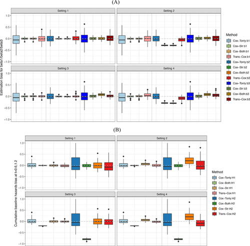
We report the biases of the cumulative baseline hazard estimators at two time points, $H_1=H_0(t=0.6)$ and $H_2=H_0(t=1.2)$, by the four methods in Figure 1(B). An interesting observation is that there is no major negative impact on the baseline hazards estimation when the regression coefficients differ between the two cohorts except for the stratified Cox model (Setting 2). Aside from this, we observe similar patterns for the estimator of cumulative baseline hazards as seen for regression coefficients. The biases from Trans-Cox and Cox-Tonly are comparable, while the SDs by Trans-Cox are about half of those by Cox-Tonly. The biases by Cox-Both are smaller and the SDs are about one fifth of those by Cox-Tonly. However, in Settings 3 and 4, when the risk models have different baseline hazards in the two cohorts, the biases of the cumulative baseline hazards at the two time points can be as high as 10 times the biases by Trans-Cox or Cox-Tonly. In Figure 1(B), the results by Cox-Both (green boxes) show striking distances from the zero-bias line compared to the other two methods (red and blue boxes).

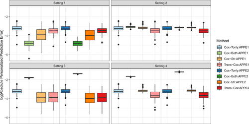
In Figure 2, we compare the personalized prediction accuracy using the absolute error between the individual predicted probability and the true survival probability (APPE1 and APPE2) across all subjects at time 0.6 and 1.2. Cox-Both exhibits the smallest absolute prediction error in the first setting, outperforming the other three methods. However, as expected, Cox-Both demonstrates substantially larger errors in Settings 3 and 4. Overall, Trans-Cox achieves the smallest errors in Settings 2, 3, and 4, and it is robust to cohort heterogeneity compared to the other methods. The corresponding numerical values for the mean biases and standard deviations are presented in Table S1 along with the restricted mean survival times (RMSTs) and mean squared errors (MSEs). RMST measures the average survival up to the specific time points (t = 0.6 and 1.2 in Table S1) for a fixed covariate combination ($\mathit{X}=(0.5,1,0.1,0.5,0.5)$). MSE quantifies the mean squared estimation error of the baseline cumulative function at times 0.6 and 1.2. Trans-Cox generally has the smallest MSE for estimating the regression coefficients, as well as the smallest RMST and the smallest absolute personalized predictive error (APPE) compared to the other three methods when the two cohorts differ.

Fig. 2 Boxplots for absolute personalized prediction error of Trans-Cox and other existing methods in different simulation settings at time 0.6 (APPE1) and 1.2 (APPE2). The results are summarized over 100 Monte Carlo datasets.

We perform additional simulation settings to further evaluate the impact of distribution shift, which is often observed in age-related data analysis. For this scenario, X₃ follows normal distribution with mean 0 and variance 1 in the target cohort but mean 0.5 in the source cohort. Our findings, presented in Figure S2, demonstrate similar trends. Trans-Cox shows smaller estimation variance with comparable bias levels to the Cox regression with target data only. We provide the exact estimation biases with standard deviations for the regression coefficients β₁, β₂, and β₃, cumulative baseline hazards at times 0.6 and 1.2, RMST, and MSE for the corresponding scenarios in Table S2.

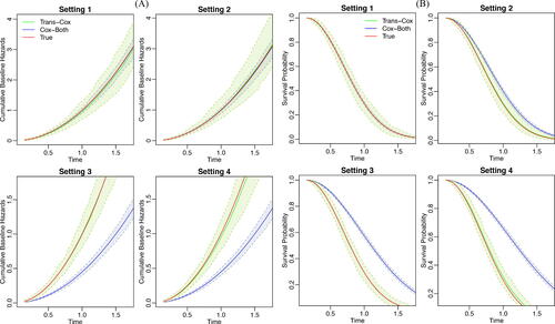
Moreover, we visualize the estimated cumulative baseline hazard curves and the survival curves for our proposed method and the Cox regression using the combined cohort in Figure 3. The shaded areas represent the 95% empirical confidence intervals, which are obtained by taking the 0.025 and 0.975 percentiles from the repeated experiments. The survival curve is evaluated at the fixed covariate combination ($\mathit{X}=(0.5,1,0.1,0.5,0.5)$). We do not include Cox-Tonly and Cox-Str on these figures. This is because the lines almost overlap with the Trans-Cox inference while having consistently wider confidence intervals. We show that the cumulative baseline hazards and the survival curves estimated by the Trans-Cox method are close to the true curves in all four settings. Cox-Both leads to substantial biases in Settings 3 and 4 where the true baseline cumulative hazards are different in the two cohorts. Similar observations can be found in the setting with a normal distribution shift in the two cohorts (Figure S3).

Fig. 3 The estimated cumulative baseline hazard (Panel A) and the survival curves (Panel B) for Trans-Cox (green) and Cox-Both (blue) in comparison to the true curves (red) over 100 Monte Carlo experiments. For survival curves, the covariates are fixed at $\mathit{X}=(0.5,1,0.1,0.5,0.5)$.

For the bootstrap-based variance estimation in Trans-Cox, Table S3 shows reasonable standard error estimations and coverage probability. As expected, the coverage probabilities generally are closer to the nominal value in the settings when the coefficients are the same in the two cohorts (Settings 1 and 3). Larger sample sizes do not offer a substantial improvement in the performance, indicating the need to tailor the standard bootstrapping method for more accurate inference in future research.

Lastly, we present the estimation sparsity of the parameters ($\mathit{\eta },\mathit{\xi }$) in Figure S5 and evaluate the computational cost of Trans-Cox in various settings in Figure S9. As expected, there are more zero or close-to-zero estimations in $\mathit{\xi }$ than $\mathit{\eta }$ due to the high dimension of the event time points in the target cohort. Our implementation offers superior computational performance, with the functions implemented in R and a core solver invoked from Python. A run with 200 patients in the target cohort on average takes around 0.6 sec, and with 400 patients it takes about 1 sec (Figure S9). The size of the source population has a minimum impact on the total computational time. The fast speed makes it feasible to construct a bootstrap-based variance estimation. For example, it takes about 21 min to complete 1000 bootstrap iterations in the IBC application (target cohort: 251 patients; source cohort: 6420 patients) of Section 4.

4 Data Application

The Morgan Welch Inflammatory Breast Cancer Clinic at MD Anderson Cancer Center is one of the largest breast cancer centers in the United States to treat IBC patients. As a rare but aggressive form of breast cancer, IBC accounts for less than 5% of breast cancer diagnoses with a five year survival rate of only around 40% (Van Uden et al. 2015). Compared to the general population of IBC patients, the IBC patients treated at MD Anderson usually have more complicated medical conditions or more severe symptoms. This is because many of them were referred to MD Anderson from local hospitals, noted as referral bias (Carlé et al. 2013). Recent studies have shown the survival advantage of the recommended therapy, trimodality treatment, for IBC patient populations (Liauw et al. 2004; Rueth et al. 2014).

To understand how trimodality, IBC stage, age, and other disease-associated factors impact patients’ survival when they are cared for at MD Anderson, we analyze a cohort (MDA cohort) consisting of MD Anderson-treated IBC patients who were diagnosed with nonmetastatic IBC between 1992 and 2012. After removing six patients with missing tumor grade information, the analysis cohort includes 251 patients with a median follow up time of 5.19 years and a censoring rate of 57%. Because of the rarity of IBC, the MDA cohort can provide the estimated individualized survival risk with limited precision. This motivates us to transfer the information of risk assessment from other large population-level databases.

The National Cancer Database (NCDB) was collected collaboratively by the American College of Surgeons, the American Cancer Society, and the Commission on Cancer (Raval et al. 2009). This database serves as a comprehensive cancer care resource and has recorded patient demographic, tumor, treatment, and outcome variables from approximately 70% of all new cancer diagnoses in the U.S. annually. The NCDB cohort consists of 9493 patients who underwent surgical treatment of nonmetastatic IBC from 1998 to 2010. We subsequently removed patients with missing grade levels, missing race information, or missing treatment information. The resulted non-metatasis IBC patients in NCDB cohort consists of 6420 patients with a median follow-up time of 7.05 years and a censoring rate 57%.

Figure 4 presents the patients’ characteristics from the MDA and NCDB cohorts. We consider five prognosis factors in the Cox model: age, tumor grade (I/II or III), race (white, black, or other), clinical stage (IIIB or IIIC), and trimodality treatment (yes or no). A comparison of the distributions between the two cohorts (Figure 4(A) and (B)) demonstrates covariates shift. MD Anderson patients tend to be younger with more advanced tumor grade and clinical stages, and fewer received trimodality. Additionally, a naïve comparison shows that the survival outcomes of the MDA patients are significantly worse than the NCDB cohort (Figure 4(C)).

Fig. 4 Summary of the patients’ characteristics of the MDA and NCDB cohorts.

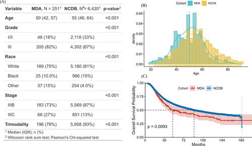
Our goal is to borrow IBC patient data from NCDB (source cohort) to improve the individualized risk estimation of MD Anderson patients (target cohort). The observations from Figure 4 suggest a possible referral bias for data from large cancer cancers, such as MD Anderson, in which patients tend to be sicker than the general IBC patients represented by NCDB. Meanwhile, due to the substantial differences in mortality risk between the two cohorts, it is not appropriate to directly merge the two cohorts for the inference of the MDA cohort.

We apply both the proposed Trans-Cox algorithm and conventional Cox regression on the MDA and NCDB cohorts. Table 1 shows the estimated coefficients (log hazard ratios) from the five methods: Trans-Cox with MDA as the target cohort and NCDB as the source cohort, Cox model with MDA only, Cox model with NCDB only, Cox model with the combined data of MDA and NCDB, and Cox model stratified by the data sources. Age is standardized in both datasets (Figure S6). There are several interesting observations. First, the Cox model with the simple combined data and stratified approach has almost identical inference results as the Cox model with NCDB data only. This illustrates that when the sample size of the source cohort is much larger than the target cohort (6420 vs. 251), the estimation results of the combined cohort are dominated by the source cohort. This observation is also confirmed by the estimation of cumulative baseline hazards presented in Figure S7 in which the estimated cumulative baseline hazards using the combined cohort are almost identical to those using NCDB only. Figure S8 shows the sparsity of the estimated η and ξ by TransCox. We observe that one estimated η (for “Race:Other vs. White”) and several ξ estimators are close to zero, indicating that the coefficient information of other Race group and the cumulative baseline hazards at those time points are mostly borrowed from the source cohort by Trans-Cox.

Table 1 Analysis results of the MDA and NCDB cohorts.

$\widehat{\beta }$
	Trans-Cox	Cox(MDA)	Cox(NCDB)	Cox(Combined) ${}^{\mathrm{d}}a\mathit{gger}$	Cox(Stratified)
Normalized Age	0.091	0.074	0.208	0.197	0.199
Grade:III vs. I/II	0.616	0.388	0.347	0.353	0.348
Race:Black vs. White	0.272	0.163	0.429	0.412	0.416
Race:Other vs. White	−0.128	−0.336	−0.113	−0.107	−0.130
Stage:IIIC vs. IIIB	−0.059	−0.243	0.386	0.368	0.357
Trimodality:Yes vs. No	−0.838	−1.174	−0.589	−0.636	−0.627
SE ${}^{*}$
	Trans-Cox	Cox(MDA)	Cox(NCDB)	Cox(Combined)	Cox(Stratified)
Normalized Age	0.121	0.109	0.021	0.021	0.021
Grade:III vs. I/II	0.197	0.269	0.044	0.043	0.044
Race:Black vs. White	0.265	0.325	0.051	0.051	0.051
Race:Other vs. White	0.261	0.295	0.118	0.109	0.109
Stage:IIIC vs. IIIB	0.179	0.244	0.055	0.053	0.054
Trimodality:Yes vs. No	0.207	0.230	0.069	0.065	0.065
p-value
	Trans-Cox	Cox(MDA)	Cox(NCDB)	Cox(Combined)	Cox(Stratified)
Normalized age	0.453	0.498	¡0.001	¡0.001	¡0.001
Grade:III vs. I/II	0.002	0.150	¡0.001	¡0.001	¡0.001
Race:Black vs. White	0.305	0.616	¡0.001	¡0.001	¡0.001
Race:Other vs. White	0.623	0.295	0.118	0.109	0.19
Stage:IIIC vs. IIIB	0.753	0.318	¡0.001	¡0.001	¡0.001
Trimodality:Yes vs. No	¡0.001	¡0.001	¡0.001	¡0.001	¡0.001

${}^{\ast }$ Boostrap-based standard error estimation with 1000 bootstrap resamplings. ${}^{\mathrm{d}ag}$ Cox(Combined) is the Cox regression model using the combined data of MDA and NCDB.

Second, some covariates have similar effect sizes, while others have quite different effect sizes on survival between the two cohorts. The Cox model based on the MDA cohort has similar effect sizes for age and grade, but has a much smaller effect for the race being Black compared to the effect size estimated using the NCDB cohort. Rueth et al. (2014) reported that the Black population tended to be treated not according to the IBC treatment guidelines compared to the White IBC patients, thus, increasing the mortality risk of Black patients in NCDB. However, breast cancer patients treated at MD Anderson generally received their treatment according to the guidelines regardless of their racial background (Shen et al. 2007). As a result, racial status plays a less influential role in the MDA cohort than in the NCDB cohort.

Third, we observe that Trans-Cox can effectively transfer knowledge on the regression coefficients from the NCDB cohort to the MDA cohort for similar effects and simultaneously reduce information borrowing for inconsistent effects. In the upper panel of Table 1, the estimated standard errors of grade and trimodality are substantially reduced, resulting in more precise estimators compared to the Cox model using the MDA cohort alone. Different from other subtypes of breast cancer, all IBC started as Stage III since they involve the skin. Both data cohorts focus only on Stage III IBC patients with a fine category of B versus C. The stage (Stage IIIB vs. Stage IIIC) has a nonsignificant effect on overall survival by using the MDA cohort only or borrowing information from NCDB with Trans-Cox. The standard errors of the parameters and the 95% confidence intervals of the Trans-Cox method are obtained using bootstrap.

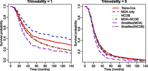
We also estimate the survival curves for patients with or without receiving trimodality and present the results in Figure 5. The left panel shows the estimated survival curve for Black patients with age 50, grade III, stage IIIC, and receiving trimodality. We find that patients receiving trimodality treatment at MD Anderson have better survival outcomes compared to IBC patients with the same baseline characteristics even after Trans-Cox borrows information from NCDB. This suggests that MD Anderson may provide better care than the average medical institution in the United States. The right panel contains the survival curves for the patient with the same characteristics (Black, age 50, grade III, stage IIIC) but without receiving trimodality treatment. It is interesting that patients did not have any survival benefit even if they were treated at MD Anderson Cancer Center without using trimodality.

Fig. 5 The estimated survival curves using different methods for patients with (left panel) or without (right panel) receiving trimodality treatment. Other characteristics were specified as: age 50 years old, grade III, Black race, and stage IIIC.

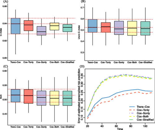
Lastly, we evaluate the prediction performance of fitted models using the concordance index (C-index) (Steck et al. 2007), Uno’s C-index (Uno et al. 2011), area under the receiver operating characteristic curve (AUC), and error of estimated personalized risk prediction (Uno et al. 2007). The error of estimated personalized risk prediction at time L is defined as ${\sum }_{i=1}^N{\widehat{w}}_i\{{\widehat{p}}_i(L)-1(Y_i\ge L)\}/{\sum }_{i=1}^N{\widehat{w}}_i$ where ${\widehat{w}}_i=\frac{1(Y_i\le L){\delta }_i}{\widehat{G}(Y_i)}+\frac{1(Y_i\ge L)}{\widehat{G}(L)}$ and $\widehat{G}$ is the Kaplan-Meier estimation function of the censored time $\left\{C_i\right\}$. We evaluate the personalized risk prediction at time points $L=\{20,30,\dots ,110\}$. We use the bootstrap-based method to evaluate the survival risk prediction for the MDA data and compare with the true observations (Steyerberg et al. 2001). Figure 6 shows that the Trans-Cox model outperforms the Cox model using the target data only (“Cox-Tonly” in Figure 6) in terms of estimation precision, while both methods exhibit similar predictive performance, as measured by Uno’s C index. The Cox model using the combined cohort (“Cox-Both”), the stratified Cox model (“Cox-Stratified”), and the Cox model using the source cohort, NCDB, alone (“Cox-Sonly”) have similarly poor performance. Overall, the Trans-Cox and Cox-Tonly models have the best prediction accuracy, while the other three models (Cox-Sonly, Cox-Both, Cox-Stratified) have lower concordances and higher prediction errors.

Fig. 6 Evaluation of the prediction performance of four methods using C-index (Panel A), Uno’s C-index (B), AUC (C), and personalized risk prediction error (D).

5 Discussion

Motivated by the challenges in borrowing information from a source cohort to improve the time-varying risk assessment for a target cohort, this article develops a transfer learning-based method that adaptively determines the degree of information transferring from the source cohort. Previous works that combine multiple data sources often need to consider the covariate distribution shift between the study cohorts, for example, when estimating marginal treatment effects or generalizing research findings to a larger population (Colnet et al. 2020; Wu and Yang 2021). Our problem focuses on individual risk assessment and does not need to address such covariate distribution shifts. The proposed method can naturally address the heterogeneity between the two cohorts by imposing L-1 penalties. Much of the literature has a developed adaptive Lasso for the Cox model to allow feature selection (Tibshirani 1997; Zhang and Lu 2007). Different from these methods, our Trans-Cox model imposes the Lasso penalty on the discrepancy in regression coefficients and baseline hazard functions between the two resources. Our model considers the penalties from both sides in a unified framework to allow simultaneous control of the information sharing for the covariate effects and time-varying baseline hazards under the Cox model.

Bayesian methods may appear to be a natural modeling strategy to borrowing information from the source cohort to improve the estimation in the target cohort. However, there are several challenges to solve the current problem using a standard Bayesian approach. First, when the ratio of sample sizes of the two cohorts is large, the posterior distribution would be dominated by the source cohort if directly fitting the two cohorts with Bayesian methods, although the risk estimation for the target cohort is the purpose. To solve this, a few tuning parameters may need to be involved and carefully selected to balance the sample sizes and heterogeneity between the two cohorts. Second, besides the nonparametric component under the Cox model, the dimension of η and ξ increases with the sample size as well, which also increases the computational cost for a Bayesian approach.

A fundamental assumption of many previous works that borrow information from the source population is the comparability between the two cohorts (Chatterjee et al. 2016; Li et al. 2022). Our method relaxes this assumption by accommodating situations when the two cohorts can be heterogeneous. Such heterogeneity commonly exists in practice due to various types of selection biases, demographic differences, regulatory restrictions, etc. As shown in our results, when the risk models of the two cohorts are different, directly combining the two datasets can result in biased findings. This estimation bias can be substantial when the sample size of the source cohort is much larger than the target cohort. In contrast, Trans-Cox demonstrates robust estimations even when there are high levels of cohort heterogeneity. This highlights the significance of our research question and the proposed methodology.

Moreover, many recent studies have discussed the challenges of sharing individual-level data in multi-site studies due to feasibility, privacy, and other concerns (Maro et al. 2009; Toh et al. 2011; Li et al. 2019). The existing transfer learning and information borrowing methods usually adapt their proposals to incorporate the summary statistics from the source cohort in the analysis, replacing the need of individual-level data for the source population (Chatterjee et al. 2016; Li et al. 2022). But none of the work is directly applicable to time-to-event data or allows time varying differences in baseline hazards of the two cohorts. We also recognize the importance of this issue and allow Trans-Cox to directly incorporate summary statistics of estimated coefficients and cumulative baseline hazards as the information from the source cohort. This advantage facilitates the use of information from additional sources with the guarantee of protecting patient privacy.

It is worth noting that the primary purpose of using the L-1 penalty in our method is not to control sparsity, but to regulate the amount of information borrowed from the source cohort to the target cohort. The L-1 penalty has been successfully used in the literature to control information discrepancy (Chen et al. 2021; Ding et al. 2023). We employ the L-1 penalty to control the distance in the cumulative baseline hazard component ($\mathit{\xi }$) due to the high dimension of the failure time points. We also apply it to the covariate coefficient component ($\mathit{\eta }$) for consistency, although other types of penalty could also be used for such a purpose. When high-dimensional covariates are present, feature selection must be incorporated into our proposed method. One simple solution is to add an additional L-1 penalty component on $\mathit{\beta }$, but the implementation details are beyond the scope of this work.

The proposed method can be extended in several ways. First, the current framework only considers point estimators from the source cohort. When the source cohort has a large sample size, for example in the NCDB data, the estimation variations are negligible. However, the estimation uncertainties can be nonnegligible when a smaller or more diverse source cohort is considered. Incorporating such uncertainties in the method may better inform the level of knowledge sharing between the cohorts and further improve accuracy.

Second, we focus on the situation where one source cohort is available. Although the current method can be directly extended to multiple source situations by combining all the source data as a single source cohort, this naive extension may over-simplify the complexity of this problem. For example, when there are different directions of the covariate effects and large variations in sample sizes among multiple sources, it is unclear how to achieve the balance between the estimation accuracy and the model flexibility. Li, Cai, and Li (2020) discussed approaches to identify informative auxiliary cohorts and aggregate these cohorts to improve transfer learning in the high-dimensional linear regression setting. Similar approaches can be considered here to allow for incorporating the information from multiple source populations.

Third, similar to several existing methods (Dahabreh et al. 2020), we assume the interested covariates are available for both cohorts. This could be a limitation in practice as medical institutions or clinical trials sometimes capture different covariates from the population-level data registries (Taylor, Choi, and Han 2022). Further extensions can be made to allow for incorporating a subset of regression coefficients to improve individualized risk assessment. Finally, it is generally believed that a standard bootstrap may not work well in the regression problem using L₁ penalization (Chatterjee and Lahiri 2011). Although our simulation study demonstrates a reasonable performance for the bootstrap-based inference, the evaluation is restricted by the simulation settings. We acknowledge that the theoretical justification for the inference procedure is beyond the scope of this work and worthy of future research.

Supplementary Materials

Supplementary: this file includes Figures S1–S9 and Tables S1–S3. (pdf)

R-package for Trans-Cox implementation: R-package TransCox is publicly available from https://github.com/ziyili20/TransCox with a detailed user manual and example. The code to reproduce the simulation figures and results in the manuscript is provided through https://github.com/ziyili20/TransCox/_reproduceFigures.

Acknowledgments

The authors wish to thank Dr. Naoto Ueno and his team for sharing IBC patient cohort data, and Dr. Isabelle Bedrosain and the team for collaboration on the NCDB project, which motivated this research. The authors acknowledge the helpful comments from the editor, associate editor, and two anonymous reviewers in improving the manuscript. The authors also acknowledge Ms. Jessica T. Swann from MD Anderson for her help in language editing.

Additional information

Funding

This work is supported by the National Institutes of Health (R01CA269696 and R03CA270725).

References

- Antonelli, J., Zigler, C., and Dominici, F. (2017), “Guided Bayesian Imputation to Adjust for Confounding When Combining Heterogeneous Data Sources in Comparative Effectiveness Research,” Biostatistics, 18, 553–568. DOI: 10.1093/biostatistics/kxx003.
- Bilimoria, K. Y., Stewart, A. K., Winchester, D. P., and Ko, C. Y. (2008), “The National Cancer Data Base: A Powerful Initiative to Improve Cancer Care in the United States,” Annals of Surgical Oncology, 15, 683–690. DOI: 10.1245/s10434-007-9747-3.
- Breslow, N. E. (1972), “Contribution to Discussion of Paper by DR Cox,” Journal of the Royal Statistical Society, Series B, 34, 216–217.
- Burnham, K. P., and Anderson, D. R. (2004), “Multimodel Inference: Understanding AIC and BIC in Model Selection,” Sociological Methods & Research, 33, 261–304. DOI: 10.1177/0049124104268644.
- Cai, T. T., and Wei, H. (2021), “Transfer Learning for Nonparametric Classification: Minimax Rate and Adaptive Classifier,” The Annals of Statistics, 49, 100–128. DOI: 10.1214/20-AOS1949.
- Carlé, A., Pedersen, I. B., Perrild, H., Ovesen, L., Jørgensen, T., and Laurberg, P. (2013), “High Age Predicts Low Referral of Hyperthyroid Patients to Specialized Hospital Departments: Evidence for Referral Bias,” Thyroid, 23, 1518–1524. DOI: 10.1089/thy.2013.0074.
- Carvalho, A. L., Nishimoto, I. N., Califano, J. A., and Kowalski, L. P. (2005), “Trends in Incidence and Prognosis for Head and Neck Cancer in the United States: A Site-Specific Analysis of the Seer Database,” International Journal of Cancer, 114, 806–816. DOI: 10.1002/ijc.20740.
- Chatterjee, N., Chen, Y.-H., Maas, P., and Carroll, R. J. (2016), “Constrained Maximum Likelihood Estimation for Model Calibration Using Summary-Level Information from External Big Data Sources,” Journal of the American Statistical Association, 111, 107–117. DOI: 10.1080/01621459.2015.1123157.
- Chatterjee, A., and Lahiri, S. N. (2011), “Bootstrapping Lasso Estimators,” Journal of the American Statistical Association, 106, 608–625. DOI: 10.1198/jasa.2011.tm10159.
- Chen, Z., Ning, J., Shen, Y., and Qin, J. (2021), “Combining Primary Cohort Data with External Aggregate Information without Assuming Comparability,” Biometrics, 77, 1024–1036. DOI: 10.1111/biom.13356.
- Colnet, B., Mayer, I., Chen, G., Dieng, A., Li, R., Varoquaux, G., Vert, J.-P., Josse, J., and Yang, S. (2020), “Causal Inference Methods for Combining Randomized Trials and Observational Studies: A Review,” arXiv preprint arXiv:2011.08047.
- Cox, D. R. (1972), “Regression Models and Life-Tables,” Journal of the Royal Statistical Society, Series B, 34, 187–202. DOI: 10.1111/j.2517-6161.1972.tb00899.x.
- Dahabreh, I. J., Robertson, S. E., Steingrimsson, J. A., Stuart, E. A., and Hernan, M. A. (2020), “Extending Inferences from a Randomized Trial to a New Target Population,” Statistics in Medicine, 39, 1999–2014. DOI: 10.1002/sim.8426.
- Dillon, J. V., Langmore, I., Tran, D., Brevdo, E., Vasudevan, S., Moore, D., Patton, B., Alemi, A., Hoffman, M., and Saurous, R. A. (2017), “Tensorflow Distributions,” arXiv preprint arXiv:1711.10604.
- Ding, J., Li, J., Han, Y., McKeague, I. W., and Wang, X. (2023), “Fitting Additive Risk Models Using Auxiliary Information,” Statistics in Medicine, 42, 894–916. DOI: 10.1002/sim.9649.
- Dürr, O., Sick, B., and Murina, E. (2020), Probabilistic Deep Learning: With Python, Keras and Tensorflow Probability, Shelter Island, NY: Manning Publications.
- Huang, C.-Y., Qin, J., and Tsai, H.-T. (2016), “Efficient Estimation of the Cox Model with Auxiliary Subgroup Survival Information,” Journal of the American Statistical Association, 111, 787–799. DOI: 10.1080/01621459.2015.1044090.
- Jaiyesimi, I. A., Buzdar, A. U., and Hortobagyi, G. (1992), “Inflammatory Breast Cancer: A Review,” Journal of Clinical Oncology, 10, 1014–1024. DOI: 10.1200/JCO.1992.10.6.1014.
- Jeong, S., and Namkoong, H. (2020), “Robust Causal Inference Under Covariate Shift via Worst-Case Subpopulation Treatment Effects,” in Conference on Learning Theory, pp. 2079–2084, PMLR.
- Jiao, F. F., Fung, C. S. C., Wan, E. Y. F., Chan, A. K. C., McGhee, S. M., Kwok, R. L. P., and Lam, C. L. K. (2018), “Five-Year Cost-Effectiveness of the Multidisciplinary Risk Assessment and Management Programme–Diabetes Mellitus (RAMP-DM),” Diabetes Care, 41, 250–257. DOI: 10.2337/dc17-1149.
- Karr, A. F., Fulp, W. J., Vera, F., Young, S. S., Lin, X., and Reiter, J. P. (2007), “Secure, Privacy-Preserving Analysis of Distributed Databases,” Technometrics, 49, 335–345. DOI: 10.1198/004017007000000209.
- Kumar, A., Guss, Z. D., Courtney, P. T., Nalawade, V., Sheridan, P., Sarkar, R. R., Banegas, M. P., Rose, B. S., Xu, R., and Murphy, J. D. (2020), “Evaluation of the Use of Cancer Registry Data for Comparative Effectiveness Research,” JAMA Network Open, 3, e2011985Z. DOI: 10.1001/jamanetworkopen.2020.11985.
- Li, D., Lu, W., Shu, D., Toh, S., and Wang, R. (2022), “Distributed Cox Proportional Hazards Regression Using Summary-Level Information,” Biostatistics, kxac006. DOI: 10.1093/biostatistics/kxac006.
- Li, J., Panucci, G., Moeny, D., Liu, W., Maro, J. C., Toh, S., and Huang, T.-Y. (2018), “Association of Risk for Venous Thromboembolism with Use of Low-Dose Extended-and Continuous-Cycle Combined Oral Contraceptives: A Safety Study Using the Sentinel Distributed Database,” JAMA Internal Medicine, 178, 1482–1488. DOI: 10.1001/jamainternmed.2018.4251.
- Li, S., Cai, T., and Duan, R. (2021), “Targeting Underrepresented Populations in Precision Medicine: A Federated Transfer Learning Approach,” arXiv preprint arXiv:2108.12112.
- Li, S., Cai, T. T., and Li, H. (2020), “Transfer Learning for High-Dimensional Linear Regression: Prediction, Estimation, and Minimax Optimality,” arXiv preprint arXiv:2006.10593.
- Li, S., Cai, T. T., and Li, H. (2022), “Transfer Learning in Large-Scale Gaussian Graphical Models with False Discovery Rate Control,” Journal of the American Statistical Association, 1–13. DOI: 10.1080/01621459.2022.2044333.
- Li, Z., Roberts, K., Jiang, X., and Long, Q. (2019), “Distributed Learning from Multiple EHR Databases: Contextual Embedding Models for Medical Events,” Journal of Biomedical Informatics, 92, 103138. DOI: 10.1016/j.jbi.2019.103138.
- Liauw, S. L., Benda, R. K., Morris, C. G., and Mendenhall, N. P. (2004), “Inflammatory Breast Carcinoma: Outcomes with Trimodality Therapy for Nonmetastatic Disease,” Cancer, 100, 920–928. DOI: 10.1002/cncr.20083.
- Lin, D.-Y., and Zeng, D. (2010), “On the Relative Efficiency of Using Summary Statistics Versus Individual-Level Data in Meta-Analysis,” Biometrika, 97, 321–332. DOI: 10.1093/biomet/asq006.
- Liu, D., Zheng, Y., Prentice, R. L., and Hsu, L. (2014), “Estimating Risk with Time-to-Event Data: An Application to the Women’s Health Initiative,” Journal of the American Statistical Association, 109, 514–524. DOI: 10.1080/01621459.2014.881739.
- Maro, J. C., Platt, R., Holmes, J. H., Strom, B. L., Hennessy, S., Lazarus, R., and Brown, J. S. (2009), “Design of a National Distributed Health Data Network,” Annals of Internal Medicine, 151, 341–344. DOI: 10.7326/0003-4819-151-5-200909010-00139.
- Masuda, H., Brewer, T., Liu, D., Iwamoto, T., Shen, Y., Hsu, L., Willey, J., Gonzalez-Angulo, A., Chavez-MacGregor, M., Fouad, T., et al. (2014), “Long-Term Treatment Efficacy in Primary Inflammatory Breast Cancer by Hormonal Receptor-and HER2-Defined Subtypes,” Annals of Oncology, 25, 384–391. DOI: 10.1093/annonc/mdt525.
- Neath, A. A., and Cavanaugh, J. E. (2012), “The Bayesian Information Criterion: Background, Derivation, and Applications,” Wiley Interdisciplinary Reviews: Computational Statistics, 4, 199–203. DOI: 10.1002/wics.199.
- Platt, J., and Kardia, S. (2015), “Public Trust in Health Information Sharing: Implications for Biobanking and Electronic Health Record Systems,” Journal of Personalized Medicine, 5, 3–21. DOI: 10.3390/jpm5010003.
- Raval, M. V., Bilimoria, K. Y., Stewart, A. K., Bentrem, D. J., and Ko, C. Y. (2009), “Using the NCDB for Cancer Care Improvement: An Introduction to Available Quality Assessment Tools,” Journal of Surgical Oncology, 99, 488–490. DOI: 10.1002/jso.21173.
- Rueth, N. M., Lin, H. Y., Bedrosian, I., Shaitelman, S. F., Ueno, N. T., Shen, Y., and Babiera, G. (2014), “Underuse of Trimodality Treatment Affects Survival for Patients with Inflammatory Breast Cancer: An Analysis of Treatment and Survival Trends from the National Cancer Database,” Journal of Clinical Oncology, 32, 2018–2024. DOI: 10.1200/JCO.2014.55.1978.
- Shen, Y., Dong, W., Esteva, F. J., Kau, S.-W., Theriault, R. L., and Bevers, T. B. (2007), “Are There Racial Differences in Breast Cancer Treatments and Clinical Outcomes for Women Treated at MD Anderson Cancer Center?” Breast Cancer Research and Treatment, 102, 347–356. DOI: 10.1007/s10549-006-9337-2.
- Steck, H., Krishnapuram, B., Dehing-Oberije, C., Lambin, P., and Raykar, V. C. (2007), “On Ranking in Survival Analysis: Bounds on the Concordance Index,” in Advances in Neural Information Processing Systems (Vol. 20).
- Steyerberg, E. W., Harrell Jr, F. E., Borsboom, G. J., Eijkemans, M., Vergouwe, Y., and Habbema, J. D. F. (2001), “Internal Validation of Predictive Models: Efficiency of Some Procedures for Logistic Regression Analysis,” Journal of Clinical Epidemiology, 54, 774–781. DOI: 10.1016/s0895-4356(01)00341-9.
- Sugiyama, M., Krauledat, M., and Müller, K.-R. (2007), “Covariate Shift Adaptation by Importance Weighted Cross Validation,” Journal of Machine Learning Research, 8, 985–1005.
- Taylor, J. M., Choi, K., and Han, P. (2022), “Data Integration: Exploiting Ratios of Parameter Estimates from a Reduced External Model,” Biometrika, 110, 119–134. DOI: 10.1093/biomet/asac022.
- Tian, Y., and Feng, Y. (2022), “Transfer Learning Under High-Dimensional Generalized Linear Models,” Journal of the American Statistical Association, 1–30, DOI: 10.1080/01621459.2022.207127.8.
- Tibshirani, R. (1997), “The Lasso Method for Variable Selection in the Cox Model,” Statistics in Medicine, 16, 385–395. DOI: 10.1002/(SICI)1097-0258(19970228)16:4<385::AID-SIM380>3.0.CO;2-3.
- Toh, S. (2020), “Analytic and Data Sharing Options in Real-World Multidatabase Studies of Comparative Effectiveness and Safety of Medical Products,” Clinical Pharmacology & Therapeutics, 107, 834–842. DOI: 10.1002/cpt.1754.
- Toh, S., Platt, R., Steiner, J., and Brown, J. (2011), “Comparative-Effectiveness Research in Distributed Health Data Networks,” Clinical Pharmacology & Therapeutics, 90, 883–887. DOI: 10.1038/clpt.2011.236.
- Uno, H., Cai, T., Pencina, M. J., D’Agostino, R. B., and Wei, L.-J. (2011), “On the C-statistics for Evaluating Overall Adequacy of Risk Prediction Procedures with Censored Survival Data,” Statistics in Medicine, 30, 1105–1117. DOI: 10.1002/sim.4154.
- Uno, H., Cai, T., Tian, L., and Wei, L.-J. (2007), “Evaluating Prediction Rules for t-year Survivors with Censored Regression Models,” Journal of the American Statistical Association, 102, 527–537. DOI: 10.1198/016214507000000149.
- Van Uden, D., Van Laarhoven, H., Westenberg, A., de Wilt, J., and Blanken-Peeters, C. (2015), “Inflammatory Breast Cancer: An Overview,” Critical Reviews in Oncology/Hematology, 93, 116–126. DOI: 10.1016/j.critrevonc.2014.09.003.
- Wu, L., and Yang, S. (2021), “Transfer Learning of Individualized Treatment Rules from Experimental to Real-World Data,” arXiv preprint arXiv:2108.08415. DOI: 10.1080/10618600.2022.2141752.
- Zhang, H. H., and Lu, W. (2007), “Adaptive Lasso for Cox’s Proportional Hazards Model,” Biometrika, 94, 691–703. DOI: 10.1093/biomet/asm037.