Narrowest Significance Pursuit: Inference for Multiple Change-Points in Linear Models

Abstract

We propose Narrowest Significance Pursuit (NSP), a general and flexible methodology for automatically detecting localized regions in data sequences which each must contain a change-point (understood as an abrupt change in the parameters of an underlying linear model), at a prescribed global significance level. NSP works with a wide range of distributional assumptions on the errors, and guarantees important stochastic bounds which directly yield exact desired coverage probabilities, regardless of the form or number of the regressors. In contrast to the widely studied “post-selection inference” approach, NSP paves the way for the concept of “post-inference selection.” An implementation is available in the R package nsp. Supplementary materials for this article are available online.

KEYWORDS:

• Confidence intervals
• Narrowest-over-threshold
• Post-selection inference
• Structural breaks
• Wild binary segmentation

1 Introduction

We propose a new generic methodology for determining, for a given data sequence and at a given global significance level, localized regions of the data that each must contain a change-point. We define a change-point in $Y_t$ on an interval [s, e] as an abrupt departure, on that interval, from a linear model for $Y_t$ with respect to pre-specified regressors. We now give examples of scenarios covered by the proposed methodology.

Scenario 1.

Piecewise-constant signal plus noise model. (1) $$Y_t=f_t+Z_t,\hspace{1em}t=1,\dots ,T,$$(1) where $f_t$ is a piecewise-constant vector with an unknown number N and locations $0={\eta }_0<{\eta }_1<\cdots <{\eta }_N<{\eta }_{N+1}=T$ of change-points, and $Z_t$ is zero-centered noise. The location ${\eta }_j$ is a change-point if $f_{{\eta }_j-1}=f_{{\eta }_j}$ but $f_{{\eta }_j}\ne f_{{\eta }_j+1}$.

Scenario 2.

Piecewise-polynomial (e.g., piecewise-constant or piecewise-linear) signal plus noise model. In (1), $f_t$ is a piecewise-polynomial vector, in which the polynomial pieces have a fixed degree $q\ge 0$, assumed known to the analyst. The location ${\eta }_j$ is a change-point if $f_t$ can be described as a polynomial vector of degree q on $[{\eta }_j-q-1,{\eta }_j]$, but not on $[{\eta }_j-q,{\eta }_j+1]$.

Scenario 3.

Linear regression with piecewise-constant parameters. For a given design matrix $X=(X_{t,i})$, $t=1,\dots ,T$, $i=1,\dots ,p$, the response $Y_t$ follows the model (2) $$Y_t=X_{t,\cdot }{\beta }^{(j)}+Z_t\hspace{1em}\text{for}\hspace{1em}t={\eta }_j+1,\dots ,{\eta }_{j+1},\hspace{1em}j=0,\dots ,N,$$(2) where the parameter vectors ${\beta }^{(j)}={({\beta }_1^{(j)},\dots ,{\beta }_p^{(j)})}^{\prime }$ are such that ${\beta }^{(j)}\ne {\beta }^{(j+1)}$.

Each of these scenarios is a generalization of the preceding one. We permit a broad range of distributional assumptions for $Z_t$, from iid Gaussianity to autocorrelation, heavy tails and heterogeneity. We now review the existing literature on uncertainty in multiple change-point problems which seeks to make confidence statements about the existence or locations of change-points in particular regions of the data, or significance statements about their importance.

In the iid Gaussian piecewise-constant model, SMUCE (Frick, Munk, and Sieling 2014) estimates the number N of change-points as the minimum among those candidate fits ${\widehat{f}}_t$ for which the empirical residuals pass a certain test at level $\alpha$. An issue for SMUCE, discussed for example in Chen, Shah, and Samworth (2014), is that the smaller the significance level $\alpha$, the more lenient the test on the empirical residuals, and therefore the higher the risk of underestimating N. This leads to the counter-intuitive behavior of the coverage properties of SMUCE illustrated in Chen, Shah, and Samworth (2014). SMUCE2 (Chen, Shah, and Samworth 2014) remedies this issue, but still requires that the number of estimated change-points agrees with the truth for successful coverage, which puts it at risk of being unable to cover the truth with a high nominal probability requested by the user. In the approach taken in this article, this issue does not arise as we shift the inferential focus away from N. SMUCE is extended to heterogeneous Gaussian noise in Pein, Sieling, and Munk (2017) and to dependent data in Dette, Eckle, and Vetter (2020).

Some authors approach uncertainty quantification for multiple change-point problems from the point of view of post-selection inference (PSI, a.k.a. selective inference); these include Hyun, G’Sell, and Tibshirani (2018), Hyun et al. (2021), Jewell, Fearnhead, and Witten (2022), and Duy et al. (2020). To ensure valid inference, PSI conditions on many aspects of the estimation process, which tends to produce p-values with somewhat complex definitions. PSI also does not permit the selection of the tuning parameters of the inference procedure from the same data. Useful as they are in assessing the significance of previously estimated change-points, these PSI approaches share the following features: (a) they do not consider uncertainties in estimating change-point locations, (b) they do not provide regions of globally significant change in the data, (c) they define significance for each change-point separately, as opposed to globally, (d) they rely on a particular base change-point detection method with its potential strengths or weaknesses. Our approach contrasts with these features; in particular, in contrast to PSI, it can be described as enabling “post-inference selection,” as we argue later on.

Some authors provide simultaneous asymptotic distributional results for the distance between the estimated change-point locations and the truth. In the linear regression context, this is done in Bai and Perron (1998), Bai and Perron (2003), and in the piecewise-constant signal plus noise model—in Eichinger and Kirch (2018). These approaches are asymptotic, conditional on the estimated change-point locations, and involve unknown quantities. In contrast, our methodology has a finite-sample nature, makes no assumptions on the signal, is unconditional and automatic. A further discussion of the differences between our approach and that of Bai and Perron (1998), Bai and Perron (2003) can be found in Section 1 of the supplement.

Inference for multiple change-points is also sometimes posed as control of the False Discovery Rate (FDR), see for example, Li and Munk (2016), Hao, Niu, and Zhang (2013), and Cheng, He, and Schwartzman (2020), but that approach is focused on the number of change-points rather than on their locations.

The objective of our methodology, called “Narrowest Significance Pursuit” (NSP), is to automatically detect localized regions of the data $Y_t$, each of which must contain at least one change-point (in a suitable sense determined by the given scenario), at a prescribed global significance level. NSP performs unconditional inference without change-point location estimation, and proceeds as follows. A number M of intervals are drawn from the index domain $[1,\dots ,T]$, with start- and end-points chosen over an equispaced deterministic grid. On each interval drawn, $Y_t$ is then checked to see whether or not it locally conforms to the prescribed linear model, with any set of parameters. This check is performed through estimating the parameters of the given linear model locally by minimizing a particular multiresolution sup-norm loss, and testing the residuals from this fit via the same norm; self-normalization is involved if necessary. In the first greedy stage, the shortest interval (if one exists) is chosen on which the test is violated at a certain global significance level $\alpha$. In the second greedy stage, the selected interval is searched for its shortest sub-interval on which a similar test is violated. This sub-interval is then chosen as the first region of global significance, in the sense that it must (at a global level $\alpha$) contain a change-point, or otherwise the local test would not have rejected the linear model. The procedure then recursively draws M intervals to the left and to the right of the chosen region (with or without overlap), and stops when there are no further local regions of global significance.

Fang, Li, and Siegmund (2020), in the piecewise-constant signal plus iid Gaussian noise model, approximate the tail probability of the maximum CUSUM statistic over all sub-intervals of the data. They then propose an algorithm, in a few variants, for identifying short, nonoverlapping segments of the data on which the local CUSUM exceeds the derived tail bound, and hence, the segments identified must contain at least a change-point each, at a given significance level. Fang and Siegmund (2020) present results of similar nature for a Gaussian model with lag-one autocorrelation, linear trend, and features that are linear combinations of continuous, piecewise differentiable shapes. The most important high-level differences between NSP and these two approaches are that (a) NSP is ready for use with any user-provided design matrix X, and this requires no new calculations or coding, and yields correct coverage probabilities in finite samples of any length; (b) NSP searches for any deviations from local model linearity with respect to the regressors provided; (c) NSP is able to handle regression with autoregression practically in the same way as without, in a stable manner and on arbitrarily short intervals, and does not need accurate estimation of the unknown (nuisance) AR coefficients. We expand on these points in Section 1 of the supplement.

NSP has other distinctive features in comparison with the existing literature. It is specifically constructed to target the shortest possible significant intervals at every stage of the procedure, and to explore as many intervals as possible while remaining computationally efficient. NSP furnishes exact coverage statements, at a prescribed global significance level, for any finite sample sizes, and works in the same way regardless of the scenario and for any given regressors X. Also, thanks to the fact that the multiresolution sup-norm used in NSP can be interpreted as Hölder-like norms on certain function spaces, NSP naturally extends to the cases of unknown or heterogeneous distributions of $Z_t$ via self-normalization. Finally, if simulation needs to be used to determine critical values for NSP, then this can be done in a computationally efficient manner.

Section 2 introduces the NSP methodology and provides the relevant finite-sample coverage theory. Section 3 extends this to NSP under self-normalization and in the additional presence of autoregression. Section 4 provides finite-sample and traditional large-sample detection consistency and rate optimality results for NSP in Scenarios 1 and 2. Section 5 provides comparative simulations and extensive numerical examples under a variety of settings. Section 6 describes two real-data case studies. Complete R code implementing NSP is available in the R package nsp. There is a supplement, whose contents are mentioned at appropriate places in the article. Proofs of our theoretical results are in the supplement.

2 The NSP Inference framework

Throughout the section, we use the language of Scenario 3, which includes Scenarios 1 and 2 as special cases. In Scenario 1, the matrix X in (2) is of dimensions $T\times 1$ and has all entries equal to 1. In Scenario 2, the matrix X is of dimensions $T\times (q+1)$ and its ith column is given by ${(t/T)}^{i-1}$, $t=1,\dots ,T$. Scenario 4 (for NSP in the additional presence of autoregression), which generalizes Scenario 3, is handled with in Section 3.2.

2.1 Generic NSP Algorithm

We start with a pseudocode definition of the NSP algorithm, in the form of a recursively defined function NSP. In its arguments, [s, e] is the current interval under consideration and at the start of the procedure, we have $[s,e]=[1,T]$; Y (of length T) and X (of dimensions $T\times p$) are as in the model formula (2); M is the number of sub-intervals of [s, e] drawn; ${\lambda }_{\alpha }$ is the threshold corresponding to the global significance level $\alpha$ (typical values for $\alpha$ would be 0.05 or 0.1) and ${\tau }_L$ (respectively ${\tau }_R$) is a functional parameter used to specify the degree of overlap of the left (respectively right) child interval of [s, e] with respect to the region of significance identified within [s, e], if any. The no-overlap case would correspond to ${\tau }_L={\tau }_R\equiv 0$. In each recursive call on a generic interval [s, e], NSP adds to the set $\mathcal{S}$ any globally significant local regions (intervals) of the data identified within [s, e] on which Y is deemed to depart significantly (at global level $\alpha$) from linearity with respect to X. We provide more details underneath the pseudocode below.

1: function NSP(s, e, Y, X, M, ${\lambda }_{\alpha }$, ${\tau }_L$, ${\tau }_R$)

2: if $e-s<1$ then

3: RETURN

4: end if

5: if $M\ge \frac{1}{2}(e-s+1)(e-s)$ then

6: $M:=\frac{1}{2}(e-s+1)(e-s)$

7: draw all intervals $[s_m,e_m]\subseteq [s,s+1,\dots ,e]$, $m=1,\dots ,M$, s.t. $e_m-s_m\ge 1$

8: else

9: draw a representative (see description below) sample of intervals $[s_m,e_m]\subseteq [s,s+1,\dots ,e]$, $m=1,\dots ,M$, s.t. $e_m-s_m\ge 1$

10: end if

11: for $m\leftarrow 1,\dots ,M$ do

12: $D_{[s_m,e_m]}:=$ DeviationFromLinearity $(s_m,e_m,Y,X)$

13: end for

14: ${\mathcal{M}}_0:=\arg {\min }_m\{e_m-s_m : m=1,\dots ,M; D_{[s_m,e_m]}>{\lambda }_{\alpha }\}$

15: if $\left|{\mathcal{M}}_0\right|=0$ then

16: RETURN

17: end if

18: $m_0:=$ AnyOf $(\arg {\max }_m\{D_{[s_m,e_m]} : m\in {\mathcal{M}}_0\})$

19: $[\tilde{s},\tilde{e}]:=$ ShortestSignificantSubinterval $(s_{m_0},e_{m_0},Y,X,M,{\lambda }_{\alpha })$

20: add $[\tilde{s},\tilde{e}]$ to the set $\mathcal{S}$ of significant intervals

21: NSP $(s,\tilde{s}+{\tau }_L(\tilde{s},\tilde{e},Y,X),Y,X,M,{\lambda }_{\alpha },{\tau }_L,{\tau }_R)$

22: NSP $(\tilde{e}-{\tau }_R(\tilde{s},\tilde{e},Y,X),e,Y,X,M,{\lambda }_{\alpha },{\tau }_L,{\tau }_R)$

23: end function

The NSP algorithm is launched by the pair of calls: $\mathcal{S}:=\varnothing$;  NSP $(1,T,Y,X,M,{\lambda }_{\alpha },{\tau }_L,{\tau }_R)$. On completion, the output of NSP is in the variable $\mathcal{S}$. We now comment on the NSP function line by line. In lines 2–4, execution is terminated for intervals that are too short. In lines 5–10, a check is performed to see if M is at least as large as the number of all sub-intervals of [s, e]. If so, then M is adjusted accordingly, and all sub-intervals are stored in ${\{[s_m,e_m]\}}_{m=1}^M$. Otherwise, a sample of M sub-intervals $[s_m,e_m]\subseteq [s,e]$ is drawn in which $s_m$ and $e_m$ are all possible pairs from an (approximately) equispaced grid on [s, e] which permits at least M such sub-intervals (a random alternative, in which $s_m$ and $e_m$ are obtained uniformly with replacement from [s, e], is possible).

In lines 11–13, each sub-interval $[s_m,e_m]$ is checked to see to what extent the response on this sub-interval (denoted by $Y_{s_m:e_m}$) conforms to the linear model (2) with respect to the set of covariates on the same sub-interval (denoted by $X_{s_m:e_m,\cdot }$). This core step of the NSP algorithm is described in more detail in Section 2.2.

In line 14, the measures of deviation obtained in line 12 are tested against threshold ${\lambda }_{\alpha }$, chosen to guarantee global significance level $\alpha$. How to choose ${\lambda }_{\alpha }$ depends (only) on the distribution of $Z_t$; this question is addressed in Section 2.3 and in Sections 4 and 8 of the supplement. The shortest sub-interval(s) $[s_m,e_m]$ for which the test rejects the local hypothesis of linearity of Y versus X at global level $\alpha$ are collected in set ${\mathcal{M}}_0$. In lines 15–17, if ${\mathcal{M}}_0$ is empty, then the procedure decides that it has not found regions of significant deviations from linearity on [s, e], and stops on this interval as a consequence. Otherwise, in line 18, the procedure continues by choosing the sub-interval, from among the shortest significant ones, on which the deviation from linearity has been the largest. The chosen interval is denoted by $[s_{m_0},e_{m_0}]$.

In line 19, $[s_{m_0},e_{m_0}]$ is searched for its shortest significant sub-interval, that is, the shortest sub-interval on which the hypothesis of linearity is rejected locally at a global level $\alpha$. Such a sub-interval certainly exists, as $[s_{m_0},e_{m_0}]$ itself has this property. The structure of this search again follows the workflow of the NSP procedure; more specifically, it proceeds by executing lines 2–18 of NSP, but with $s_{m_0},e_{m_0}$ in place of s, e. The chosen interval is denoted by $[\tilde{s},\tilde{e}]$. This two-stage search (identification of $[s_{m_0},e_{m_0}]$ in the first stage and of $[\tilde{s},\tilde{e}]\subseteq [s_{m_0},e_{m_0}]$ in the second stage) is crucial in NSP’s pursuit to force the identified intervals of significance to be as short as possible, without unacceptably increasing the computational cost. The importance of this two-stage solution is illustrated in Section 5 of the supplement. In line 20, the selected interval $[\tilde{s},\tilde{e}]$ is added to the output set $\mathcal{S}$.

In lines 21–22, NSP is executed recursively to the left and to the right of the detected interval $[\tilde{s},\tilde{e}]$. However, we optionally allow for some overlap with $[\tilde{s},\tilde{e}]$. The overlap, if present, is a function of $[\tilde{s},\tilde{e}]$ and, if it involves detection of the location of a change-point within $[\tilde{s},\tilde{e}]$, then it is also a function of Y, X. Executing NSP without an overlap, that is, with ${\tau }_L={\tau }_R=0$, means that the procedure runs, in each recursive step, wholly on data sections between (and only including the end-points of) the previously detected intervals of significance. This ensures that the intervals of significance returned by NSP are nonoverlapping; however, this also reduces the amount of data that the procedure is able to use at each recursive stage, which shows the importance of optionally allowing nonzero overlaps ${\tau }_L$ and ${\tau }_R$ in NSP. One possibility is for example the following. (3) $${\tau }_L(\tilde{s},\tilde{e})=\lfloor (\tilde{s}+\tilde{e})/2\rfloor -\tilde{s};\hspace{1em}{\tau }_R(\tilde{s},\tilde{e})=\lfloor (\tilde{s}+\tilde{e})/2\rfloor +1-\tilde{e}.$$(3)

This setting means that upon detecting a generic interval of significance $[\tilde{s},\tilde{e}]$ within [s, e], the NSP algorithm continues on the left interval $[s,\lfloor (\tilde{s}+\tilde{e})/2\rfloor ]$ and the right interval $[\lfloor (\tilde{s}+\tilde{e})/2\rfloor +1,e]$ (recall that the no-overlap case results uses the left interval $[s,\tilde{s}]$ and the right interval $[\tilde{e},e]$). See Section 5.1 for more on the overlap parameters.

In NSP, having $p=p(T)$ growing with T is possible, but we must have $p(T)+1\le T$ or otherwise no regions of significance will be found. Section 2 of the supplement comments on a few other generic aspects of the NSP algorithm.

2.2 Measuring Deviation from Linearity in NSP

This section completes the definition of NSP (in the version without self-normalization) by describing the DeviationFromLinearity function (NSP algorithm, line 12). Its basic building block is a scaled partial sum statistic, defined for an arbitrary input sequence ${\left\{y_t\right\}}_{t=1}^T$ by $U_{s,e}(y)={(e-s+1)}^{-1/2}{\sum }_{t=s}^e{y}_t$. We define the scan statistic of an input vector y (of length T) with respect to the interval set $\mathcal{I}$ as (4) $$\Vert y{\Vert }_{\mathcal{I}}=\underset{[s,e]\in \mathcal{I}}{\max }|U_{s,e}(y)|.$$(4)

The set $\mathcal{I}$ used in NSP contains intervals at a range of scales and locations. For computational efficacy, instead of the set ${\mathcal{I}}^a$ of all subintervals of [1, T], we use the set ${\mathcal{I}}^d$ of all intervals of dyadic lengths and arbitrary locations, that is ${\mathcal{I}}^d=\{[s,e]\subseteq [1,T] : e-s=2^j-1,\hspace{1em}j=0,\dots ,\lfloor {\hspace{0.17em}\log \hspace{0.17em}}_{2}T\rfloor \}$. A simple pyramid algorithm of complexity $O(T\hspace{0.17em}\log \hspace{0.17em} T)$ is available for the computation of all $U_{s,e}(y)$ for $[s,e]\in {\mathcal{I}}^d$. We also define restrictions of ${\mathcal{I}}^a$ and ${\mathcal{I}}^d$ to arbitrary intervals [s, e] as ${\mathcal{I}}_{[s,e]}^d=\{[u,v]\subseteq [s,e] : [u,v]\in {\mathcal{I}}^d\}$, and analogously for ${\mathcal{I}}_{[s,e]}^a$. We refer to $\Vert \cdot {\Vert }_{{\mathcal{I}}^d}$, $\Vert \cdot {\Vert }_{{\mathcal{I}}^a}$ and their restrictions as multiresolution sup-norms (see Nemirovski 1986; Li 2016) or, alternatively, multiscale scan statistics if they are used as operations on data. If the context requires this, the qualifier “dyadic” will be added to these terms when referring to the ${\mathcal{I}}^d$ versions. The facts that, for any interval [s, e] and any input vector y (of length T), we have (5) $$\begin{array}{c}\Vert y_{s:e}{\Vert }_{{\mathcal{I}}_{[s,e]}^d}\le \Vert y_{s:e}{\Vert }_{{\mathcal{I}}_{[s,e]}^a}\le \Vert y{\Vert }_{{\mathcal{I}}^a}\hspace{1em}\text{and}\\ \Vert y_{s:e}{\Vert }_{{\mathcal{I}}_{[s,e]}^d}\le \Vert y{\Vert }_{{\mathcal{I}}^d}\le \Vert y{\Vert }_{{\mathcal{I}}^a}\end{array}$$(5) are trivial consequences of the facts that ${\mathcal{I}}_{[s,e]}^d\subseteq {\mathcal{I}}_{[s,e]}^a\subseteq {\mathcal{I}}^a$ and ${\mathcal{I}}_{[s,e]}^d\subseteq {\mathcal{I}}^d\subseteq {\mathcal{I}}^a$. With this notation in place, DeviationFromLinearity $(s_m,e_m,Y,X)$ is defined as follows.

• Step 1. Find ${\beta }_0=\arg {\min }_{\beta }\Vert Y_{s_m:e_m}-X_{s_m:e_m,\cdot }\beta {\Vert }_{{\mathcal{I}}_{[s_m,e_m]}^d}$. This fits the postulated linear model between X and Y restricted to the interval $[s_m,e_m]$. However, we use the multiresolution sup-norm $\Vert \cdot {\Vert }_{{\mathcal{I}}_{[s_m,e_m]}^d}$ as the loss function, rather than the more usual $L_2$ loss. This has important consequences for the exactness of our significance statements, which we explain later below.

• Step 2. Compute the same multiresolution sup-norm of the empirical residuals from the above fit, $D_{[s_m,e_m]}:=\Vert Y_{s_m:e_m}-X_{s_m:e_m,\cdot }{\beta }_0{\Vert }_{{\mathcal{I}}_{[s_m,e_m]}^d}$.

• Step 3. Return $D_{[s_m,e_m]}$.

Steps 1 and 2 can be carried out in a single step as $D_{[s_m,e_m]}={\min }_{\beta }\Vert Y_{s_m:e_m}-X_{s_m:e_m,\cdot }\beta {\Vert }_{{\mathcal{I}}_{[s_m,e_m]}^d}$, however, for comparison with other approaches, it will be convenient for us to use the two-stage process in steps 1 and 2 for the computation of $D_{[s_m,e_m]}$. Computationally, the linear model fit in step 1 can be carried out via simple linear programming; we use the R package lpSolve. The following important property lies at the heart of NSP.

Proposition 2.1 .

Let the interval [s, e] be such that $\forall j=1,\dots ,N [{\eta }_j,{\eta }_j+1]\cancel{\subseteq }[s,e]$. We have $D_{[s,e]}\le \Vert Z_{s:e}{\Vert }_{{\mathcal{I}}_{[s,e]}^d}$.

This is a simple but valuable result, which can be read as follows: “under the local null hypothesis of no signal on [s, e], the test statistic $D_{[s,e]}$, defined as the multiresolution sup-norm of the empirical residuals from the same multiresolution sup-norm fit of the postulated linear model on [s, e], is bounded by the multiresolution sup-norm of the true residual process $Z_t$.” This bound is achieved because the same norm is used in the linear model fit and in the residual check, and it is important to note that the corresponding bound would not be available if the postulated linear model were fitted with a different loss function, for example, via OLS. Having such a bound allows us to transfer our statistical significance calculations to the domain of the unobserved true residuals $Z_t$, which is much easier than working with the corresponding empirical residuals. It is also critical to obtaining global coverage guarantees for NSP, as we now show.

Theorem 2.1 .

Let $\mathcal{S}=\{S_1,\dots ,S_R\}$ be a set of intervals returned by the NSP algorithm. We have $P(\exists i=1,\dots ,R\forall j=1,\dots ,N [{\eta }_j,{\eta }_j+1]\cancel{\subseteq }{S}_i)\le P(\Vert Z{\Vert }_{{\mathcal{I}}^d}>{\lambda }_{\alpha })\le P(\Vert Z{\Vert }_{{\mathcal{I}}^a}>{\lambda }_{\alpha })$.

Theorem 2.1 should be read as follows. Let $\alpha =P(\Vert Z{\Vert }_{{\mathcal{I}}^a}>{\lambda }_{\alpha })$. For a set of intervals returned by NSP, we are guaranteed, with probability of at least $1-\alpha$, that there is at least one change-point in each of these intervals. Therefore, $\mathcal{S}=\{S_1,\dots ,S_R\}$ can be interpreted as an automatically chosen set of regions (intervals) of significance in the data. In the no-change-point case ($N=0$), the correct reading of Theorem 2.1 is that the probability of obtaining one of more intervals of significance ($R\ge 1$) is bounded from above by $P(\Vert Z{\Vert }_{{\mathcal{I}}^a}>{\lambda }_{\alpha })$.

NSP uses a multiresolution sup-norm fit to be checked via the same multiresolution sup-norm. This leads to exact coverage guarantees for NSP with very simple mathematics. In contrast to the confidence intervals in for example, Bai and Perron (1998), the NSP regions of significance are not conditional on any particular estimator of N or of the change-point locations, and are in addition of a finite-sample nature. Still, they have a “confidence interval” interpretation in the sense that each must contain at least one change, with a certain prescribed global probability.

For $S_i=[s,e]$, we define $S_i^{-}=[s,e-1]$. A simple corollary of Theorem 2.1 is that for $\mathcal{S}=\{S_1,\dots ,S_R\}$, if the corresponding sets $S_i^{-}$ are mutually disjoint (as is the case for example, if ${\tau }_L={\tau }_R\equiv 0$), then we must have $N\ge R$ with probability at least $1-\alpha$. It would be impossible to obtain a similar upper bound on N without order-of-magnitude assumptions on spacings between change-points and magnitudes of parameter changes; we defer this to Section 4. The result in Theorem 2.1 does not rely on asymptotics and has a finite-sample character. ${\beta }_0$ in Step 1 above does not have to be an accurate estimator of the true local $\beta$ for the bound in Proposition 2.1 to hold; it holds unconditionally and for arbitrary short intervals [s, e].

NSP is not automatically equipped with pointwise estimators of change-point locations. This is an important feature, because thanks to this, it can be so general and work in the same way for any X. If it were to come with meaningful pointwisechange-point location estimators, they would have to be designed for each X separately, for example, using the maximum likelihood principle. (However, NSP can be paired up with such pointwise estimators; see immediately below for details.) We now introduce a few new concepts, to contrast this feature of NSP with the existing concept of post-selection inference.

“Post-inference selection” and “inference without selection.” If it can be assumed that an interval $S_i=[s_i,e_i]\in \mathcal{S}$ only contains a single change-point, its location can be estimated for example, via MLE performed locally on the data subsample living on $[s_i,e_i]$. Naturally, the MLE should be constructed with the specific design matrix X in mind, see Baranowski, Chen, and Fryzlewicz (2019) for examples in Scenarios 1 and 2. In this construction, “inference,” that is, the execution of NSP, occurs before “selection,” that is, the estimation of the change-point locations, hence, the label of “post-inference selection.” This avoids the complicated machinery of post-selection inference, as we automatically know that the p-value associated with the estimated change-point must be less than $\alpha$. Similarly, “inference without selection” refers to the use of NSP unaccompanied by a change-point location estimator.

“Simultaneous inference and selection” or “in-inference selection.” In this construction, change-point location estimation on an interval $[\tilde{s},\tilde{e}]$ occurs directly after adding it to $\mathcal{S}$. The difference with “post-inference selection” is that this then naturally enables appropriate nonzero overlaps ${\tau }_L$ and ${\tau }_R$ in the execution of NSP. More specifically, denoting the estimated location within $[\tilde{s},\tilde{e}]$ by $\tilde{\eta }$, we can set, for example, ${\tau }_L(\tilde{s},\tilde{e},Y,X)=\tilde{\eta }-\tilde{s}$ and ${\tau }_R(\tilde{s},\tilde{e},Y,X)=\tilde{e}-\tilde{\eta }-1$, so that lines 21–22 of the NSP algorithm become, respectively, NSP $(s,\tilde{\eta },Y,X,M,{\lambda }_{\alpha },{\tau }_L,{\tau }_R)$ and NSP $(\tilde{\eta }+1,e,Y,X,M,{\lambda }_{\alpha },{\tau }_L,{\tau }_R)$.

By Theorem 2.1, the only piece of knowledge required to obtain coverage guarantees in NSP is the distribution of $\Vert Z{\Vert }_{{\mathcal{I}}^a}$ (or $\Vert Z{\Vert }_{{\mathcal{I}}^d}$), regardless of the form of X. Much is known about this distribution for various underlying distributions of Z; see Section 2.3 and Section 4 of the supplement for Z Gaussian and following other light-tailed distributions, respectively. Any future further distributional results of this type would only further enhance the applicability of NSP. However, if the distribution of $\Vert Z{\Vert }_{{\mathcal{I}}^a}$ ($\Vert Z{\Vert }_{{\mathcal{I}}^d}$) is unknown, then an approximation can also be obtained by simulation, which is particularly computationally efficient for $\Vert Z{\Vert }_{{\mathcal{I}}^d}$. See Section 8 of the supplement for more details on simulation-based threshold selection.

2.3 Gaussian $Z_t$

We now recall distributional results for $\Vert Z{\Vert }_{{\mathcal{I}}^a}$, in the case $Z_t\sim \text{iid} N(0,{\sigma }^2)$ with ${\sigma }^2$ assumed known, which will permit us to choose ${\lambda }_{\alpha }={\lambda }_{\alpha }(T)$ so that $P\{\Vert Z{\Vert }_{{\mathcal{I}}^a}>{\lambda }_{\alpha }(T)\}\to \alpha$ as $T\to \infty$. The resulting ${\lambda }_{\alpha }(T)$ can then be used in Theorem 2.1. As the result of Theorem 2.1 is otherwise of a finite-sample nature, some users may be uncomfortable resorting to large-sample asymptotics to approximate the distribution of $\Vert Z{\Vert }_{{\mathcal{I}}^a}$. However, (a) the asymptotic results outlined below approximate the behavior of $\Vert Z{\Vert }_{{\mathcal{I}}^a}$ well even for small samples, and (b) users not wishing to resort to asymptotics have the option of approximating the distribution of $\Vert Z{\Vert }_{{\mathcal{I}}^a}$ by simulation (see Section 8 of the supplement), which is computationally fast. The assumption of a known ${\sigma }^2$ is common in the change-point inference literature, see for example Hyun, G’Sell, and Tibshirani (2018), Fang and Siegmund (2020), and Jewell, Fearnhead, and Witten (2022). Section 4 of the supplement covers the unknown ${\sigma }^2$ case. Results on the distribution of $\Vert Z{\Vert }_{{\mathcal{I}}^a}$ are given in Siegmund and Venkatraman (1995) and Kabluchko (2007). We recall the formulation from Kabluchko (2007) as it is slightly more explicit.

Theorem 2.2

(Theorem 1.3 in Kabluchko (2007)).

Let ${\left\{Z_t\right\}}_{t=1}^T$ be iid $N(0,1)$. For every $\gamma \in \mathbb{R}$, we have $\underset{T\to \infty }{\lim }P({\max }_{1\le s\le e\le T} U_{s,e}(Z)\le a_T+b_T \gamma )=\hspace{0.17em}\exp \hspace{0.17em}(-e^{-\gamma })$, where $$\begin{array}{cc}{a}_T\hfill & =\sqrt{2\hspace{0.17em}\log \hspace{0.17em} T}+\frac{\frac{1}{2}\log \hspace{0.17em}\hspace{0.17em}\log \hspace{0.17em} T+\hspace{0.17em}\log \hspace{0.17em}\frac{H}{2\sqrt{\pi }}}{\sqrt{2\hspace{0.17em}\log \hspace{0.17em} T}};\hspace{1em}{b}_T=\frac{1}{\sqrt{2\hspace{0.17em}\log \hspace{0.17em} T}};\hfill \\ H={\int }_0^{\infty }\hspace{0.17em}\exp \hspace{0.17em}\left(-4\sum _{k=1}^{\infty }\frac{1}{k}\Phi \left(-\sqrt{\frac{k}{2y}}\right)\right)dy,\hfill & \hfill \end{array}$$and $\Phi ()$ is the standard normal cdf.

We use the approximate value $H=0.82$ in our numerical work. Using the asymptotic independence of the maximum and the minimum (Kabluchko and Wang 2014), and the symmetry of Z, we get the following simple corollary. (6) $$\begin{array}{c}P\left(\underset{1\le s\le e\le T}{\max }|U_{s,e}(Z)|>a_T+b_T \gamma \right)\\ \hspace{1em}=1-P\left(\underset{1\le s\le e\le T}{\max }|U_{s,e}(Z)|\le a_T+b_T \gamma \right)\\ \hspace{1em}=1-P(\underset{1\le s\le e\le T}{\max }{U}_{s,e}(Z)\le a_T+b_T \gamma \hspace{1em}\wedge \\ \mathrm{\hspace{1em}}\mathrm{\hspace{1em}}\underset{1\le s\le e\le T}{\min }{U}_{s,e}(Z)\ge -(a_T+b_T \gamma ))\\ \hspace{1em}\to 1-\hspace{0.17em}\exp \hspace{0.17em}(-2e^{-\gamma })\end{array}$$(6) as $T\to \infty$. In light of (6), we obtain ${\lambda }_{\alpha }$ for use in Theorem 2.1 as follows: (a) equate $\alpha =1-\hspace{0.17em}\exp \hspace{0.17em}(-2e^{-\gamma })$ and obtain $\gamma$, (b) form ${\lambda }_{\alpha }=\sigma (a_T+b_T \gamma )$.

We now extend NSP to positively dependent Gaussian innovations. Let ${\left\{{\tilde{Z}}_t\right\}}_{t=1}^T$ be a stationary, zero-mean, nonnegatively autocorrelated process with long-run standard deviation ${\sigma }_{LR}$. Let ${\sigma }_{s,e}={\text{var}}^{1/2}\{U_{s,e}(\tilde{Z})\}$, and note ${\sigma }_{s,e}\le {\sigma }_{LR}$. In the notation of Theorem 2.2, $$\begin{array}{c}P\left\{\underset{1\le s\le e\le T}{\max }{U}_{s,e}(\tilde{Z})\ge {\sigma }_{LR}(a_T+b_T\gamma )\right\}\\ \hspace{1em}\le P\left\{\underset{1\le s\le e\le T}{\max }\frac{U_{s,e}(\tilde{Z})}{{\sigma }_{s,e}}\ge a_T+b_T\gamma \right\}\\ [\mathit{Slepian}\prime s\mathit{lemma}]\\ \hspace{1em}\le P\left\{\underset{1\le s\le e\le T}{\max }{U}_{s,e}(Z)\ge a_T+b_T\gamma \right\}.\end{array}$$

This demonstrates that valid coverage guarantees are obtained for a system with innovations $\tilde{Z}$ by applying the NSP threshold equal to the threshold suitable for iid $N(0,1)$ innovations times the long-run standard deviation of $\tilde{Z}$. Long-run standard deviation estimation, especially in the presence of change-points, is a difficult problem, but several solutions have been proposed, including one in Dette, Eckle, and Vetter (2020) (in our Scenario 1). See also Section 10 of the supplement for a related discussion of NSP with autocorrelated innovations.

2.4 Tightening the Bounds: X-dependent Thresholds

We now show how to obtain thresholds lower than those in Theorem 2.1 if the analyst is willing to allow their dependence on the design matrix X. This calls for the reexamination of Proposition 2.1. Consider the following alternative version.

Proposition 2.2 .

Let the interval [s, e] be such that $\forall j=1,\dots ,N\hspace{1em}[{\eta }_j,{\eta }_j+1]\cancel{\subseteq }[s,e]$. We have $D_{[s,e]}={\min }_{\beta }\Vert Z_{s:e}-X_{s:e,\cdot }\beta {\Vert }_{{\mathcal{I}}_{[s,e]}^d}\le {\min }_{\beta }\Vert Z-X\beta {\Vert }_{{\mathcal{I}}^d}$.

This leads to a tighter version of Theorem 2.1.

Theorem 2.3 .

Let $\mathcal{S}=\{S_1,\dots ,S_R\}$ be a set of intervals returned by the NSP algorithm. We have $P(\exists i=1,\dots ,R$ $\forall j=1,\dots ,N [{\eta }_j,{\eta }_j+1]\cancel{\subseteq }{S}_i)\le P({\min }_{\beta }\Vert Z-X\beta {\Vert }_{{\mathcal{I}}^d}>{\lambda }_{\alpha })$.

In Theorem 2.3, the probability $P(\exists i=1,\dots ,R\forall j=1,\dots ,N [{\eta }_j,{\eta }_j+1]\cancel{\subseteq }{S}_i)$ is bounded from above by $P({\min }_{\beta }\Vert Z-X\beta {\Vert }_{{\mathcal{I}}^d}>{\lambda }_{\alpha })$. As ${\min }_{\beta }\Vert Z-X\beta {\Vert }_{{\mathcal{I}}^d}\le \Vert Z-X0{\Vert }_{{\mathcal{I}}^d}=\Vert Z{\Vert }_{{\mathcal{I}}^d}\le \Vert Z{\Vert }_{{\mathcal{I}}^d}$, the threshold ${\lambda }_{\alpha }$ obtained by solving (7) $$P(\underset{\beta }{\min }\Vert Z-X\beta {\Vert }_{{\mathcal{I}}^d}>{\lambda }_{\alpha })=\alpha$$(7) will be lower than that obtained by solving $P(\Vert Z{\Vert }_{{\mathcal{I}}^d}>{\lambda }_{\alpha })=\alpha$ (which was done in Theorem 2.1). In addition, unlike the solution to $P(\Vert Z{\Vert }_{{\mathcal{I}}^d}>{\lambda }_{\alpha })=\alpha$, the solution to (7) accounts for the number and form of the covariates X. To solve (7), the distribution of ${\min }_{\beta }\Vert Z-X\beta {\Vert }_{{\mathcal{I}}^d}$ can be obtained by simulation, separately for each set of covariates X and sample size T; see Section 8 of the supplement for details. The better localization properties of the thus-obtained tighter bounds are illustrated, for Scenario 1, in Section 5.1.

3 NSP with Self-Normalization and with Autoregression

3.1 Self-Normalized NSP for Possibly Heavy-Tailed, Heteroscedastic $Z_t$

Kabluchko and Wang (2014) point out that the square-root normalization used in $U_{s,e}(y)$ is not natural for distributions with tails heavier than Gaussian. We are interested in obtaining a universal normalization in $U_{s,e}(y)$ which would work across a wide range of possibly heavy-tailed distributions without requiring their explicit knowledge, including under heterogeneity. One such solution is offered by the self-normalization framework developed in Rac˘kauskas and Suquet (2003) and related papers. We now recall the basics and discuss the necessary adaptations to our context; the less mathematically inclined reader is welcome to skip this description and proceed directly to formula (9), which gives the oracle self-normalized statistic computed on the true residuals $Z_t$.

We first discuss the relevant distributional results for the true residuals $Z_t$. We only cover the case of symmetric distributions of $Z_t$. For the nonsymmetric case, which requires a slightly different normalization, see Rac˘kauskas and Suquet (2003). In the latter work, the following result is proved. Let ${\rho }_{\theta ,\nu ,c}(\delta )={\delta }^{\theta }{\hspace{0.17em}\log \hspace{0.17em}}^{\nu }(c/\delta )$, $0<\theta <1$, $\nu \in \mathbb{R}$, where $c\ge \hspace{0.17em}\exp \hspace{0.17em}(\nu /\theta )$ if $\nu >0$ and $c>\hspace{0.17em}\exp \hspace{0.17em}(-\nu /(1-\theta ))$ if $\nu <0$. Further, suppose $\underset{j\to \infty }{\lim }{2}^j{\rho }_{\theta ,\nu ,c}{}^2(2^{-j})/j=\infty$. This last condition, in particular, is satisfied if $\theta =1/2$ and $\nu >1/2$. The function ${\rho }_{\theta ,\nu ,c}$ will play the role of a modulus of continuity. Let $Z_1,Z_2,\dots$ be independent and symmetrically distributed with $\mathbb{E}(Z_t)=0$; note they do not need to be identically distributed. Define $S_t=Z_1+\cdots +Z_t$ and $V_t^2=Z_1^2+\cdots +Z_t^2$. Assume further $V_T^{-2}{\max }_{1\le t\le T}{Z}_t^2\to 0$ in probability as $T\to \infty$. Egorov (1997) shows that this last condition is equivalent to $Z_t$ being within the domain of attraction of the normal law. Therefore, the material of this section applies to a much wider class of distributions than the heterogeneous extension of SMUCE in Pein, Sieling, and Munk (2017), which only applies to normally distributed $Z_t$.

Let the random polygonal partial sums process ${\zeta }_T$ be defined on [0, 1] as linear interpolation between the knots $(V_t^2/V_T^2,S_t)$, $t=0,\dots ,T$, where $S_0=V_0=0$, and let ${\zeta }_T^{\text{se}}={\zeta }_T/V_T$. Denote by $H_{{\rho }_{\theta ,\nu ,c}}[0,1]$ the set of continuous functions $x : [0,1]\to \mathbb{R}$ such that ${\omega }_{{\rho }_{\theta ,\nu ,c}}(x,1)<\infty$, where ${\omega }_{{\rho }_{\theta ,\nu ,c}}(x,\delta )=\underset{u,v\in [0,1],\mathrm{ }\mathrm{ }0<|v-u|<\delta }{\sup }|x(v)-x(u)|/{\rho }_{\theta ,\nu ,c}(|v-u|)$. $H_{{\rho }_{\theta ,\nu ,c}}[0,1]$ is a Banach space in its natural norm $\Vert x{\Vert }_{{\rho }_{\theta ,\nu ,c}}=|x(0)|+{\omega }_{{\rho }_{\theta ,\nu ,c}}(x,1)$. Define $H_{{\rho }_{\theta ,\nu ,c}}^0[0,1]$, a closed subspace of $H_{{\rho }_{\theta ,\nu ,c}}[0,1]$, by $H_{{\rho }_{\theta ,\nu ,c}}^0[0,1]=\{x\in H_{{\rho }_{\theta ,\nu ,c}}[0,1] : \underset{\delta \to 0}{\lim }{\omega }_{{\rho }_{\theta ,\nu ,c}}(x,\delta )=0\}$. $H_{{\rho }_{\theta ,\nu ,c}}^0[0,1]$ is a separable Banach space. Under the assumptions above, we have the following convergence in distribution as $T\to \infty$: (8) $${\zeta }_T^{\text{se}}\to W$$(8) in $H_{{\rho }_{\theta ,\nu ,c}}^0[0,1]$, where $W(u),u\in [0,1]$ is a standard Wiener process. Define $I_{{\rho }_{\theta ,\nu ,c}}(x,u,v)=|x(v)-x(u)|/{\rho }_{\theta ,\nu ,c}(|v-u|)$ and, with $ϵ>0$ and $c=\hspace{0.17em}\exp \hspace{0.17em}(1+2ϵ)$, consider the statistic (9) $$\begin{array}{c}\underset{0\le i<j\le T}{\sup }{I}_{{\rho }_{1/2,1/2+ϵ,c}}({\zeta }_T^{\text{se}},V_i^2/V_T^2,V_j^2/V_T^2)\hfill \\ \hspace{1em}=\underset{0\le i<j\le T}{\sup }\frac{|{\zeta }_T^{\text{se}}(V_j^2/V_T^2)-{\zeta }_T^{\text{se}}(V_i^2/V_T^2)|}{{\rho }_{1/2,1/2+ϵ,c}(V_j^2/V_T^2-V_i^2/V_T^2)}\hfill \\ \hspace{1em}=\underset{0\le i<j\le T}{\sup }\frac{|S_j-S_i|}{\sqrt{V_j^2-V_i^2}{\hspace{0.17em}\log \hspace{0.17em}}^{1/2+ϵ}\{c/(V_j^2/V_T^2-V_i^2/V_T^2)\}}\hfill \\ \hspace{1em}=\underset{0\le i<j\le T}{\sup }\frac{|Z_{i+1}+\dots +Z_j|}{\sqrt{Z_{i+1}^2+\cdots +Z_j^2}{\hspace{0.17em}\log \hspace{0.17em}}^{1/2+ϵ}\{c{V}_T^2/(Z_{i+1}^2+\dots +Z_j^2)\}}.\hfill \end{array}$$(9)

In the notation and under the conditions listed above, it is a direct consequence of the distributional convergence (8) in the space $H_{{\rho }_{\theta ,\nu ,c}}^0[0,1]$ that for any level $\gamma$, we have (10) $$\begin{array}{c}P\left(\underset{0\le i<j\le T}{\sup }{I}_{{\rho }_{1/2,1/2+ϵ,c}}({\zeta }_T^{\text{se}},V_i^2/V_T^2,V_j^2/V_T^2)\ge \gamma \right)\\ \hspace{1em}\le P\left(\underset{u,v\in [0,1]}{\sup }{I}_{{\rho }_{1/2,1/2+ϵ,c}}({\zeta }_T^{\text{se}},u,v)\ge \gamma \right)\\ \hspace{1em}\to P\left(\underset{u,v\in [0,1]}{\sup }{I}_{{\rho }_{1/2,1/2+ϵ,c}}(W,u,v)\ge \gamma \right)\end{array}$$(10) as $T\to \infty$, and the quantiles of the distribution of $\underset{u,v\in [0,1]}{\sup }{I}_{{\rho }_{1/2,1/2+ϵ,c}}(W,u,v)$, which does not depend on the sample size T, can be computed (once) by simulation.

Following the narrative of Sections 2.2 and 2.3, to make these results operational in a new function DeviationFromLinearity.SN (where “SN” stands for self-normalization) for use in line 12 of the NSP algorithm, we need the following development. Assume initially that the global residual sum of squares $V_T^2$ is known. For a generic interval [s, e] containing no change-points, we need to be able to obtain empirical residuals ${\widehat{Z}}_{i+1}^{(k)},\dots ,{\widehat{Z}}_j^{(k)}$ for $k=1,2$ and ${\widehat{Z}}_s^{(k)},\dots ,{\widehat{Z}}_e^{(k)}$ for $k=3$ for which we can guarantee that (11) $$\begin{array}{cc}\hfill & \underset{s-1\le i<j\le e}{\sup }\frac{|{\widehat{Z}}_{i+1}^{(3)}+\cdots +{\widehat{Z}}_j^{(3)}|}{\begin{array}{c}\sqrt{{({\widehat{Z}}_{i+1}^{(2)})}^2+\cdots +{({\widehat{Z}}_j^{(2)})}^2}{\hspace{0.17em}\log \hspace{0.17em}}^{1/2+ϵ}\\ \{c{V}_T^2/({({\widehat{Z}}_{i+1}^{(1)})}^2+\cdots +{({\widehat{Z}}_j^{(1)})}^2)\}\end{array}}\hfill \\ \hfill & \hspace{1em}\le \underset{s-1\le i<j\le e}{\sup }\frac{|Z_{i+1}+\cdots +Z_j|}{\sqrt{Z_{i+1}^2+\cdots +Z_j^2}{\hspace{0.17em}\log \hspace{0.17em}}^{1/2+ϵ}\{c{V}_T^2/(Z_{i+1}^2+\cdots +Z_j^2)\}}.\hfill \end{array}$$(11)

This provides a self-normalized equivalent of Proposition 2.1 and requires that the deviation from linearity computed on an interval containing no change-points (left-hand side of (11)) does not exceed the analogous oracle quantity computed on the true residuals (right-hand side of 11). Section 6 of the supplement describes the construction of ${\widehat{Z}}^{(k)}$ for $k=1,2,3$ so that (11) is guaranteed, and introduces a suitable estimator of $V_T^2$ for use in (11).

3.2 NSP with Autoregression

To accommodate autoregression while retaining the serial independence of $Z_t$, we introduce the following additional scenario.

Scenario 4.

Linear regression with autoregression, with piecewise-constant parameters.

For a given design matrix $X=(X_{t,i})$, $t=1,\dots ,T$, $i=1,\dots ,p$, the response $Y_t$ follows the model (12) $$Y_t=X_{t,\cdot }{\beta }^{(j)}+\sum _{k=1}^r{a}_k^{(j)}{Y}_{t-k}+Z_t\hspace{1em}\text{ for}\hspace{1em}t={\eta }_j+1,\dots ,{\eta }_{j+1},$$(12) for $j=0,\dots ,N$, where the regression parameter vectors ${\beta }^{(j)}={({\beta }_1^{(j)},\dots ,{\beta }_p^{(j)})}^{\prime }$ and the autoregression parameters $a_k^{(j)}$ are such that either ${\beta }^{(j)}\ne {\beta }^{(j+1)}$ or $a_k^{(j)}\ne a_k^{(j+1)}$ for some k (or both types of changes occur).

In this work, we treat the autoregressive order r as fixed and known to the analyst. Fang and Siegmund (2020) consider $r=1$ and treat the autoregressive parameter as known, but acknowledge that in practice it is estimated from the data; however, they add that “[it] would also be possible to estimate [the autoregressive parameter] from the currently studied subset of the data, but this estimator appears to be unstable.” NSP circumvents this instability issue, as explained below. NSP for Scenario 4 proceeds as follows.

1. Supplement the design matrix X with the lagged versions of the variable Y, or in other words substitute $X:=\left[\begin{array}{cccc}X& Y_{\cdot -1}& \cdots & Y_{\cdot -r}\end{array}\right]$, where $Y_{\cdot -k}$ denotes the respective backshift operation. Omit the first r rows of the thus-modified X, and the first r elements of Y.

2. Run the NSP algorithm of Section 2.1 with the new X and Y (with a suitable modification to line 12 if using the self-normalized version), with the following single difference. In lines 21 and 22, recursively call the NSP routine on the intervals $[s,\tilde{s}+{\tau }_L(\tilde{s},\tilde{e},Y,X)-r]$ and $[\tilde{e}-{\tau }_R(\tilde{s},\tilde{e},Y,X)+r,e]$, respectively. As each local regression is now supplemented with autoregression of order r, we insert the extra “buffer” of size r between the detected interval $[\tilde{s},\tilde{e}]$ and the next children intervals to ensure that we do not process information about the same change-point in both the parent call and one of the children calls, which prevents double detection.

The result of Theorem 2.1 applies to the output of NSP for Scenario 4 too. The NSP algorithm offers a new point of view on change-point analysis in the presence of autocorrelation. Unlike Fang and Siegmund (2020), who require accurate estimation of the autoregressive parameters for successful change-point detection, NSP circumvents the issue by using the same multiresolution norm in the local regression fits on each [s, e], and in the subsequent tests of the local residuals. In this way, the autoregression parameters do not have to be estimated accurately for the relevant stochastic bound in Proposition 2.1 to hold; it holds unconditionally and for arbitrary short intervals [s, e]. Therefore, NSP is able to deal with autoregression, stably, on arbitrarily short intervals. We illustrate the performance of this version of NSP in Section 7 of the supplement.

4 Detection Consistency and Lengths of NSP Intervals

We now study the consistency of NSP in detecting change-points, and the rates at which the lengths of the NSP intervals contract, as the sample size increases. We consider a version of the NSP algorithm that considers all sub-intervals of [1, T], and we provide results in Scenario 1 as well as in Scenario 2 with continuous piecewise-linearity (this parallels the scenarios for which consistency is shown in Baranowski, Chen, and Fryzlewicz 2019).

So far in the article, we avoided introducing any assumptions on the signal: our coverage guarantees in Theorem 2.1 held under no conditions on the number of change-points, their spacing, or the sizes of the breaks. This was unsurprising as they amounted to statistical size control. By contrast, the results of this section relate to detection consistency (and therefore “power” rather than size) and as such, require minimum signal strength assumptions.

4.1 Scenario 1 – Piecewise Constancy

In this section, $f_t$ falls under Scenario 1. We start with assumptions on the strength of the change-points. For each change-point ${\eta }_j$, $j=1,\dots ,N$, define (13) $${\overline{d}}_j=\lceil \frac{16{\lambda }_{\alpha }^2}{|f_{{\eta }_j+1}-f_{{\eta }_j}{|}^2}\rceil +1.$$(13)

Recalling that ${\eta }_0=0$ and ${\eta }_{N+1}=T$, we require the following assumption.

Assumption 4.1.

$${\eta }_{j+1}-{\eta }_j\ge 2{\overline{d}}_{j+1}+2{\overline{d}}_j-2 (j=1,\dots ,N-1);\mathrm{\hspace{1em}}\mathrm{\hspace{1em}}{\eta }_1-{\eta }_0\ge 2{\overline{d}}_1-1;\mathrm{\hspace{1em}}\mathrm{\hspace{1em}}{\eta }_{N+1}-{\eta }_N\ge 2{\overline{d}}_N-1.$$

We have the following theorem.

Theorem 4.1 .

Let Assumption 4.1 hold, with ${\overline{d}}_j$ defined in (13). On the set $\Vert Z{\Vert }_{{\mathcal{I}}^a}\le {\lambda }_{\alpha }$, a version of the NSP algorithm that considers all sub-intervals, executed with no overlaps and with threshold ${\lambda }_{\alpha }$, returns exactly N intervals of significance $[s_1,e_1]<\cdots <[s_N,e_N]$ such that ${\eta }_j\in [s_j,e_j-1]$ and $e_j-s_j+1\le 2{\overline{d}}_j$, for $j=1,\dots ,N$.

Theorem 4.1 leads to the following corollary.

Corollary 4.1 .

Let the assumptions of Theorem 4.1 hold, and in addition let $Z_t\sim N(0,{\sigma }^2)$. Let ${\lambda }_{\alpha }=\sigma (1+\Delta )\sqrt{2\hspace{0.17em}\log \hspace{0.17em} T}$ for any $\Delta >0$. Let $\mathcal{S}$ denote the set of intervals of significance $[s_1,e_1]<[s_2,e_2]<\cdots$ returned by a version of the NSP algorithm that considers all sub-intervals, executed with no overlaps and with threshold ${\lambda }_{\alpha }$. Let $\mathcal{A}=\left\{\right|\mathcal{S}|=N \wedge \forall j=1,\dots ,N {\eta }_j\in [s_j,e_j-1] \wedge e_j-s_j+1\le 2{\overline{d}}_j\}$. We have $P(\mathcal{A})\to 1$ as $T\to \infty$.

Corollary 4.1 is a traditional, large-sample consistency result for NSP. Consider first Assumption 4.1, under which it operates. With ${\lambda }_{\alpha }$ as in Corollary 4.1, Assumption 4.1 permits ${\min }_j\left\{\right|{\eta }_{j+1}-{\eta }_j{|}^{1/2}\min (|f_{{\eta }_j+1}-f_{{\eta }_j}|,|f_{{\eta }_{j+1}+1}-f_{{\eta }_{j+1}}|)\}$, a quantity that characterizes the difficulty of the multiple change-point detection problem, to be of order $O({\hspace{0.17em}\log \hspace{0.17em}}^{1/2}T)$, which is the same as in Baranowski, Chen, and Fryzlewicz (2019) and minimax-optimal as argued in Chan and Walther (2013). Further, the statement of Corollary 4.1 implies statistical consistency of NSP in the sense that with probability tending to one with T, NSP estimates the correct number of change-points and each NSP interval contains exactly one true change-point. Moreover, the length of the NSP interval around each ${\eta }_j$ is of order $O(\hspace{0.17em}\log \hspace{0.17em} T/|f_{{\eta }_j+1}-f_{{\eta }_j}{|}^2)$, which is near-optimal and the same as in Baranowski, Chen, and Fryzlewicz (2019). Finally, this also implies that this consistency rate is inherited by any pointwise estimator of ${\eta }_j$ that takes its value in the jth NSP interval of significance; this applies even to naive estimators constructed for example, as the middle points of their corresponding NSP intervals $[s_j,e_j]$, that is, ${\widehat{\eta }}_j=\lfloor (s_j+e_j)/2\rfloor$. More refined estimators, for example, one based on CUSUM maximization within each NSP interval, can also be used and will also automatically inherit the consistency and rate.

4.2 Scenario 2—Continuous Piecewise Linearity

In this section, $f_t$ falls under Scenario 2 and is piecewise linear and continuous. Naturally, the definition of change-point strength has to be different from that in Section 4.1. For each change-point ${\eta }_j$, $j=1,\dots ,N$, let (14) $${\overline{d}}_j=\lceil C_2{\lambda }_{\alpha }^{2/3}{\xi }_j^{-2/3}\rceil ,$$(14) where ${\xi }_j=|{\xi }_{j,1}-{\xi }_{j,2}|/2$ and ${\xi }_{j,1},{\xi }_{j,2}$ are, respectively, the slopes of $f_t$ immediately to the left and to the right of ${\eta }_j$, and $C_2$ is a certain universal constant (i.e., valid for all $f_t$), suitably large. The following theorem holds.

Theorem 4.2 .

Let Assumption 4.1 hold, with ${\overline{d}}_j$ defined in (14). On the set $\Vert Z{\Vert }_{{\mathcal{I}}^a}\le {\lambda }_{\alpha }$, a version of the NSP algorithm that considers all sub-intervals, executed with no overlaps and with threshold ${\lambda }_{\alpha }$, returns exactly N intervals of significance $[s_1,e_1]<\cdots <[s_N,e_N]$ such that ${\eta }_j\in [s_j,e_j-1]$ and $e_j-s_j+1\le 2{\overline{d}}_j$, for $j=1,\dots ,N$.

We note that Assumption 4.1 is model-independent: we require it as much in the piecewise-constant Scenario 1 as in the piecewise-linear Scenario 2 (and in any other scenario), but with ${\overline{d}}_j$ defined separately for each scenario. Theorem 4.2 leads to the following corollary.

Corollary 4.2 .

Let the assumptions of Theorem 4.2 hold, and in addition let $Z_t\sim N(0,{\sigma }^2)$. Let ${\lambda }_{\alpha }=\sigma (1+\Delta )\sqrt{2\hspace{0.17em}\log \hspace{0.17em} T}$ for any $\Delta >0$. Let $\mathcal{S}$ denote the set of intervals of significance $[s_1,e_1]<[s_2,e_2]<\cdots$ returned by a version of the NSP algorithm that considers all sub-intervals, executed with no overlaps and with threshold ${\lambda }_{\alpha }$. Let $\mathcal{A}=\left\{\right|\mathcal{S}|=N \wedge \forall j=1,\dots ,N {\eta }_j\in [s_j,e_j-1] \wedge e_j-s_j+1\le 2{\overline{d}}_j\}$. We have $P(\mathcal{A})\to 1$ as $T\to \infty$.

Corollary 4.2 implies that with ${\lambda }_{\alpha }$ as defined therein, and if ${\xi }_j\sim T^{-1}$ (a case in which $f_t$ is bounded; see Baranowski, Chen, and Fryzlewicz 2019), we have that the accuracy of change-point localization via NSP (measured by $e_j-s_j$) is $O(T^{2/3}{\hspace{0.17em}\log \hspace{0.17em}}^{1/3}T)$, the same as in Baranowski, Chen, and Fryzlewicz (2019) and within a logarithmic factor of Raimondo (1998). Our comment (made in Section 4.1) regarding this rate being inherited by any pointwise estimator of ${\eta }_j$, as long as it falls within $[s_j,e_j]$, applies equally in this case.

5 Numerical Illustrations

5.1 Scenario 1—Piecewise Constancy

In this section, we demonstrate numerically that the guarantee offered by Theorem 2.1 holds for NSP in practice over a variety of Gaussian models with and without change-points in Scenario 1. We start by describing the competing methods. “NSP” is the NSP method executed with a deterministic grid using $M=1000$ intervals, with the threshold chosen as in Section 2.3 and no interval overlaps, that is, ${\tau }_L={\tau }_R=0$; $\sigma$ is estimated via MAD. “NSP-SIM” is like “NSP” but uses the simulation-based thresholds of Section 2.4. “NSP-O” is like “NSP” but uses the overlap functions defined in (3). “NSP-SIM-O” is like “NSP-SIM” but uses the overlap functions as in “NSP-O.” “BP” is the method of Bai and Perron (2003) as implemented in the routine breakpoints of R package strucchange (version 1.5-3) with the minimum segment size set to 2; the number of change-points is chosen by BIC, and confidence intervals are then formed conditionally on the estimated model by using the confint.breakpointsfull routine, with the significance level Bonferroni-corrected for the estimated number of change-points. “BP-LIM” is like “BP” but with the number of change-points limited from above by the number of intervals returned by NSP (or one if NSP returns no intervals). “SMUCE” is the method of Frick, Munk, and Sieling (2014), for which the execution is stepR::stepFit(data, alpha, confband = TRUE); we use version 2.1-3 of stepR.

We begin with null models, by which we mean models (1) for which $f_t$ is constant throughout, that is, $N=0$. For null models, Theorem 2.1 promises that NSP at level $\alpha$ returns no intervals of significance with probability at least $1-\alpha$. In this section, we use $\alpha =0.1$. There are similar parameters in BP, BP-LIM and SMUCE, and they are also set to 0.1. All models used are listed in Table 1.

Table 1: Models for the comparative simulation study in Section 5.1; “no. of cpts” means “number of change-points.”

Model name	No. of cpts	Sample path execution in R
Noise 100	0	rnorm(100)
Noise 300	0	rnorm(300)
Single 100	1	c(rep(0, 50), rep(1, 50)) + rnorm(100)
Single 300	1	c(rep(0, 150), rep(1, 150)) + rnorm(300)
Wave	3	rep(rep(c(0, 100), each = 100), 2) + 100 * rnorm(400)
Wide Teeth	9	rep(rep(c(0, 1), each = 30), 5) + rnorm(300)
Teeth 10	13	rep(rep(c(0, 1), each = 10), 7) + 0.4 * rnorm(140)
Blocks	11	signal defined in Fryzlewicz (2014); noise 10 * rnorm(2048)

Table 2 shows the null model results. All methods tested keep the nominal size well for both null signals; note that the empirical binomial proportion of 0.86, observed in NSP-SIM and NSP-SIM-O, is only insignificantly (in the sense of the binomial Z-test) different from the nominal value of 0.9, with the sample size used (100 simulated sample paths).

Table 2: Numbers of times, out of 100 simulated sample paths of each null model, that the respective method indicated no intervals of significance.

Model	NSP	NSP-SIM	NSP-O	NSP-SIM-O	BP	BP-LIM	SMUCE
Noise 100	96	86	96	86	96	97	97
Noise 300	99	89	99	89	99	99	98

NOTE: Throughout the article, all batches of 100 sample paths are simulated with the random seed initially set to 1.

We now discuss performance for signals with change-points ($N>0$). For each model and method tested, we evaluate the following aspects: the empirical coverage (i.e., whether at least $(1-\alpha )100\%$ of the simulated sample paths are such that any intervals of significance returned contain at least one true change-point each); if any intervals are returned, the proportion of those that are genuine (i.e., the proportion of those intervals returned that contain at least one true change-point); the number of genuine intervals; the number of all intervals; and the average length of genuine intervals. Table 3 shows the results; note that the Wide Teeth model is challenging from the point of view of detection for all methods tested, but this should not surprise on visual inspection of its sample paths.

Table 3: Results for each model + method combination: “coverage” is the number of times, out of 100 simulated sample paths, that the respective model + method combination did not return a spurious interval of significance; “prop. gen. int.” is the average (over 100 simulated sample paths) proportion of genuine intervals out of all intervals returned, if any (if none are returned, the corresponding 0/0 ratio is ignored in the average); “no. gen. int.” is the average (over 100 sample paths) number of genuine intervals returned; “no. all int.” is the average (over 100 sample paths) number of all intervals returned; “av. gen. int. len.” is the average (over 100 sample paths) length of a genuine interval returned in the respective model + method combination.

Model	attribute	NSP	NSP-SIM	NSP-O	NSP-SIM-O	BP	BP-LIM	SMUCE
	coverage	96	90	95	90	78	84	98
Single 100	prop. gen. int.	0.95	0.91	0.94	0.92	0.8	0.84	0.98
	no. gen. int.	0.48	0.74	0.48	0.77	0.82	0.83	0.8
	no. all int.	0.54	0.92	0.55	0.97	1.15	0.99	0.82
	av. gen. int. len.	48.17	44.64	48.17	43.93	15.91	15.66	48.71
	coverage	99	92	99	92	89	91	100
Single 300	prop. gen. int.	0.99	0.94	0.99	0.95	0.89	0.91	1
	no. gen. int.	0.99	0.97	1.02	1.16	0.9	0.91	1
	no. all int.	1.01	1.13	1.05	1.34	1.02	1	1
	av. gen. int. len.	118.95	81.7	119.17	82.6	15.68	15.81	55.7
	coverage	100	96	100	96	84	86	75
Wave	prop. gen. int.	1	0.99	1	0.99	0.94	0.93	0.81
	no. gen. int.	1.87	2.49	2.57	3.03	2.87	1.75	2.27
	no. all int.	1.87	2.53	2.57	3.07	3.05	1.89	2.65
	av. gen. int. len.	104.78	86.01	113.07	90.09	26.3	40.02	75.71
	coverage	100	100	100	100	77	95	75
Wide Teeth	prop. gen. int.	1	1	1	1	0.87	0.92	0.62
	no. gen. int.	0.77	1.78	1	2.49	2.88	0.65	0.53
	no. all int.	0.77	1.78	1	2.49	3.23	0.7	0.79
	av. gen. int. len.	84.61	59.67	93.65	65.48	24.77	29.95	82.7
	coverage	100	100	100	100	50	88	24
Teeth 10	prop. gen. int.	1	1	1	1	0.94	0.95	0.46
	no. gen. int.	3.34	6.76	5.08	9.18	11.44	1.92	1.66
	no. all int.	3.34	6.76	5.08	9.18	12.24	2.1	3
	av. gen. int. len.	20.74	12.41	23.01	13.62	6.94	8.19	21.24
	coverage	100	100	100	100	–	–	52
Blocks	prop. gen. int.	1	1	1	1	–	–	0.89
	no. gen. int.	7.25	8.24	9.42	10.41	–	–	7.56
	no. all int.	7.25	8.24	9.42	10.41	–	–	8.42
	av. gen. int. len.	79.5	69.74	92.64	80.7	–	–	76.46

Note 1: for the Teeth 10 signal only, the corresponding averages are over 50 simulated sample paths as the BP method crashed for sample path indexed 52. Note 2: the BP methods were too slow to execute for the Blocks model.

The BP method suffers from under-coverage in all models tested with the exception of Single 300; this is the most pronounced for Teeth 10, for which the empirical coverage is only 50 (to the nominal 90). BP-LIM (a method designed not to over-detect the true number of change-points) does not suffer from the same problem (with the exception of Single 100, for which it under-covers slightly); however, the price to pay for the mostly satisfactory coverage performance of BP-LIM is the fact that it only detects a small proportion of the true change-points: for example, on average 1.75 out of 3 for Wave, and 1.92 out of 13 for Teeth 10. The message is that in the presence of under-detection (as in BP-LIM), conditional confidence intervals can be capable of offering correct unconditional coverage; but this advantage disappears if more realistic change-point models are chosen and post-equipped with conditional confidence intervals (as in BP). SMUCE suffers from under-coverage in most of the models tested, most notably in Teeth 10 (coverage 24) and Blocks (52).

All of the NSP-* methods offer correct coverage for all the signals tested (empirical coverage of $\ge 90$ to the nominal 90). As expected, the coverage of the -SIM versions does not exceed that of their theoretical threshold counterparts. Being based on lower thresholds, the -SIM versions also return more genuine intervals on average, which are in addition on average shorter. Also as expected, the -O versions return more intervals on average than the corresponding non-O versions.

We further test the NSP-* in the presence of noise autocorrelation as follows. We modify the Noise 300 and Single 300 signals of Table 1 so that the innovations used are simulated from an AR(1) process with the marginal variance set to 1 and the autocorrelation coefficient spanning the set 0.1, 0.3, 0.5, and 0.7. Instead of estimating $\sigma$ via MAD (which would lead to incorrect behavior for autocorrelated noise), we set it to the true long-run standard deviation of the relevant noise process, as per the discussion of Section 2.3. Tables 4 and 5 confirm the correct coverage behavior of all NSP-* methods in these settings. Note, in Table 5, the increasing detection challenge in the Single 300 (a) model as a increases to 0.7. Satisfactory estimation of the long-run standard deviation, especially in the presence of change-points, is a difficult problem but several solutions exist; we refer the reader in particular to Dette, Eckle, and Vetter (2020).

Table 4: Numbers of times, out of 100 simulated sample paths of each null model, that the respective method indicated no intervals of significance.

Model	NSP	NSP-SIM	NSP-O	NSP-SIM-O
Noise 300 (0.1)	100	97	100	97
Noise 300 (0.3)	100	99	100	99
Noise 300 (0.5)	100	100	100	100
Noise 300 (0.7)	100	100	100	100

NOTE: Here, the process $Z_t$ is autocorrelated and the $\sigma$ is set to its true long-run standard deviation, rather than being estimated via MAD. “Noise 300 (a)” means a sample path of length 300 with marginal variance 1 and AR(1) autocorrelation structure with AR coefficient equal to a.

Table 5: Results for each model + method combination under auto-correlation: the process $Z_t$ is autocorrelated and the $\sigma$ is set to its true long-run standard deviation, rather than being estimated via MAD.

Model	Attribute	NSP	NSP-SIM	NSP-O	NSP-SIM-O
	coverage	100	97	100	97
Single 300 (0.1)	prop. gen. int.	1	0.98	1	0.98
	no. gen. int.	0.96	1	0.97	1.05
	no. all int.	0.96	1.03	0.97	1.08
	av. gen. int. len.	128.91	94.25	128.89	95.11
	coverage	100	100	100	100
Single 300 (0.3)	prop. gen. int.	1	1	1	1
	no. gen. int.	0.82	0.96	0.83	0.98
	no. all int.	0.82	0.96	0.83	0.98
	av. gen. int. len.	192.72	142.61	192.76	142.86
	coverage	100	100	100	100
Single 300 (0.5)	prop. gen. int.	1	1	1	1
	no. gen. int.	0.42	0.74	0.42	0.74
	no. all int.	0.42	0.74	0.42	0.74
	av. gen. int. len.	228.43	194.41	228.43	194.41
	coverage	100	100	100	100
Single 300 (0.7)	prop. gen. int.	1	1	1	1
	no. gen. int.	0.04	0.12	0.04	0.12
	no. all int.	0.04	0.12	0.04	0.12
	av. gen. int. len.	263.25	227.25	263.25	227.25

NOTE: “Single 300 (a)” means the Single 300 signal plus a sample path of length 300 with marginal variance 1 and AR(1) autocorrelation structure with AR coefficient equal to a.

We now illustrate NSP and NSP-SIM-O on the Blocks model (simulated with random seed set to 1). This represents a difficult setting for change-point detection, with practically all state of the art multiple change-point detection methods failing to estimate all 11 change-points with high probability (Anastasiou and Fryzlewicz 2022). A high degree of uncertainty with regards to the existence and locations of change-points can be expected.

NSP returns 7 intervals of significance, shown in the left-hand plot of Figure 1. We recall that at a fixed significance level, it is not the aim of the NSP procedure to detect all change-points. The correct interpretation of the result is that we can be at least $100(1-\alpha )\%=90\%$ certain that each of the intervals returned by NSP covers at least one true change-point. This coverage holds for this particular sample path, with exactly one true change-point being located within each interval of significance.

Figure 1: Left: realization $Y_t$ of noisy blocks with $\sigma =10$ (light grey), true change-point locations (blue), NSP intervals of significance ($\alpha =0.1$, shaded red). Middle: the same for NSP-SIM-O. Right: “prominence plot” – bar plot of ${\tilde{e}}_i-{\tilde{s}}_i$, $i=1,\dots ,7$, plotted in increasing order, where $[{\tilde{s}}_i,{\tilde{e}}_i]$ are the NSP significance intervals; the labels are “${\tilde{s}}_i$–${\tilde{e}}_i$”. See Section 5.1 for more details.

NSP enables the following definition of a change-point hierarchy. A hypothesized change-point contained in the detected interval of significance $[{\tilde{s}}_1,{\tilde{e}}_1]$ is considered more prominent than one contained in $[{\tilde{s}}_2,{\tilde{e}}_2]$ if $[{\tilde{s}}_1,{\tilde{e}}_1]$ is shorter than $[{\tilde{s}}_2,{\tilde{e}}_2]$. The right-hand plot of Figure 1 shows a “prominence plot” for this output of the NSP procedure.

The output of NSP-SIM-O is in the middle plot of Figure 1. This version of the procedure returns 10 intervals of significance, such that (a) each interval covers at least one true change-point, and (b) they collectively cover 9 of the signal’s $N=11$ change-points, the only exceptions being ${\eta }_3=307$ and ${\eta }_7=901$.

Finally, we mention computation times for this particular example, on a standard 2015 iMac: 14 sec (NSP, $M=1000$), 24 sec (NSP-O, $M=1000$), 1.6 sec (NSP, $M=100$), and 2.6 sec (NSP-O, $M=100$).

5.2 Scenario 2—Piecewise Linearity

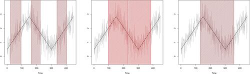
We consider the continuous, piecewise-linear wave2sect signal, defined as the first 450 elements of the wave2 signal from Baranowski, Chen, and Fryzlewicz (2019), contaminated with iid Gaussian noise with $\sigma =0.5$. The signal and a sample path are shown in Figure 2. In this model, we run the NSP procedure, with no overlaps and with the other parameters set as in Section 5.1, (wrongly or correctly) assuming the following, where q denotes the postulated degree of the underlying piecewise polynomial: (a) $q=0$, which wrongly assumes that the true signal is piecewise constant; (b) $q=1$, which assumes the correct degree of the polynomial pieces making up the signal; (c) $q=2$, which over-specifies the degree. We denote the resulting versions of the NSP procedure by NSP ${}_q$ for $q=0,1,2$. The intervals of significance returned by all three NSP ${}_q$ methods are shown in Figure 2. Theorem 2.1 guarantees that the NSP1 intervals each cover a true change-point with probability of at least $1-\alpha =0.9$ and this behavior occurs in this particular realization. The same guarantee holds for the over-specified situation in NSP2, but there is no performance guarantee for NSP0.

Figure 2: Noisy (light grey) and true (black) wave2sect signal, with NSP ${}_q$ significance intervals for $q=0$ (left, misspecified model), $q=1$ (middle, well-specified model), $q=2$ (right, over-specified model). See Section 5.2 for more details.

5.3 Self-Normalized NSP

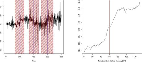
We briefly illustrate the performance of the self-normalized NSP. We define the piecewise-constant squarewave signal as taking the values of 0, 10, 0, 10, each over a stretch of 200 time points. With the random seed set to 1, we contaminate it with a sequence of independent t-distributed random variables with 4 degrees of freedom, with the standard deviation changing linearly from ${\sigma }_1=2\sqrt{2}$ to ${\sigma }_{800}=8\sqrt{2}$. The simulated dataset, showing the “spiky” nature of the noise, is in the left plot of Figure 3.

Figure 3: Left: squarewave signal with heterogeneous $t_4$ noise (black), self-normalized NSP intervals of significance (shaded red), true change-points (blue); see Section 5.3 for details. Right: time series $Q_t$ for $t=1,\dots ,131$. Red: the center of the (single) NSP interval of significance. See Section 6.2 for details.

We run the self-normalized version of NSP with the following parameters: a deterministic equispaced interval sampling grid, $M=1000$, $\alpha =0.1$, $ϵ=0.03$, no overlap; the outcome is in the left plot of Figure 3. Each true change-point is correctly contained within a (separate) NSP interval of significance, and we note that no spurious intervals get detected despite the heavy-tailed and heterogeneous character of the noise.

In addition, we run the self-normalized NSP, with the parameters as above, on heavy-tailed versions of the Noise 300 and Single 300 models from Table 1, in which the Gaussian innovations have been replaced with $t_3$-distributed innovations scaled to have marginal variance 1. For the thus-modified Noise 300 model, self-normalized NSP correctly identifies no intervals of significance in 100 out of 100 simulated sample paths. For the modified Single 300 model, self-normalized NSP correctly identifies one interval of significance in 100/100 simulated sample paths, with the average interval length of 124.54.

6 Data Examples

6.1 The US Ex-post Real Interest Rate

We re-analyze the time series of U.S. ex-post real interest rate (the 3-month treasury bill rate deflated by the CPI inflation rate) considered in Garcia and Perron (1996) and Bai and Perron (2003). The dataset is available at http://qed.econ.queensu.ca/jae/datasets/bai001/. The dataset $Y_t$, shown in the left plot of Figure 4, is quarterly and the range is 1961:1–1986:3, so $t=1,\dots ,T=103$. The arguments outlined in Section 11 of the supplement justify the applicability of NSP in thiscontext.

Figure 4: Left plot: time series $Y_t$; right plot: time series ${\tilde{Y}}_t$; both with piecewise-constant fits (red) and intervals of significance returned by NSP (shaded grey). See Section 6.1 for a detailed description.

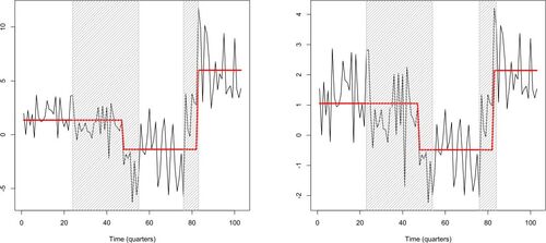
We first perform a naive analysis in which we assume our Scenario 1 (piecewise-constant mean) plus iid $N(0,{\sigma }^2)$ innovations. This is only so we can obtain a rough segmentation which we can then use to adjust for possible heteroscedasticity of the innovations in the next stage. We estimate ${\sigma }^2$ via ${\widehat{\sigma }}_{\text{MAD}}^2$ and run the NSP algorithm with the following parameters: $M=1000$, $\alpha =0.1$, ${\tau }_L={\tau }_R=0$. This returns the set ${\mathcal{S}}_0$ of two significant intervals: ${\mathcal{S}}_0=\{[24,55],[76,83]\}$. We estimate the locations of the change-points within these two intervals via CUSUM fits on $Y_{24:55}$ and $Y_{76:83}$; this returns ${\widehat{\eta }}_1=47$ and ${\widehat{\eta }}_2=82$. The corresponding fit is in the left plot of Figure 4. We then produce an adjusted dataset, in which we divide $Y_{1:47},Y_{48:82},Y_{83:103}$ by the respective estimated standard deviations of these sections of the data. The adjusted dataset ${\tilde{Y}}_t$ is shown in the right plot of Figure 4 and has a visually homoscedastic appearance. NSP run on the adjusted dataset with the same parameters produces the significant interval set ${\tilde{\mathcal{S}}}_0=\{[23,54],[76,84]\}$. CUSUM fits on the corresponding data sections ${\tilde{Y}}_{23:54},{\tilde{Y}}_{76:84}$ produce identical estimated change-point locations ${\tilde{\eta }}_1=47$, ${\tilde{\eta }}_2=82$. The fit is in the right plot of Figure 4.

We could stop here and agree with Garcia and Perron (1996), who also conclude that there are two change-points in this dataset, with locations within our detected intervals of significance. However, we note that the first interval, [23, 54], is relatively long, so one question is whether it could be covering another change-point to the left of ${\tilde{\eta }}_1=47$. To investigate this, we rerun NSP with the same parameters on ${\tilde{Y}}_{1:47}$ but find no intervals of significance (not even with the lower thresholds induced by the shorter sample size $T_1=47$ rather than the original $T=103$). Our lack of evidence for a third change-point contrasts with Bai and Perron’s (2003) preference for a model with three change-points.

However, the fact that the first interval of significance [23, 54] is relatively long could also be pointing to model misspecification. If the change of level over the first portion of the data were gradual rather than abrupt, we could naturally expect longer intervals of significance under the misspecified piecewise-constant model. To investigate this further, we now run NSP on ${\tilde{Y}}_t$ but in Scenario 2, initially in the piecewise-linear model ($q=1$), which leads to one interval of significance: ${\mathcal{S}}_1=\{[57,84]\}$.

This raises the prospect of modeling the mean of ${\tilde{Y}}_{1:57}$ as linear. We produce such a fit, in which in addition the mean of ${\tilde{Y}}_{58:103}$ is modeled as piecewise-constant, with the change-point location ${\tilde{\eta }}_2=79$ found via a CUSUM fit on ${\tilde{Y}}_{58:103}$. We also produce an alternative fit in which the mean of ${\tilde{Y}}_{1:79}$ (up to the change-point) is modeled as linear, and the mean of ${\tilde{Y}}_{80:103}$ (post-change-point) as constant. This is in the right plot of Figure 5 and has a lower BIC value (9.52) than the piecewise-constant fit from the right plot of Figure 4 (10.57). This is because the linear + constant fit uses four parameters, whereas the piecewise-constant fit uses five.

Figure 5: Left plot: $Y_t$ with the quadratic + constant fit; right plot: ${\tilde{Y}}_t$ with the linear + constant fit. See Section 6.1 for a detailed description.

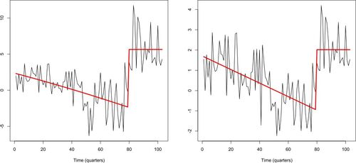
The viability of the linear + constant model for the scaled data ${\tilde{Y}}_t$ is encouraging because it raises the possibility of a model for the original data $Y_t$ in which the mean of $Y_t$ evolves smoothly in the initial part of the data. We construct a simple example of such a model by fitting the best quadratic on $Y_{1:79}$ (resulting in a strictly decreasing, slightly concave fit), followed by a constant on $Y_{80:103}$. The change-point location, 79, is the same as in the linear + constant fit for ${\tilde{Y}}_t$. The fit is in the left plot of Figure 5. It is interesting to see that the quadratic + constant model for $Y_t$ leads to a slightly lower residual variance than the piecewise-constant model (4.9–4.94). Both models use five parameters. We conclude that more general piecewise-polynomial modeling of this dataset can be a viable alternative to the piecewise-constant modeling used in Garcia and Perron (1996) and Bai and Perron (2003). This example shows how NSP, beyond its usual role as an automatic detector of regions of significance, can also serve as a useful tool in achieving improved modelselection.

6.2 House Prices in London Borough of Newham

We consider the average monthly property price $P_t$ in the London Borough of Newham, for all property types, recorded from January 2010 to November 2020 ($T=131$) and accessed on 1st February 2021. The data is available on https://landregistry.data.gov.uk/. We use the logarithmic scale $Q_t=\hspace{0.17em}\log \hspace{0.17em} P_t$ and are interested in the stability of the autoregressive model $Q_t=b+a{Q}_{t-1}+Z_t$. Again, the arguments of Section 11 of the supplement justify the applicability of NSP here.

NSP, run on a deterministic equispaced interval sampling grid, with $M=1000$ and $\alpha =0.1$, with the ${\widehat{\sigma }}_{\text{MOLS}}^2$ estimator of the residual variance (see Section 4 of the supplement) and both with no overlap and with an overlap as defined in formula (3), returns a single interval of significance [24, 96], which corresponds to a likely change-point location between December 2011 and December 2017. Assuming a possible change-point in the middle of this interval, that is, in December 2014, we run two autoregressions (up to December 2014 and from January 2015 onwards) and compare the coefficients. Table 6 shows the estimated regression coefficients (with their standard errors) over the two sections.

Table 6: Parameter estimates (standard error in brackets) in the autoregressive model of Section 6.2.

Parameter	January 2010–December 2014	January 2015–November 2020
b	$-$0.35 (0.2)	0.66 (0.23)
a	1.03 (0.02)	0.95 (0.02)

It appears that both the intercept and the autoregressive parameter change significantly at the change-point. In particular, the change in the autoregressive parameter from 1.03 (standard error 0.02) to 0.95 (0.02) suggest a shift from a unit-root process to a stationary one. This agrees with a visual assessment of the character of the process in the right plot of Figure 3, where it appears that the process is more “trending” before the change-point than it is after, where it exhibits a conceivably stationary behavior, particularly from the middle of 2016 or so. Indeed, the average monthly change in $Q_t$ over the time period January 2010–December 2014 is 0.0061, larger than the corresponding average change of 0.0052 over January 2015–November 2020.

Supplementary Materials

Supplement to the paper in a pdf format; R script to accompany the paper; associated RData file.

Acknowledgments

I wish to thank Yining Chen, Paul Fearnhead, Shakeel Gavioli-Akilagun, Zakhar Kabluchko and David Siegmund for helpful discussions.

Disclosure Statement

There are no competing interests to declare.

Additional information

Funding

Research partially supported by EPSRC grant EP/V053639/1.

References

- Anastasiou, A., and Fryzlewicz, P. (2022), “Detecting Multiple Generalized Change-Points by Isolating Single Ones,” Metrika, 85, 141–174. DOI: 10.1007/s00184-021-00821-6.
- Bai, J., and Perron, P. (1998), “Estimating and Testing Linear Models with Multiple Structural Changes,” Econometrica, 66, 47–78. DOI: 10.2307/2998540.
- Bai, J., and Perron, P. (2003), “Computation and Analysis of Multiple Structural Change Models,” Journal of Applied Econometrics, 18, 1–22. DOI: 10.1002/jae.659.
- Baranowski, R., Chen, Y., and Fryzlewicz, P. (2019), “Narrowest-Over-Threshold Detection of Multiple Change-Points and Change-Point-Like Features,” The Journal of the Royal Statistical Society, Series B, 81, 649–672. DOI: 10.1111/rssb.12322.
- Chan, H. P., and Walther, G. (2013). Detection with the scan and the average likelihood ratio. Statistica Sinica 23, 409–428. DOI: 10.5705/ss.2011.169.
- Chen, Y., Shah, R., and Samworth, R. (2014), “Discussion of ‘Multiscale Change Point Inference’ by Frick, Munk, and Sieling,” Journal of the Royal Statistical Society, Series B, 76, 544–546.
- Cheng, D., He, Z., and Schwartzman, A. (2020), “Multiple Testing of Local Extrema for Detection of Change Points,” Electronic Journal of Statistics, 14, 3705–3729. DOI: 10.1214/20-EJS1751.
- Dette, H., Eckle, T., and Vetter, M. (2020). Multiscale change point detection for dependent data. Scandinavian Journal of Statistics, 47, 1243–1274. DOI: 10.1111/sjos.12465.
- Duy, V. N. L., Toda, H., Sugiyama, R., and Takeuchi, I. (2020), “Computing Valid p-value for Optimal Changepoint by Selective Inference Using Dynaming Programming,” in Advances in Neural Information Processing Systems (Vol. 33), pp. 11356–11367.
- Egorov, V. (1997), “On the Asymptotic Behavior of Self-normalized Sums of Random Variables,” Theory of Probability and Its Applications, 41, 542–548.
- Eichinger, B., and Kirch, C. (2018), “A MOSUM Procedure for the Estimation of Multiple Random Change Points,” Bernoulli, 24, 526–564. DOI: 10.3150/16-BEJ887.
- Fang, X., Li, J., and Siegmund, D. (2020), “Segmentation and Estimation of Change-Point Models: False Positive Control and Confidence Regions,” Annals of Statistics, 48, 1615–1647.
- Fang, X., and Siegmund, D. (2020), “Detection and Estimation of Local Signals,” preprint.
- Frick, K., Munk, A., and Sieling, H. (2014), “Multiscale Change-Point Inference,” (with discussion), Journal of the Royal Statistical Society, Series B, 76, 495–580. DOI: 10.1111/rssb.12047.
- Fryzlewicz, P. (2014), “Wild Binary Segmentation for Multiple Change-Point Detection,” Annals of Statistics, 42, 2243–2281.
- Garcia, R., and Perron, P. (1996), “An Analysis of the Real Interest Rate Under Regime Shifts,” Review of Economics and Statistics, 78, 111–125. DOI: 10.2307/2109851.
- Hao, N., Niu, Y., and Zhang, H. (2013), “Multiple Change-Point Detection via a Screening and Ranking Algorithm,” Statistica Sinica, 23, 1553–1572. DOI: 10.5705/ss.2012.018s.
- Hyun, S., G’Sell, M., and Tibshirani, R. (2018), “Exact Post-Selection Inference for the Generalized Lasso Path,” Electronic Journal of Statistics, 12, 1053–1097. DOI: 10.1214/17-EJS1363.
- Hyun, S., Lin, K., G’Sell, M., and Tibshirani, R. (2021), “Post-Selection Inference for Changepoint Detection Algorithms with Application to Copy Number Variation Data,” Biometrics, 77, 1037–1049. DOI: 10.1111/biom.13422.
- Jewell, S., Fearnhead, P., and Witten, D. (2022), “Testing for a Change in Mean After Changepoint Detection,” Journal of the Royal Statistical Society, Series B, 84, 1082–1104. DOI: 10.1111/rssb.12501.
- Kabluchko, Z. (2007), “Extreme-Value Analysis of Standardized Gaussian Increments,” unpublished.
- Kabluchko, Z., and Wang, Y. (2014), “Limiting Distribution for the Maximal Standardized Increment of a Random Walk,” Stochastic Processes and Their Applications, 124, 2824–2867. DOI: 10.1016/j.spa.2014.03.015.
- Li, H., and Munk, A. (2016), “FDR-control in Multiscale Change-Point Segmentation,” Electronic Journal of Statistics, 10, 918–959. DOI: 10.1214/16-EJS1131.
- Li, H. (2016), “Variational Estimators in Statistical Multiscale Analysis,” PhD thesis, Georg August University of Göttingen.
- Nemirovski, A. (1986), “Nonparametric Estimation of Smooth Regression Functions,” Journal of Computer and System Sciences, 23, 1–11.
- Pein, F., Sieling, H., and Munk, A. (2017), “Heterogeneous Change Point Inference,” Journal of the Royal Statistical Society, Series B, 79, 1207–1227. DOI: 10.1111/rssb.12202.
- Rac˘kauskas, A., and Suquet, C. (2003), “Invariance Principle under Self-normalization for Nonidentically Distributed Random Variables,” Acta Applicandae Mathematicae, 79, 83–103.
- Raimondo, M. (1998), “Minimax Estimation of Sharp Change Points,” Annals of Statistics, 26, 1379–1397.
- Siegmund, D., and Venkatraman, E. S. (1995), “Using the Generalized Likelihood Ratio Statistic for Sequential Detection of a Change-Point,” Annals of Statistics, 23, 255–271.