Poisson-FOCuS: An Efficient Online Method for Detecting Count Bursts with Application to Gamma Ray Burst Detection

Abstract

Gamma ray bursts are flashes of light from distant, new-born black holes. CubeSats that monitor high-energy photons across different energy bands are used to detect these bursts. There is a need for computationally efficient algorithms, able to run using the limited computational resource onboard a CubeSats, that can detect when gamma ray bursts occur. Current algorithms are based on monitoring photon counts across a grid of different sizes of time window. We propose a new method, which extends the recently proposed FOCuS approach for online change detection to Poisson data. Our method is mathematically equivalent to searching over all possible window sizes, but at half the computational cost of the current grid-based methods. We demonstrate the additional power of our approach using simulations and data drawn from the Fermi gamma ray burst monitor archive. Supplementary materials for this article are available online.

Keywords:

• Anomaly detection
• Functional pruning
• Gamma ray bursts
• Page-CUSUM
• Streaming data

1 Introduction

This work is motivated by the challenge of designing an efficient algorithm for detecting gamma ray bursts (GRBs) for CubeSats, such as the HERMES scientific pathfinder mission (Fiore et al. 2020). GRBs are short-lived bursts of gamma ray light caused by the catastrophic accretion of matter into newly formed black holes. Long GRBs are associated with the formation of black holes in the collapse of massive, rapidly rotating stars, whereas short GRBs are associated with coalescence events in neutron star binary systems. These bursts were first detected by satellites in the late 1960s (Klebesadel, Strong, and Olson 1973). At the time of writing there is considerable interest in detecting gamma ray bursts due to their association with gravitational wave events (Luongo and Muccino 2021). For example, during August 17, 2017, the combined detection of the short gamma ray burst GRB170817 and the gravitational wave event GW170817 constrained the source’s location to a region of about 1100 deg², roughly the size of the Ursa Major constellation in the night sky (Abbott et al. 2017). This limited the number of candidate host galaxies to a pool small enough to identify an optical counterpart. A large broadband observation campaign started soon after, leading to insights into many aspects of gravity and astrophysics (Miller 2017).

Instruments detecting GRBs must operate in space, as gamma light wavelengths are absorbed by nitrogen and oxygen in the upper layers of the atmosphere. Because of this, multiple CubeSats missions are being deployed to study them in the coming years (Bloser et al. 2022). CubeSats are compact and therefore relatively cheap to launch into space, but have limited computational power on-board. One of these missions is HERMES (High Energy Rapid Modular Ensemble of Satellites), a mission whose first six units will be launched in near-equatorial orbits during 2023, aiming to build an all-sky monitor for GRBs and other high-energy astronomical transients (Fiore et al. 2020). The HERMES main scientific goal is to monitor the whole sky for GRBs and locate their source directions.

Raw data from a satellite consists of a data stream of photons impacting a detector. The time of a photon impact is recorded in units of microseconds since satellite launch. New photon impacts are recorded on the order of approximately one every 500 microseconds (Campana et al. 2020). A GRB is indicated by a short period of time with an unusually high incidence of photons impacting the detector. Ideally the satellite would detect each GRB, and for each burst it detects it then transmits the associated data to earth.

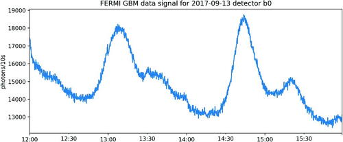
There are a number of statistical challenges associated with detecting GRBs. First, bursts can come from close or far away sources with different intrinsic luminosities, and can therefore be either very bright and obvious to observe or very dim and hard to pick out from other background sources. They can also impact the detector over a variety of timescales. Figure 1 shows two GRBs, one short and intense lasting a fraction of a second, one longer and less intense lasting about 10 sec. These bursts were taken from the FERMI GBM Burst catalogue (Axelsson et al. 2019). Bursts ranging from a fraction of a second to a few minutes are possible (Kumar and Zhang 2015). Second, less than one GRB is recorded per 24 hr on average (Von Kienlin et al. 2020), which is relatively rare in comparison to the velocity of the signal. The background rate at which the satellite detects photons also varies over time. This is due to both rotations of the spacecraft and features of the near-Earth radiation environment at different points in orbit, which leads to irregularly cyclic patterns. This variation is on timescales much larger (many minutes to days) than those on which bursts occur (milliseconds to seconds), and thus is able to be estimated separately from the bursts. Figure 2 gives an example of a background signal.

Fig. 1 Plots of two recorded gamma ray bursts from the FERMI GBM Burst catalogue, with photon counts binned into 0.2 sec and 2 sec intervals.

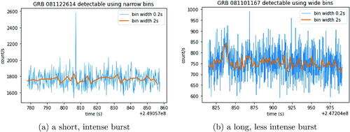
Fig. 2 Example 4 hr of background data from one detector, grouped into 10 sec bins to show background rate fluctuations.

Finally, there are also computational challenges. For example, there is limited computational hardware on board the satellite, and additional constraints may arise due to limitations of the electrical power system and lack of heat dissipation (Fenimore et al. 2003). There is also a substantial computational and energy cost to transmitting data to earth, so only promising data should be sent. This means we require any detection system to have a very low false positive rate.

At a fundamental level, algorithmic techniques for detecting GRBs have gone unchanged through different generations of space-born GRB monitor experiments (Feroci et al. 1997; Paciesas et al. 1999; Fenimore et al. 2003; Meegan et al. 2009). As they reach a detector, high-energy photons are counted over a fundamental time interval and in different energy bands. Count rates are then compared against a background estimate over a number of pre-defined timescales (Li and Ma 1983). To minimize the chance of missing a burst due to a mismatch between the event activity and the length of the tested timescales, multiple different timescales are simultaneously evaluated. Whenever the significance of the excess count is found to exceed a threshold value for that timescale, a trigger is issued.

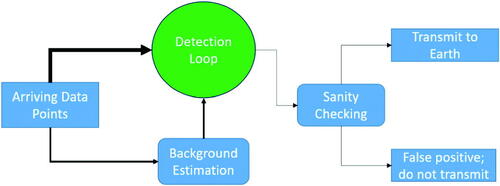
Figure 3 gives a simplified overview of such a detection system. As data arrives we need to both detect whether a gamma ray burst is happening, and update our estimates of the background photon arrival rate. Because of the high computational cost of transmitting data to earth after a detection, if an algorithm detects a potential gamma ray burst there is an additional quality assurance step to determine whether it should be transmitted. This step often includes checking that a gamma ray burst has been detected at two or more detectors on the satellite. The detection algorithm needs to be run at a resolution at which all gamma ray bursts are detectable. By comparison background re-estimation is only required once every second, and the quality assurance algorithm is only needed every time a potential gamma ray burst is detected. Thus, the majority of the computational effort is for the detection algorithm—and how to construct a statistically efficient detection algorithm with low computation is the focus of this article.

Fig. 3 A schematic of the detection system, with the arrow thickness corresponding to the relative velocities of data flows. Most of the computing requirements of the trigger algorithm are within the detection loop, highlighted in green.

As mentioned, current practice for detecting a GRB is to compare observed photon counts with expected counts across a given bin width (Paciesas et al. 2012). However, the choice of bin width affects the ease of discovery of different sizes of burst. Figure 1 shows an example. The short burst in Figure 2(a) is easily detectable with a bin width of 0.2 sec, but lost to smoothing at a 2 sec bin width. In contrast, the burst in Figure 2(b) has a signal too small relative to the noise to be detectable at a 0.2 sec bin width, with the largest observation on the plot being part of the noise rather than the gamma ray burst. Only when smoothed to a bin width of 2 sec does the burst become visually apparent. Therefore, the bin width is first chosen small enough to pick up short bursts, and geometrically spaced windows of size 1, 2, 4, 8,…times the bin width, up to a maximum window size, are run over the data in order to pick up longer bursts.

This article develops an improved approach to detecting GRBs. First we show that using the Page-CUSUM statistic (Page 1954, 1955), and its extension to count data (Lucas 1985) is uniformly better than using a window-based procedure. These schemes require specifying both the pre-change and post-change behavior of the data—in our case, this equates to specifying the background rate of photon arrivals and the rate during the gamma ray burst. While it is reasonable to assume, for our application, that good estimates of the background photon arrival rate are available, specifying the photon arrival rate for the gamma ray burst is difficult due to their heterogeneity in terms of intensity. For detecting changes in mean in Gaussian data, Romano et al. (2023) show how one can implement the sequential scheme of Page (1955) simultaneously for all possible post-change means, and call the resulting algorithm FOCuS. Our detection algorithm involves the nontrivial extension of this approach to the setting of detecting changes in the rate of events for count data. It is based on modeling the arrival of photons on the detector as a Poisson process, and we thus call our detection algorithm Poisson-FOCuS.

Poisson-FOCuS is equivalent to checking windows of any length, with a modified version equivalent to checking windows of any length up to a maximum size. This makes it advantageous for detecting bursts near the chosen statistical threshold whose length is not well described by a geometrically spaced window. In addition, the algorithm we develop has a computational cost lower than the geometric spacing approach, resulting in a uniform improvement on the methods already used for this application with no required tradeoff. These advantages mean that the Poisson-FOCuS algorithm is currently planned to be used as part of the trigger algorithm of the HERMES satellites.

The improvement Poisson-FOCuS achieves over existing windows based methods addresses the aspect of trigger algorithms that has been shown to be most important for increasing power of detecting GRBs. As the computational resource on-board a satellite have increased, trigger algorithms have grown to support an increasing number of criteria, and it has been seen that the most important aspect of any detection procedure is the timescale over which the data is analyzed (McLean et al. 2004). This is in contrast to other possible aspects such as testing data accumulated over multiple, fine-grained energy bands outside the standard 50–300 keV energy band. This did not result in more GRBs being detected by Fermi-GBM, and was eventually turned off to ease the computational burden on the on-board computer (Paciesas et al. 2012).

While early software, such as Compton-BATSE (Gehrels et al. 1993), operated only a few different trigger criteria, a total of 120 are available to the Fermi-GBM (Meegan et al. 2009) and more than 800 to the Swift-BAT (McLean et al. 2004) flight software. Whilst in many cases, this growth in algorithm complexity did not result in additional GRB detection, better coverage of different timescales for GRBs did (Paciesas et al. 2012). During the first four years of Fermi-GBM operations, 135 out of 953 GRBs were detected only over timescales not represented by BATSE algorithms, most of which were over timescales larger than the maximum value tested by BATSE (1.024 sec) (Von Kienlin et al. 2014).

The outline of the article is as follows. In Section 2 we define the mathematical setup of the problem. Section 3 introduces the functional pruning approach, leading to an algorithm and computational implementation specified in Section 4. In Section 5 we give an evaluation of our method on various simulated data, and real data taken from the FERMI catalogue. The article ends with a discussion.

2 Modeling Framework

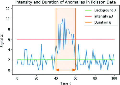
The data we consider take the form of a time-series of arrival times of photons. We can model the generating process for these points as a Poisson process with background parameter $\lambda (t)$, defining anomalies as periods of time which see an increase in the arrival rate over background level. By identifying anomalies, we hope to detect the GRBs that may cause them.

Changes in the background rate, $\lambda (t)$, over time may be due to factors such as the spacecraft’s motion and the orbital radiation environment. They exist on a greater timescale (minutes to days) than the region of time over which a GRB could occur (seconds). We assume that a good estimate of the current background rate $\lambda (t)$ is available. To ease exposition we will first assume this rate is known and constant, and denote it as λ, before generalizing to the nonconstant background rate in Section 4.1. We discuss accounting for error in estimating the background rate in Section 5.2. No autocorrelation is present in our data when this change in background rate has been accounted for, see the supplementary material.

The standard approach to analyzing our data is to choose a small time interval, w, which is smaller than the shortest GRB that we want to detect. Then the data can be summarized by the number of photon arrivals in time bins of length w. We denote the data by $x_1,x_2,\dots ,$ with x_i denoting the number of arrivals in the ith time window. We use the notation $x_{t+1:t+h}=(x_{t+1},\dots ,x_{t+h})$ to denote the vector of observations between the $(t+1)$th and $(t+h)$th time window, and $${\overline{x}}_{t+1:t+h}=\frac{1}{h}\sum _{i=t+1}^{t+h}{x}_i,$$ the mean of these observations. Under our model, if there is no gamma ray burst then each x_i is a realization of X_i , an independent Poisson random variable with parameter λ. If there is a gamma ray burst then the number of photon arrivals will be Poisson distributed with a rate larger than λ. We make the assumption that a gamma ray burst can be characterized by a width, h, and an intensity $\mu >1$ such that if the gamma ray burst starts at time t + 1 then $x_{t+1},\dots ,x_{t+h}$ are realizations of independent Poisson random variables $X_{t+1},\dots ,X_{t+h}$ with mean $\mu \lambda$. See Figure 4 for a visualization of an anomaly simulated directly from this model.

Fig. 4 A simulated example anomaly with intensity multiplier μ = 3 and duration h = 20 against a background λ = 2.

Our algorithm is primarily interested in reducing the computational requirements of constant signal monitoring. Therefore, our model considers a gamma ray burst as a uniform increase in intensity over its length, which does not take into account the unknown shape of a gamma ray burst. If a possible burst is found, an additional round of shape-based sanity checking requiring more computational resources can easily be performed prior to transmission back to Earth.

2.1 Window-based Methods and Detectability

If we assumed we knew the width of the gamma ray burst, h, then detecting it would correspond to testing, for each start time t, between the following two hypotheses:

• ${\mathbf{H}}_0$: $X_{t+1},\dots ,X_{t+h}\sim \text{Poisson}(\lambda )$.

• ${\mathbf{H}}_1$: $X_{t+1},\dots ,X_{t+h}\sim \text{Poisson}(\mu \lambda )$, for some $\mu >1$.

We can perform a likelihood ratio test for this hypothesis. Let $$ denote the log-likelihood for the data $x_{t+1:t+h}$ under our Poisson model with rate $\mu \lambda$. Then the standard (log) likelihood ratio statistic is $$LR=2\left\{{\max }_{\mu >1}\mathcal{l}(x_{t+1:t+h};\mu )-\mathcal{l}(x_{t+1:t+h};1)\right\}.$$

This is 0 if ${\overline{x}}_{t+1:t+h}\le \lambda$, otherwise $$LR=2h\lambda \left\{\frac{{\overline{x}}_{t+1:t+h}}{\lambda }\log \hspace{0.17em}\left(\frac{{\overline{x}}_{t+1:t+h}}{\lambda }\right)-\left(\frac{{\overline{x}}_{t+1:t+h}}{\lambda }-1\right)\right\}.$$

The LR statistic is a function only of the expected count $h\lambda$ and the fitted intensity ${\widehat{\mu }}_{t+1:t+h}:={\overline{x}}_{t+1:t+h}/\lambda$ of the interval $[t+1,t+h]$. Alternatively, it can be written as a function only of the expected count $h\lambda$ and the actual count $h{\overline{x}}_{t+1:t+h}$, which forms the fundamental basis for our algorithm.

In our application, thresholds for gamma ray burst detection are often set based on k-sigma events: values that are as extreme as observing a Gaussian observation that is k standard deviations above its mean. For our one-sided test, the distribution of the likelihood ratio statistic under the null is approximately a mixture of a point mass at 0 and a ${\chi }_1^2$ distribution, each with probability 1/2 (Wilks 1938). We will call a k-sigma event one where the likelihood-ratio statistic exceeds a threshold of k². The definition of a k-sigma event is based on a test for a single anomaly with a specific start and endpoint. In practice, detection of gamma ray bursts is achieved through performing multiple tests, allowing for different start and endpoints of the anomalies. Furthermore, different detection methods may perform more or fewer tests—which can make their statistical performance for the same k-sigma level different. We return to this in Section 5 where we present results that relate the k-sigma level for different methods to average run length, a common measure of Type-I error rate in sequential testing.

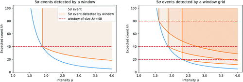
Gamma ray bursts with a combination of high intensity ${\widehat{\mu }}_{t+1:t+h}:=\frac{{\overline{x}}_{t+1:t+h}}{\lambda }$ and long length, as quantified by the expected count $h\lambda$, will have higher associated likelihood ratio statistics and thus be easier to detect. Figure 5 shows regions in this two-dimensional space that correspond to detectable GRBs at different k-sigma levels. Figure 6 shows what happens when we set a fixed threshold and for computational reasons only check intervals of certain lengths. We rely on the fact that a slightly brighter burst will also trigger detection on a longer or shorter interval than optimal. This is the type of approach that current window-based methods take (Paciesas et al. 2012). We can see that, even with a grid of window sizes, we lose detectability if the true width of the GRB does not match one of the window sizes.

Fig. 5 Detectability of GRBs at different k-sigma levels. Shaded regions show values of $h\lambda$ and ${\widehat{\mu }}_{t+1:t+h}$ where the likelihood ratio exceeds k-sigma event thresholds for k = 3 (blue region), k = 5 (orange region) and k = 7 (green region) for a test that uses the correct value of h.

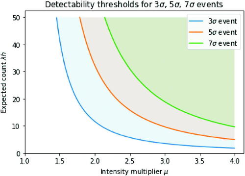
Fig. 6 Detectability of GRBs by the window method, for one window (left) or a grid of three windows (right). The orange shaded area shows the values of $h\lambda$ and ${\widehat{\mu }}_{t+1:t+h}$ where the likelihood ratio exceeds a 5-sigma threshold, and the blue shaded area shows the detectability region form Figure 5. Dashed lines show expected count $h\lambda$ over the window.

2.2 Page-CUSUM for Poisson Data

As a foundation for our detection algorithm, consider the CUSUM (cumulative sum) approach of Page (1955) that was adapted for the Poisson setting by Lucas (1985). These methods can search for gamma ray bursts of unknown width but known size μ, differing from a window method that searches for gamma ray bursts of known width h and unknown size. To run our methods online it is useful to characterize a possible anomaly by its start point τ. We have our hypotheses for the signal at time T:

• ${\mathbf{H}}_0$: There have been no anomalies, that is, $X_1,\dots ,X_T\sim \text{Poisson}(\lambda )$.

• ${\mathbf{H}}_1$: There has been one anomaly, beginning at some unknown time τ, with known intensity multiplier $\mu >1$, that is, $X_1,\dots ,X_{\tau -1}\sim \text{Poisson}(\lambda )$ and $X_{\tau },\dots ,X_T\sim \text{Poisson}(\mu \lambda )$.

Our LR statistic for this test is 0 if ${\overline{x}}_{\tau :T}\le \lambda \frac{\mu -1}{\hspace{0.17em}\log \hspace{0.17em}(\mu )}$ for all τ, otherwise $$LR={\max }_{1\le \tau \le T}\left[2(T-\tau +1)\lambda \left\{\frac{{\overline{x}}_{\tau :T}}{\lambda }\log \hspace{0.17em}\left(\mu \right)-\left(\mu -1\right)\right\}\right].$$

We work with a test statistic, S_T , that is half the likelihood ratio statistic for this test, and compare to a k-sigma threshold of $k^2/2$. S_T can be rewritten in the following form: $$S_T={\left[{\max }_{1\le \tau \le T}\sum _{t=\tau }^T(x_t\hspace{0.17em}\log \hspace{0.17em}(\mu )-\lambda (\mu -1))\right]}^{+},$$ where we use the notation ${[·]}^{+}$ to denote the maximum of the term $·$ and 0. As shown in Lucas (1985), S_T can be updated recursively as $$S_0=0,S_{T+1}={[S_T+x_{T+1}\hspace{0.17em}\log \hspace{0.17em}\mu -\lambda (\mu -1)]}^{+}.$$

It is helpful to compare the detectability of GRBs using S_T with their detectability using a window method. To this end, we introduce the following propositions (see related results in Basseville and Nikiforov 1993; Romano et al. 2023).

Proposition 1.

For some choice of μ against a background rate of λ, let S_T be significant at the k-sigma level. Then there exists some interval $[\tau ,T]$ with associated likelihood ratio statistic that is significant at the k-sigma level.

Proposition 2.

For any k, λ, and h there exists a μ and corresponding test statistic, S_T , that relates directly to a window test of length h, and background rate λ as follows: if, for any t, the data $x_{t+1:t+h}$ is significant at the k-sigma level then $S_{t+h}$ will also be significant at the k-sigma level.

Together these results show that Page’s method is at least as powerful as the window method for detecting a GRB at a fixed k-sigma level. Rather than implementing the window method with a given window size, we can implement Page’s method with the appropriate μ value (as defined by Proposition 2) such that any GRB detected by the window method would be detected by Page’s method. However, Page’s method may detect additional GRBs and these would be detected by the window method with some window size (by Proposition 1). In practice, as shown in Figure 7, Page’s method provides better coverage of the search space.

Fig. 7 Detectability of GRBs by Page-CUSUM for a single μ value (left) and a grid of three μ values (right). Orange shaded area shows the values of $h\lambda$ and ${\widehat{\mu }}_{t+1:t+h}$ where the likelihood ratio exceeds a 5-sigma threshold; the green shaded area shows the detectability region for the corresponding window test as defined by Proposition 2 (left-hand plot); and the blue shaded area shows the detectability region from Figure 5.

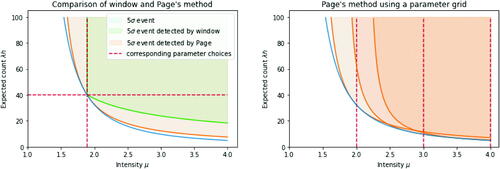
Although the Page-CUSUM approach is more powerful than a window-based approach, to cover the space completely it still requires specifying a grid of values for the intensity of the gamma ray burst. If the actual intensity lies far from our grid values we will lose power at detecting the burst.

3 Functional Pruning

To look for an anomalous excess of count of any intensity and width without having to pick a parameter grid, we consider computing the Page-CUSUM statistic simultaneously for all $\mu \in [1,\infty )$. This can be achieved by considering the test statistic as a function of μ, $S_T(\mu )$. That is, for each T, $S_T(\mu )$ is defined for $\mu \in [1,\infty )$, and for a given μ is equal to the value of the Page-CUSUM statistic for that μ.

By definition, $S_T(\mu )$ is a pointwise maximum of curves representing all possible anomaly start points τ: $$S_T(\mu ):={\left[{\max }_{1\le \tau \le T}\sum _{t=\tau }^T\left[x_t\hspace{0.17em}\log \hspace{0.17em}(\mu )-\lambda (\mu -1)\right]\right]}^{+}.$$

We can view this as $S_T(\mu )={[{\max }_{1\le \tau \le T}{C}_{\tau }^{(T)}(\mu )]}^{+}$, where each curve, $C_{\tau }^{(T)}(\mu )$, corresponds to half the likelihood ratio statistic for a gamma ray burst of intensity μ starting at τ, $$C_{\tau }^{(T)}(\mu ):=\sum _{t=\tau }^T[x_t\hspace{0.17em}\log \hspace{0.17em}(\mu )-\lambda (\mu -1)].$$

Each curve is parameterized by two quantities, as $$C_{\tau }^{(T)}(\mu ):=a_{\tau }^{(T)}\hspace{0.17em}\log \hspace{0.17em}(\mu )-b_{\tau }^{(T)}(\mu -1),$$ where $a_{\tau }^{(T)}={\sum }_{t=\tau }^T{x}_t$ is the actual observed count and $b_{\tau }^{(T)}={\sum }_{t=\tau }^T\lambda =\lambda (T-\tau +1)$ is the expected count on the interval $[\tau ,T]$. As we move from time T to time T + 1 there is a simple recursion to update these coefficients: $a_{\tau }^{(T+1)}=a_{\tau }^{(T)}+x_{T+1},b_{\tau }^{(T+1)}=b_{\tau }^{(T)}+\lambda$. These are linear and do not depend on τ, so the differences between any two curves are preserved with time updates.

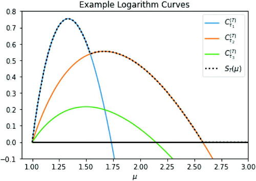
We call $C_{\tau }^{(T)}(\mu )$a logarithmic curve. Figure 8 shows examples of these logarithmic curves. The maximum of $C_{\tau }^{(T)}$ is located at $\mu =a_{\tau }^{(T)}/b_{\tau }^{(T)}$, representing the likelihood ratio for a post-change mean $\mu \lambda ={\overline{x}}_{\tau :T}$. If and only if $a_{\tau }^{(T)}>b_{\tau }^{(T)}$ then the logarithmic curve will be positive for some $\mu >1$. In this case we will define the root of the curve to be the unique ${\mu }^{*}>1$ such that $C_{\tau }^{(T)}({\mu }^{*})=0$.

Fig. 8 Three example logarithmic curves. The statistic $S_T(\mu )$ is defined as the maximum of all logarithmic curves and the 0 line.

3.1 Adding and Pruning Curves

For any two curves $C_{{\tau }_i}^{(T)}$ and $C_{{\tau }_j}^{(T)}$ at a given present time T, we will say that $C_{{\tau }_i}^{(T)}$ dominates $C_{{\tau }_j}^{(T)}$ if $${[C_{{\tau }_i}^{(T)}(\mu )]}^{+}\ge {[C_{{\tau }_j}^{(T)}(\mu )]}^{+},\forall \mu \in [1,\infty ).$$

This is equivalent to saying that there is no value of μ such that the interval $[{\tau }_j,T]$ provides better evidence for an anomaly with intensity μ than $[{\tau }_i,T]$. As the difference between curves is unchanged as we observe more data, this in turn means that for any future point $T_F\ge T$, the interval $[{\tau }_j,T_F]$ will not provide better evidence than $[{\tau }_i,T_F]$. Therefore, the curve associated with τ_j can be pruned, that is, removed from our computational characterization of $S_T(\mu )$.

The following gives necessary and sufficient conditions for one curve to be dominated by another.

Proposition 3.

Let $C_{{\tau }_i}^{(T)}$ and $C_{{\tau }_j}^{(T)}$ be curves that are positive somewhere on $\mu \in [1,\infty )$, where ${\tau }_i<{\tau }_j$ and $C_{{\tau }_i}^{({\tau }_j-1)}$ is also positive somewhere on $\mu \in [1,\infty )$. Then $C_{{\tau }_i}^{(T)}$ dominates $C_{{\tau }_j}^{(T)}$ if and only if $a_{{\tau }_j}^{(T)}/b_{{\tau }_j}^{(T)}\le a_{{\tau }_i}^{({\tau }_j-1)}/b_{{\tau }_i}^{({\tau }_j-1)}$ or equivalently $a_{{\tau }_j}^{(T)}/b_{{\tau }_j}^{(T)}\le a_{{\tau }_i}^{(T)}/b_{{\tau }_i}^{(T)}$. Additionally, it cannot be the case that $C_{{\tau }_j}^{(T)}$ dominates $C_{{\tau }_i}^{(T)}$.

A formal proof is given in the supplementary material, but we see why this result holds by looking at Figure 8. There we see that $C_{{\tau }_i}^{(T)}$ dominates $C_{{\tau }_j}^{(T)}$ precisely when $C_{{\tau }_i}^{(T)}$ has both a greater slope at μ = 1 (which occurs when $C_{{\tau }_i}^{({\tau }_j-1)}$ is positive) and a greater root than $C_{{\tau }_j}^{(T)}$, where (as shown in the proof) the root of a curve $C_{\tau }^{(T)}$ is an increasing function of $a_{\tau }^{(T)}/b_{\tau }^{(T)}$.

4 Algorithm and Theoretical Evaluation

Using Proposition 3 we obtain the Poisson-FOCuS algorithm, described in Algorithm 1. This algorithm stores a list of curves in time order by storing their associated a and b parameters, as well as their times of creation τ, which for the constant λ case can be computed as $T+1-b/\lambda$.

On receiving a new observation at time T, these parameters are updated. If the observed count exceeds the expected count predicted by the most recent curve we also add a new curve which corresponds to a GRB that starts at time T. Otherwise we check to see if we can prune the most recent curve. This pruning step uses Proposition 3, which shows that if any currently stored curve can be pruned, the most recently stored curve will be able to be pruned. (Our pruning check does not does not need to be repeated for additional curves, as on average less than one curve is pruned at each timestep.)

The final part of the algorithm is to find the maximum of each curve, and check if the maximum of these is greater than the threshold. If it is, then we have detected a GRB. The start of the detected GRB is given by the time that the curve with the largest maximum value was added.

Algorithm 1:

Poisson-FOCuS for constant λ

Result: Startpoint, endpoint and test-statistic value for anomaly detected at a k-sigma threshold.

1 set threshold $k^2/2$;

2 initialize empty curve list;

3 while anomaly not yet found do

4 $T\leftarrow T+1$;

5 get actual count X_T ;

6 get expected count λ;//update curves:

7 for curve $$ in curve list

8 $[C_{{\tau }_1}^{(T-1)},\dots ,C_{{\tau }_n}^{(T-1)}]$ do $a_{{\tau }_i}^{(T)}\leftarrow a_{{\tau }_i}^{(T-1)}+X_T$; $b_{{\tau }_i}^{(T)}\leftarrow b_{{\tau }_i}^{(T-1)}+\lambda$;

9 end//add or prune curve:

10 if $X_T/\lambda >\max [a_{{\tau }_n}^{(T)}/b_{{\tau }_n}^{(T)},1]$ then

11 add $C_T^{(T)}:a_T^{(T)}=X_T,b_T^{(T)}=\lambda ,\tau =T$ to curve list;

12 else if $a_{{\tau }_n}^{(T)}/b_{{\tau }_n}^{(T)}<\max [a_{{\tau }_{n-1}}^{(T)}/b_{{\tau }_{n-1}}^{(T)},1]$ then

13 remove $C_{{\tau }_n}^{(T)}$ from curve list;

14 end

//calculate maximum M:

15 for curve $C_{{\tau }_i}^{(T)}$ in curve list do

16 if $\max (C_{{\tau }_i}^{(T)})>M$ then

17 $M\leftarrow \max (C_{{\tau }_i}^{(T)})$;

18 ${\tau }^{*}\leftarrow {\tau }_i$

19 end

20 end

21 if $M>k^2/2$ then

22 anomaly found on interval $[{\tau }^{*},T]$ with $\sqrt{2M}>k$;

23 end

24 end

4.1 Dealing with Varying Background Rate

Algorithm 1 deals with the constant λ case. If $\lambda =\lambda (t)$ is not constant, but an estimate λ_T of $\lambda (T)$ is available at each timestep T, we can apply the same principle but with a change in the definition of $b_{\tau }^{(T)}$. We now have $b_{\tau }^{(T)}:={\sum }_{t=\tau }^T{\lambda }_t$, the total expected count over the interval $[\tau ,T]$. For the algorithm, this only impacts how the coefficients are updated, with the new updates being: $a_{\tau }^{(T+1)}\leftarrow a_{\tau }^{(T)}+X_{T+1},b_{\tau }^{(T+1)}\leftarrow b_{\tau }^{(T)}+{\lambda }_{T+1}$. If we work with a nonhomogeneous Poisson process in this way, it is impossible to recover τ from the coefficients $a_{\tau }^{(T)}$ and $b_{\tau }^{(T)}$, so $C_{\tau }^{(T)}$ must be stored as the triplet $(\tau ,a_{\tau }^{(T)},b_{\tau }^{(T)})$.

The Poisson-FOCuS algorithm gives us an estimate of the start point of a GRB by reporting the interval $[{\tau }^{*},T]$ over which an anomaly is identified. In our application, if the additional sanity checking indicates a GRB is present, the whole signal starting some time before ${\tau }^{*}$ to some time after T is then transmitted from the satellite to Earth. After this has occurred, Poisson-FOCuS can restart immediately provided that a good background rate estimate is available.

4.2 Minimum μ Value

For our application there is an upper limit on the length of a gamma ray burst, and it makes sense to ensure we do not detect gamma ray bursts that are longer than this. To do so, we set an appropriate ${\mu }_{\min }$, and additionally prune curves which only contribute to $S_T(\mu )$ on $1<\mu <{\mu }_{\min }$, by removing, or not adding, curves $C_{\tau }^{(T)}$ to the list if $C_{\tau }^{(T)}({\mu }_{\min })\le 0$, that is $$\frac{a_{\tau }^{(T)}}{b_{\tau }^{(T)}}\le \frac{{\mu }_{\min }-1}{\hspace{0.17em}\log \hspace{0.17em}{\mu }_{\min }}.$$

We can choose ${\mu }_{\min }$ according to our threshold and the maximum expected time period we are interested in searching for bursts over, using the proof of Proposition 2 about detectability for the window-based method, as follows: $${(h\lambda )}_{\max }=\frac{k^2}{2[{\mu }_{\min }\hspace{0.17em}\log \hspace{0.17em}({\mu }_{\min })-({\mu }_{\min }-1)]}.$$

For a 5-sigma threshold, assuming a background rate of one photon every $500\mu$ s, a maximum length of 1 min for a GRB would correspond to ${\mu }_{\min }=1.015$.

4.3 Computational Cost Comparisons

Using a window method, the computational cost per window consists of: adding x_T and λ_T to the window; removing $x_{T-h}$ and ${\lambda }_{t-h}$ from the window; calculating the test statistic and comparing to the threshold. Using Poisson-FOCuS, our computational cost per curve consists of: adding x_T to $a_{\tau }^{(T)}$; adding λ_T to $b_{\tau }^{(T)}$; calculating the maximum of the curve and comparing to the threshold. The computational cost per curve is therefore roughly equal to the computational cost per window. Thus, when evaluating the relative computational cost of Poisson-FOCuS versus a window method we need only calculate the expected number of curves kept by the algorithm at each timestep, and compare against the number of windows used. We now give mathematical bounds on this quantity, as follows:

Proposition 4.

The expected number of curves kept by Poisson-FOCuS without ${\mu }_{\min }$ at each timestep T is $\in [\frac{\hspace{0.17em}\log \hspace{0.17em}(T)}{2},\frac{\hspace{0.17em}\log \hspace{0.17em}(T)+1}{2}]$.

Proposition 5.

The expected number of curves kept by Poisson-FOCuS using some ${\mu }_{\min }>1$ at each timestep is bounded.

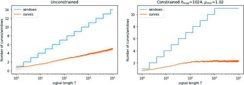
For geometrically spaced windows, over an infinite horizon the number of windows used at each timestep T is $\in [{\hspace{0.17em}\log \hspace{0.17em}}_2(T),{\hspace{0.17em}\log \hspace{0.17em}}_2(T)+1]$, and if a $h_{\max }$ is implemented then this will be bounded after a certain point. Figure 9 gives a comparison of the number of windows and expected number of curves, showing that although the bound from Proposition 5 is difficult to calculate, it is substantially below the corresponding bound on the number of windows. Therefore, Poisson-FOCuS provides the statistical advantages of an exhaustive window search at under half the computational cost of a geometrically spaced one.

Fig. 9 Comparisons of the number of windows and expected number of curves (average over 1000 runs) kept by FOCuS running over a signal with base rate λ = 100 using a 5-sigma threshold, with no constraint on length of GRB (left) and with $h_{\max }=1024$, corresponding to ${\mu }_{\min }=1.02$ (right).

5 Empirical Evaluation

5.1 Simulations of GRBs and Average Run Length Comparison

We have previously worked under the assumption that a threshold level of 5 sigma will be used. In practice, the threshold is a tunable parameter and will be chosen to give a tradeoff between detection sensitivity and number of false detections.

We can make a direct comparison between the sigma threshold and average run length, a standard metric in anomaly detection literature. The average run length is the expected time until we have a false detection if we simulate data under the null hypothesis. This can be calculated for both FOCuS and logarithmically spaced windows, letting us make comparisons between the two by choosing a slightly different sigma threshold based on equal average run lengths. The average run length for each algorithm does not easily translate into an average run length for detecting GRBs, as it does not account for the sanity checking step of the detection algorithm, which can require a GRB to be detected by multiple detectors; nor do the results we present account for any error in estimating the background rate.

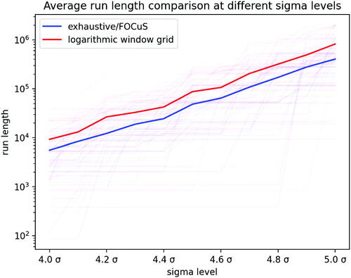
The results are shown in Figure 10. The run length is given in terms of number of observations, so would need to be multiplied by the choice of fundamental bin width, w, to be converted to time. The main message from these results is that for the same average run length we would need to have a threshold that is $0.1\sigma$ higher for FOCuS than for the methods that uses logarithmically spaced windows.

Fig. 10 Comparison between FOCuS and logarithmic window method showing the average run length at different sigma levels.

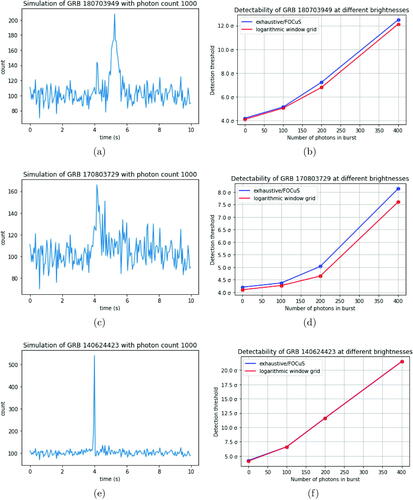
We now compare Poisson-FOCuS with a window based method on synthetic data that has been simulated to mimic known GRBs, but allowing for different intensities of burst. To simulate the data for a chosen known GRB at a range of different brightnesses, the photon stream of the GRB was converted into a random variable via density estimation. One draw from this random variable would give a photon impact time, and n independent draws sorted into time order would give a stream of photon impact times that well approximate the shape of the burst. These were then overlaid on a background photon stream to form a signal that was binned into fundamental time widths of 50ms, which was fed into either Poisson-FOCuS or a geometrically spaced window search. The maximum sigma-level that was recorded when passing over the signal with each method is then plotted for various different brightnesses n. To stabilize any randomness introduced by the use of a random variable for GRB shape, this was repeated 10 times with different random seeds common to both methods and the average sigma-level is plotted.

The extent to which Poisson-FOCuS provides an improvement in detection power depends on the size and shape of the burst, and in particular whether the most promising interval in the burst lines up well with the geometrically spaced window grid. For example, the burst illustrated in Figure 11(c) does not line up with this grid, and Figure 11(d) shows how Poisson-FOCuS provides an improvement in detection power of approximately $0.5\sigma$ for this shape of burst at various different brightnesses, far higher than the approximately $0.1\sigma$ increase in threshold required to give a similar average run length (see Figure 10). However, the shorter burst in Figure 11(e) clearly has a most promising interval of size 1 for this binning choice, which is covered exactly by the logarithmic window grid. Therefore, Poisson-FOCuS provides no improvement over the window grid.

Fig. 11 Plots of runs of FOCuS and window-based method on simulated GRB copies of different brightnesses. Left-hand column shows three example GRBs each simulated to have 1000 photons. Right-hand column shows corresponding largest value of the test statistic as a function of number of photons in GRB. In plot (f) the lines for the two methods almost perfectly overlay one another.

5.2 Bias from Estimating Background Rate

When using Poisson-FOCuS on a dataset requiring background rate estimation, particular care needs to be taken with the choice of the estimator for the background rate. Small, consistent under-estimation of the background rate will be recorded as an anomaly over a long timescale. The ability of any online algorithm to give immediate detections requires a background estimate for time T to be available using only data from $t\le T$, and this can cause challenges with avoiding underestimating the background rate in periods where it is increasing. Furthermore, the presence of a GRB within the data being used to estimate background rate could destabilize the estimation, so robust methods are needed.

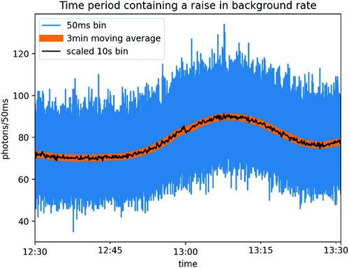
To show this effect, Figure 12 shows a portion of the same data as Figure 2 at a higher resolution. This hour of data was chosen because it contains a smooth rise in background rate, which can give rise to anomalies when using a biased background rate estimation method.

Fig. 12 An hour’s portion of the same data from Figure 2 at higher resolution of 50ms (blue). In black is the data at 10 sec resolution identical to that from Figure 2 but rescaled by 0.005x to fit the graph. In orange is a centered 3 min moving-average background estimate (linewidth increased for visual clarity).

Figure 13 shows the sigma thresholds recorded by Poisson-FOCuS running over this hour’s worth of higher-resolution data using a background estimate of 3 min centered moving-average window (Figure 13(a)), and a 3 min uncentered moving-average window such that background estimates at time T use only data from $t\le T$ (Figure 13(b)). The uncentered method has a large peak in the recorded statistical threshold as it passes over the signal. This is caused by the upward change in background rate, which results in a consistent underestimation of the background rate at time T when using data from just the period prior to T. This bias in background estimation is then interpreted as a very small anomaly over a very long time period.

Fig. 13 Plots of a run of FOCuS over the data using various background estimation methods and parameters: (a) using a unbiased estimator of the background rate; (b) using a biased estimator; (c) using the same biased estimator but with ${\mu }_{\min }=1.1$.

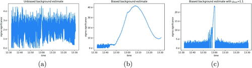
While the effect of a biased background estimation method can be somewhat countered by setting a value for ${\mu }_{\min }>1$ as in Figure 13(c), careful consideration should be given to de-biasing the background estimation method in order to avoid false detections when the background rate is rising (see e.g., Crupi et al. 2023). For example, we show in the next section that reliable detection of GRBs can be obtained using an exponential smoother to estimate the background rate.

5.3 Application to FERMI Data

In the context of HERMES, Poisson-FOCuS is currently being employed for two different purposes. First, a trigger algorithm built using Poisson-FOCuS is being developed for on-board, online GRB detection. To date, a dummy implementation has been developed and preliminary testings performed on the HERMES payload data handling unit computer. Second, Poisson-FOCuS is being employed in a software framework intended to serve as the foundation for the HERMES offline data analysis pipeline (Crupi et al. 2023). In this framework, background reference estimates are provided by a neural network as a function of the satellite’s current location and orientation.

Since no HERMES CubeSats have been launched yet, testing has taken place over Fermi gamma ray burst monitor (GBM) archival data, looking for events which may have evaded the on-board trigger algorithm. The data used for the analysis were drawn from the Fermi GBM daily data, Fermi GBM trigger catalogue, and Ferm GBM untriggered burst candidates catalogue, all of which are publically available at NASA’s High Energy Astrophysics Science Archive Research Center HEASARC (2022a, 2022b), and Bhat (2021).

The algorithm was run over eight days of data, from 00:00:00 2017/10/02 to 23:59:59 2017/10/09 UTC time. This particular time frame was selected because, according to the untriggered GBM Short GRB candidates catalog, it hosts two highly reliable short GRB candidates which defied the Fermi-GBM online trigger algorithm. During this week the Fermi GBM algorithm was triggered by 11 different events. Six of these were classified as GRBs, three as terrestrial gamma ray flashes, one as a local particle event and one as an uncertain event. The Poisson-FOCuS algorithm was run over data streams from 12 sodium iodide GBM detectors in the energy range of 50–300 kiloelectron volts, which is most relevant to GRB detection but excludes the bismuth germanate detectors and higher energy ranges designed to find terrestrial gamma ray flashes.

The data were binned at 100ms. Background count-rates were assessed by exponential smoothing of past observations, excluding the most recent 4 sec, and any curves corresponding to start points older than 4 sec were automatically removed from the curve lists. The returning condition used was the same used by Fermi-GBM: a trigger is issued whenever at least two detectors are simultaneously above threshold. After a trigger, the algorithm was kept idle for 5 min and then restarted.

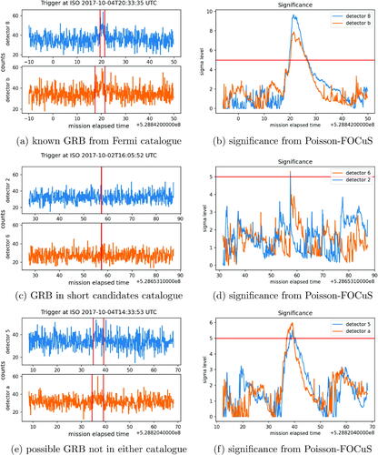
At a 5-sigma threshold, Poisson-FOCuS was able to identify all the six GRBs which also triggered the Fermi-GBM algorithm, one of which is shown in Figure 14(a) and (b). We also observed a trigger compatible with an event in the untriggered GBM Short GRB candidates catalog (Bhat 2021), which is shown in Figure 14(c) and (d). An uncertain event not in either catalogue is shown in Figure 14(e) and (f), which may indicate a GRB that had been missed by earlier searches.

Fig. 14 Three of the triggers found in the FERMI daily data. Left-hand column shows data from the two detectors that give a trigger, and the right-hand column shows the corresponding output from the Poisson-FOCuS algorithm.

6 Discussion

The main purpose of this article was to present a GRB detection algorithm that is mathematically equivalent to searching all possible window lengths, while requiring less computational power than the grid of windows approach. This algorithm is suitable for use on the HERMES satellites, where it has led to a reduction of required computations in a very computationally constrained setting, as well as a simplification of parameter choices by practitioners as values for window lengths in a grid no longer need to be specified.

There is increasing interest in detecting anomalies in other low-compute settings, for example Internet of Things sensors which must continuously monitor a signal (Dey et al. 2018). These may have a limited battery life or limited electricity generation from sensor-mounted solar panels. Therefore, the algorithm we have developed may be of use more widely.

Much of the mathematical work presented in this article is also applicable to the $\mu \in [0,1]$ case that searches for an anomalous lack of count in a signal. When adapting Poisson-FOCuS to this setting, it is important to make sure the algorithm functions well in situations where the counts are small, as these are precisely the locations of anomalies. Combining these two cases would give a general algorithm for detection of anomalies on $\mu \in [0,\infty )$.

Supplementary Materials

Supplementary material contains proofs and empirical results showing the lack of auto-correlation in the GRB data.

Data Availability Statement

Code for Poisson-FOCuS and the analysis for this article is available at the GitHub repository https://github.com/kesward/FOCuS.

Disclosure Statement

No potential conflict of interest was reported by the authors.

Additional information

Funding

This work was supported by the EPSRC grants EP/N031938/1 and EP/R004935/1, and BT as part of the Next Generation Converged Digital Infrastructure (NG-CDI) Prosperity Partnership. We also acknowledge the support of the INAF RSN-5 mini-grant 1.05.12.04.05 “Development of novel algorithms for detecting high-energy transient events in astronomical time series”.

References

- Abbott, B. P., Abbott, R., Abbott, T. D., Acernese, F., Ackley, K., Adams, C., et al. (2017), “Multi-Messenger Observations of a Binary Neutron Star Merger,” The Astrophysical Journal, 848, L12. DOI: 10.3847/2041-8213/aa91c9.
- Axelsson, M., Bissaldi, E., Omodei, N., et al. (2019), “A Decade of Gamma-Ray Bursts Observed by Fermi-LAT: The Second GRB Catalog,” The Astrophysical Journal, 878, 52. DOI: 10.3847/1538-4357/ab1d4e.
- Basseville, M., and Nikiforov, I. V. (1993), Detection of Abrupt Changes: Theory and Application, Englewood Cliffs: Prentice Hall.
- Bhat, N. (2021), “Fermi Gamma-Ray Burst Monitor Untriggered GBM Short GRB Candidates,” available at https://gammaray.nsstc.nasa.gov/gbm/science/sgrb_search.html. Accessed: 2022-05-18.
- Bloser, P. F., Murphy, D., Fiore, F., and Perkins, J. (2022), “Cubesats for Gamma-Ray Astronomy,” arXiv preprint arXiv:2212.11413.
- Campana, R., Fuschino, F., Evangelista, Y., Dilillo, G., and Fiore, F. (2020), “The HERMES-TP/SP Background and Response Simulations,” in Space Telescopes and Instrumentation 2020: Ultraviolet to Gamma Ray (Vol. 11444), pp. 817–824, SPIE. DOI: 10.1117/12.2560365.
- Crupi, R., Fiore, F., et al. (2023), “A Data Driven Framework for Searching Faint Gamma-Ray Bursts,” Unpublished.
- Dey, N., Hassanien, A., Bhatt, C., Ashour, A., and Satapathy, S. (2018), Internet of Things and Big Data Analytics Toward Next-Generation Intelligence, Cham: Springer.
- Fenimore, E., Palmer, D., Galassi, M., Tavenner, T., Barthelmy, S., Gehrels, N., Parsons, A., and Tueller, J. (2003), “The Trigger Algorithm for the Burst Alert Telescope on SWIFT,” AIP Conference Proceedings 662, 491–493.
- Feroci, M., Frontera, F., Costa, E., Fiume, D. D., Amati, L., Bruca, L., et al. (1997), “In-Flight Performances of the BeppoSAX Gamma-Ray Burst Monitor,” in EUV, X-Ray, and Gamma-Ray Instrumentation for Astronomy VIII (Vol. 3114), pp. 186–197, SPIE.
- Fiore, F., Burderi, L., Lavagna, M., Bertacin, R., Evangelista, Y., Campana, R., et al. (2020), “The HERMES-Technologic and Scientific Pathfinder,” in Space Telescopes and Instrumentation 2020: Ultraviolet to Gamma Ray (Vol. 11444), pp. 214–228.
- Fiore, F., et al. (2020), “High Energy Rapid Modular Ensemble of Satellites Scientific Pathfinder,” available at https://www.hermes-sp.eu/. Accessed: 2021-08-03.
- Gehrels, N., Fichtel, C. E., Fishman, G. J., Kurfess, J. D., and Schönfelder, V. (1993), “The Compton Gamma Ray Observatory,” Scientific American, 269, 68–77. DOI: 10.1038/scientificamerican1293-68.
- HEASARC. (2022a), “Fermi GBM Daily Data,” available at https://heasarc.gsfc.nasa.gov/W3Browse/fermi/fermigdays.html. Accessed: 2022-06-07.
- HEASARC. (2022b), “Fermi GBM Trigger Catalog,” available at https://heasarc.gsfc.nasa.gov/W3Browse/fermi/fermigtrig.html. Accessed: 2022-06-07.
- Klebesadel, R. W., Strong, I. B., and Olson, R. A. (1973), “Observations of Gamma-Ray Bursts of Cosmic Origin,” The Astrophysical Journal, 182, L85–L88. DOI: 10.1086/181225.
- Kumar, P., and Zhang, B. (2015), “The Physics of Gamma-Ray Bursts & Relativistic Jets,” Physics Reports, 561, 1–109. DOI: 10.1016/j.physrep.2014.09.008.
- Li, T. P., and Ma, Y. Q. (1983), “Analysis Methods for Results in Gamma-Ray Astronomy,” The Astrophysical Journal, 272, 317–324. DOI: 10.1086/161295.
- Lucas, J. M. (1985), “Counted Data CUSUMs,” Technometrics, 27, 129–144. DOI: 10.1080/00401706.1985.10488030.
- Luongo, O., and Muccino, M. (2021), “A Roadmap to Gamma-Ray Bursts: New Developments and Applications to Cosmology,” Galaxies, 9, 77. DOI: 10.3390/galaxies9040077.
- McLean, K., Fenimore, E. E., Palmer, D., Barthelmy, S., Gehrels, N., Krimm, H., Markwardt, C., and Parsons, A. (2004), “Setting the Triggering Threshold on Swift,” AIP Conference Proceedings, 727, 667–670.
- Meegan, C., Lichti, G., Bhat, P. N., Bissaldi, E., Briggs, M. S., Connaughton, V. (2009), “The Fermi Gamma-Ray Burst Monitor,” The Astrophysical Journal, 702, 791. DOI: 10.1088/0004-637X/702/1/791.
- Miller, M. C. (2017), “A Golden Binary,” Nature, 551, 36–37. DOI: 10.1038/nature24153.
- Paciesas, W. S., Meegan, C. A., Pendleton, G. N., Briggs, M. S., Kouveliotou, C., and Koshut, T. M. et al. (1999), “The Fourth BATSE Gamma-Ray Burst Catalog (revised),” The Astrophysical Journal Supplement Series, 122, 465. DOI: 10.1086/313224.
- Paciesas, W. S., Meegan, C. A., von Kienlin, A., Bhat, P. N., Bissaldi, E., Briggs, M. S., Michael Burgess, J., et al. (2012), “The Fermi GBM Gamma-Ray Burst Catalog: The First Two Years,” The Astrophysical Journal Supplement Series, 199, 18. DOI: 10.1088/0067-0049/199/1/18.
- Page, E. S. (1954), “Continuous Inspection Schemes,” Biometrika, 41, 100–115.
- Page, E. S. (1955), “A Test for a Change in a Parameter Occurring at an Unknown Point,” Biometrika, 42, 523–527.
- Romano, G., Eckley, I. A., Fearnhead, P., and Rigaill, G. (2023), “Fast Online Changepoint Detection via Functional Pruning CUSUM Statistics,” Journal of Machine Learning Research, 24, 1–36. http://jmlr.org/papers/v24/21-1230.html
- Von Kienlin, A., Meegan, C. A., Paciesas, W. S., Bhat, P., Bissaldi, E., Briggs, M. S., Burgess, J. M., Byrne, D. et al. (2014), “The Second Fermi GBM Gamma-Ray Burst Catalog: The First Four Years,” The Astrophysical Journal Supplement Series, 211, 13. DOI: 10.1088/0067-0049/211/1/13.
- Von Kienlin, A., Meegan, C. A., Paciesas, W. S., Bhat, P., Bissaldi, E., Briggs, M. S., et al. (2020), “The Fourth Fermi-GBM Gamma-Ray Burst Catalog: A Decade of Data,” The Astrophysical Journal, 893, 46. DOI: 10.3847/1538-4357/ab7a18.
- Wilks, S. S. (1938), “The Large-Sample Distribution of the Likelihood Ratio for Testing Composite Hypotheses,” The Annals of Mathematical Statistics, 9, 60–62. DOI: 10.1214/aoms/1177732360.