A Tale of Two Datasets: Representativeness and Generalisability of Inference for Samples of Networks

Abstract

The last two decades have seen considerable progress in foundational aspects of statistical network analysis, but the path from theory to application is not straightforward. Two large, heterogeneous samples of small networks of within-household contacts in Belgium were collected using two different but complementary sampling designs: one smaller but with all contacts in each household observed, the other larger and more representative but recording contacts of only one person per household. We wish to combine their strengths to learn the social forces that shape household contact formation and facilitate simulation for prediction of disease spread, while generalising to the population of households in the region. To accomplish this, we describe a flexible framework for specifying multi-network models in the exponential family class and identify the requirements for inference and prediction under this framework to be consistent, identifiable, and generalisable, even when data are incomplete; explore how these requirements may be violated in practice; and develop a suite of quantitative and graphical diagnostics for detecting violations and suggesting improvements to candidate models. We report on the effects of network size, geography, and household roles on household contact patterns (activity, heterogeneity in activity, and triadic closure). Supplementary materials for this article are available online.

KEYWORDS:

• ERGM
• Exponential-family random graph model
• Missing data
• Model-based inference
• Network size
• Regression diagnostics

1 Introduction

Networks of human interaction provide invaluable insights into epidemiology of directly transmitted infectious disease, and there is a great deal of interest in translating network data into epidemic models (Keeling and Eames 2005, for a review). It is common to focus on epidemiologically important settings such as households (Grijalva et al. 2015; Goeyvaerts et al. 2018) and schools (e.g., Mastrandrea, Fournet, and Barrat 2015), and such data are often used as they are for simulating disease spread and evaluating the impact of intervention strategies (e.g., Cencetti et al. 2021). However, observation of larger and broader epidemiologically relevant networks is limited by time, resources, and considerations such as privacy, so it is often indirect or incomplete in a variety of ways, therefore, requiring statistical models to learn network structure from the available data and reconstruct (simulate) networks consistent with it (Krivitsky and Morris 2017).

Exponential-Family Random Graph Models (ERGMs), also called $p^{*}$ models (Wasserman and Pattison 1996; Lusher, Koskinen, and Robins 2012; Schweinberger et al. 2020, among many), are a popular framework for specifying probability models for networks, postulating an exponential family on the sample space of graphs. Most applications of ERG modeling concern a single, completely observed population network, but methods for incomplete or indirect observation exist (Handcock and Gile 2010; Krivitsky and Morris 2017, among others). At the same time, questions of ERGM asymptotics and inference—particularly under varying network size—have been debated in the literature (Schweinberger et al. 2020).

Increasingly, networks are collected in samples, however. Examples include social networks, such as multiple classrooms (Lubbers 2003; Stewart et al. 2019), multiple households (Grijalva et al. 2015; Goeyvaerts et al. 2018), and multiple persons’ social support networks (Ersig, Hadley, and Koehly 2011); but also other types of networks such as connections among brain regions for multiple subjects (Schweinberger et al. 2020, Sec. 8).

Though simpler mathematically, inference from samples of independent, nonoverlapping networks is no less substantively challenging. In practice, the straightforward “iid” inference scenario (e.g., brain networks) is relatively rare, and it is far more common—particularly for social and contact networks—to observe multiple nonoverlapping settings, similar to each other in nature and with the same notion of a relationship, but varying in size, composition, and exogenous influences. This variation is important because size and composition of networks can have profound effects on their structure (Krivitsky et al. 2011). Furthermore, the selection of networks to be observed may itself be a complex process, and the selected networks themselves may be incompletely observed, requiring network model inference to be integrated with survey sampling inference.

Samples of networks also offer new opportunities. With just one network, methods to diagnose how well the model fits—and how well the inference generalises—are limited to working within that network: Hunter, Goodreau, and Handcock (2008a) proposed a form of lack-of-fit testing that compares the observed network’s relational features not explicitly in the model to the distribution of those features simulated from the fitted model, and Koskinen et al. (2018) leveraged missing data techniques to compute an analogue of Cook’s distance for each actor (the effect of observing each actor’s observed relations on parameter estimates). On the other hand, models for independent (if heterogeneous) samples of networks can be diagnosed using familiar techniques developed for regression—provided those techniques can be adapted to networks, including partially observed networks.

A variety of techniques exist for ERG modeling of samples of networks. One popular approach is meta-analysis, pooling individual networks’ estimates (Lubbers 2003). This approach is impractical for large samples of small networks, because the model may be nonidentifiable on each network individually (Vega Yon, Slaughter, and de la Haye 2021). More recent is multilevel (hierarchical) modeling: Zijlstra, Van Duijn, and Snijders (2006) developed it for the related p² model, and Slaughter and Koehly (2016) for a Bayesian ERGM with random effects. Vega Yon, Slaughter, and de la Haye (2021) described exact maximum likelihood inference for samples of very small networks. Also, when modeling a time series of networks, transitions between successive networks are typically treated as conditionally independent (e.g., Leifeld, Cranmer, and Desmarais 2018).

However, assessing an ERGM’s goodness of fit for a sample of networks has tended to be limited to comparing distributions of observed network statistics to expected (e.g., Slaughter and Koehly 2016; Stewart et al. 2019) and replicating diagnostics of Hunter, Goodreau, and Handcock for each network (Vega Yon, Slaughter, and de la Haye 2021). Little attention has been paid to methods appropriate for partially observed networks, for large samples of networks, and to identifying precisely how the model is misspecified.

Here, we consider two samples of within-household contact networks: one more complete but restricted to households with a young child, the other larger and more representative but with only one member’s relations observed in each household, and both heterogeneous in household sizes and compositions. We wish to fit a probability model to these samples to pool their information and combine their strengths, which will allow us to learn about the social forces affecting the formation of their contacts (i.e., inference) and predict their unobserved relations or other households in the population (i.e., prediction and simulation). More generally, we seek to answer three questions:

1. What are we estimating when we jointly fit a model to multiple networks?

2. What do we need to assume to combine information from multiple networks?

3. How do we test these assumptions?

In Section 2, we begin to address Question 1 by describing the household contact datasets and applying the principles of model-based survey sampling inference to make explicit assumptions associated with inference from samples of networks that were previously left implicit. In Section 3, we review ERGM inference for missing data, describe a parameterization for jointly modeling an ensemble of networks, and discuss its inferential properties—and the requirements for valid inference, addressing Question 2. We then consider in Section 4 the different ways in which these requirements may be violated and combine missing data theory with classic generalised linear model (GLM) diagnostics to produce tools for diagnosing lack of fit in the proposed framework, addressing Question 3; and in addition propose fast model selection techniques for ERGMs for ensembles of networks. Finally, in Section 5, we apply these techniques to select and diagnose models for our data, and report our substantive findings.

Additional information can be found in the appendices, referenced throughout. References to appendix figures and tables are prefixed: for example, Figure B5 is in Appendix B.

2 Data and Inferential Questions

2.1 Study Designs

Two paper-based surveys (Goeyvaerts et al. 2018; Hoang et al. 2021) were conducted in Belgium in 2010–2011, using similar survey instruments but differing in sampling design. In both surveys, recruited by random-digit dialing, respondents (or their guardians) reported their and their household members’ demographic information and recorded their contacts over the course of one day, including the contacts’ ages and genders. Approximate duration and frequency of each contact was also recorded, but here, we focus our attention on presence or absence of contacts involving skin-to-skin touching.

The first major difference between the surveys is that whereas in the egocentric (E) survey (Hoang et al. 2021), only one member in each household (the ego) was enrolled; in the other (Goeyvaerts et al. 2018), the whole household (H) was. This within-household sampling design impacts profoundly the information available about the households: while all contacts are known for the networks in the H dataset (Figure 1a), only contacts incident on the one respondent in the household are known for the E dataset (Figure 1b), though, importantly (Krivitsky and Morris 2017), enough information (discussed in Appendix A.1) was collected to identify these contacts uniquely within the household for almost all households.

Fig. 1 Example observation units from the two datasets. Household composition is observed for both, but whereas every contact in the H households is observed, in the E households contacts not involving the ego are missing by design.

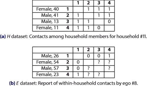
The second major difference is that the H survey was restricted to households with a child aged at most 12, whereas the E survey was not. For convenience, we define E₁₂ to be the set of households in E with at least one such child—that potentially could have been in the H dataset—and $E_{\overline{12}}$ to be those without any, that could not. (Throughout, we will use “presence of a child” and similar wording to refer to this specific criterion.)

More incidentally, the surveys differed slightly in their geographical localization: both surveys included households in the Flemish (Dutch-speaking) areas of Belgium, but only the H survey included households from the (majority-French-speaking) Brussels-Capital region. Also, both surveys’ designs called for fine-grained stratification by age, but the surveyor was not able to adhere to it exactly; and in the H survey, households for which any members’ contacts were not successfully recorded were dropped altogether.

2.2 Descriptive Statistics

After the preprocessing discussed in Appendix A.1, dataset H comprises 317 households of size 2–7 for a total of 1262 members/respondents. Requiring less effort per household to collect, E comprises 1463 respondents whose households (ranging in size 2–8) have a total of 4780 members with 52% of the households’ relationship states observed.

In H, individuals in their mid 20s are underrepresented; E is more representative in this respect, though individuals living alone or in shared housing (disproportionately young adults and seniors) are still excluded. Both datasets’ households are on average gender-balanced, but among E’s respondents women aged 25–55 are overrepresented and adolescents of both genders underrepresented relative to E households’ composition. Most households (H: 71%, E: 75%) were observed on a weekday; 11% of the H households are in Brussels. E₁₂ constitutes 35% of E.

With respect to social structure, the networks are, on average, dense (H: 93%, E₁₂: 90%, $E_{\overline{12}}$: 67%), with H’s networks being more dense on average (vs. E₁₂: $p=0.021$; vs. $E_{\overline{12}}$: $<0.001$), and those of E₁₂ more dense than those of $E_{\overline{12}}$ ($p<0.001$). H’s networks exhibit high triadic closure (global clustering coefficient $\frac{3\times \#\text{triangles}}{\#\text{2-stars}}$ averaging 92%); it cannot be estimated on the partially observed E dataset.

More information can be found in Appendix A.2.

2.3 Implications for Inference

E dataset is representative but consists of egocentric, incomplete networks; H dataset is very selective but of complete networks. E generalises better to the population of Flanders. H allows higher-order (e.g., triadic) effects to be estimated, and includes Brussels. Combining information from multiple surveys with different strengths is not uncommon, and a variety of approaches can be taken (Elliott, Raghunathan, and Schenker 2018).

These data and the substantive problem are particularly amenable to a model-based approach: the ERGM framework seamlessly integrates exogenous (e.g., age) and endogenous (e.g., friend-of-a-friend) effects likely to be relevant. The model-based approach is also feasible: unlike some egocentric data (Krivitsky and Morris 2017) each respondent’s contacts in E could be identified uniquely within the household, so model-based inference of Handcock and Gile (2010) is possible.

For the purposes of prediction (e.g., given the distribution of household compositions, how would an infection brought home from school spread?) we require the analysis to generalise to the population of households in Flanders and Brussels. The missing information principle (Orchard and Woodbury 1972; Breckling et al. 1994) suggests that if the model is accurate enough, it can be generalised to the population despite the heterogeneous and biased sample. More precisely, we require that the sampling process be ignorable or, if viewed as a missing data process, missing at random: the unobserved relationship states must be conditionally independent of the selection process given the model and what is observed (Rubin 1976; Handcock and Gile 2010). In our case, this also means that the model must render the dataset from which the network had come ignorable, which entails accounting for network size, composition, geography, and other relevant effects.

For the purposes of inference (e.g., do mothers have more contact with their children than fathers?), we in addition require consistency and a sampling distribution for our model parameters’ estimators. Fortunately, we can treat these networks as an independent sample: the probability that any member of any of the households in either sample has interacted with a member of one of the other households in either sample is low, and such an interaction is unlikely to affect within-household information in a systematic way in the first place. However, there are further nuances, discussed in Section 4.1.

3 Model Specification and Inference

In modeling an independent sample of networks, we represent two levels of effects: (a) the exogenous and endogenous social forces affecting each network’s relations; and (b) the effects of a network’s exogenous properties such as size, composition, and sampling stratum membership on those social forces. For example, does the presence of a child (a network composition property) affect the contacts between adult men and women in the household (an exogenous relation effect)? Is triadic closure (an endogenous relation effect) stronger or weaker in due to household size (a network property)? We discuss these levels in turn.

3.1 Exponential-Family Random Graph Models for Completely and Partially Observed Networks

We refer the reader to the text book by Lusher, Koskinen, and Robins (2012) and a review by Schweinberger et al. (2020) for detailed discussions of ERGMs’ formulation, interpretation, and inference. For our purposes, let $N=\{1,2,\dots ,n\}$, for $n\ge 2$, be the set of actors whose relations are of interest. Since physical contacts are inherently two-way, we will focus on undirected graphs: the set of potential relations of interest $\mathbb{Y}\subseteq \left\{\right\{i,j\}\in N\times N:i\ne j\}$ is a subset of the set of dyads—distinct unordered pairs of actors. Then, the set of possible graphs of interest $\mathcal{Y}\subseteq 2^{\mathbb{Y}}$ (the set of all possible subsets of $\mathbb{Y}$). We use $\mathit{y}\in \mathcal{Y}$ for the graph data structure, and $y_{i,j}\in \{0,1\}$ as indicator of i and j being connected in $\mathit{y}$ (with $y_{i,j}\equiv y_{j,i}$).

An ERGM is specified by its sample space $\mathcal{Y}$, a collection $\mathit{x}\in \mathcal{X}$ of quantitative and categorical exogenous attributes of actors (e.g., age and gender) or dyads (e.g., distance) used as predictors, and a (sufficient by construction) statistic $\mathit{g}:\mathcal{Y}\times \mathcal{X}\mapsto {\mathbb{R}}^p$. This statistic operationalises the hypothesized social forces affecting the network’s relations. With free model parameters $\mathit{\theta }\in {\mathbb{R}}^p$, a random graph $\mathit{Y}\sim {\text{ERGM}}_{\mathcal{Y},\mathit{x},\mathit{g}}(\mathit{\theta })$ if $${\text{Pr}}_{\mathcal{Y},\mathit{x},\mathit{g}}(\mathit{Y}=\mathit{y};\mathit{\theta })=\hspace{0.17em}\exp \hspace{0.17em}\{\mathit{\theta }·\mathit{g}(\mathit{y},\mathit{x})\}/{\kappa }_{\mathcal{Y},\mathit{x},\mathit{g}}(\mathit{\theta }),\mathit{y}\in \mathcal{Y},$$where ${\kappa }_{\mathcal{Y},\mathit{x},\mathit{g}}(\mathit{\theta })=\sum _{\mathit{y}\prime \in \mathcal{Y}}\hspace{0.17em}\exp \hspace{0.17em}\{\mathit{\theta }·\mathit{g}(\mathit{y}\prime ,\mathit{x})\}$ is the normalizing constant. For the sake of brevity, we will omit specification elements “$\mathcal{Y}$“, “$\mathit{x}$“, “$\mathit{g}$“, and “$\mathit{\theta }$“where unambiguous.

Network statistics that we will use in this work include the edge count $\left|\mathit{y}\right|$ to model propensity to have relations; edge counts within or between exogenous groups of actors to model homophily and other types of mixing; and endogenous effects: count of 2-stars $g_{\text{2-star}}(\mathit{y})={\sum }_{i=1}^n(\begin{array}{c}\left|{\mathit{y}}_i\right|\\ 2\end{array})$ (where $\left|{\mathit{y}}_i\right|$ is the degree—the number of ties incident on actor i) to model degree heterogeneity and count of triangles $g_{\text{triangles}}(\mathit{y})=\sum _{1\le i<j<k\le n}{y}_{i,j}{y}_{j,k}{y}_{k,i}$ to model triadic closure. Ordinarily, we would not use the latter two because of their well-known tendency to induce badly behaved “degenerate” models in large networks and instead use less degeneracy-prone—perhaps curved (Appendix B)—effects (Schweinberger et al. 2020, Sec. 3.1 for context and history). However, this application’s networks are very small and thus largely unaffected, so we use them for their simplicity.

With respect to this ERGM, we may take expectations $\mathbb{E}(·)$ and variances $\mathbb{V}\text{ar}(·)$, including those of the sufficient statistic: let $\mathit{\mu }(\mathit{\theta })\equiv \mathbb{E}\{\mathit{g}(\mathit{Y})\}$ and $\Sigma (\mathit{\theta })\equiv \mathbb{V}\text{ar}\{\mathit{g}(\mathit{Y})\}$.

Given an observed network $\mathit{y}$, an ERGM is typically estimated by maximum likelihood, with $l(\mathit{\theta })\equiv \hspace{0.17em}\log \hspace{0.17em}\text{Pr}(\mathit{Y}=\mathit{y};\mathit{\theta })$ and Fisher information $\mathcal{I}(\mathit{\theta })=-l″(\mathit{\theta })=\Sigma (\mathit{\theta })$. For most interesting models, the normalizing constant $\kappa (\mathit{\theta })$ is intractable, and estimation requires MCMC-based techniques (Schweinberger et al. 2020, Sec. 1.2.1 for references).

If the network is incompletely observed, likelihood estimation proceeds as follows (Handcock and Gile 2010): to the unobserved true population network $\mathit{y}$, an observation process $\text{obs}(·)$ (deterministic or conditioned-on) is applied, producing the observed data structure ${\mathit{y}}^{\text{obs}}\equiv \text{obs}(\mathit{y})$, with $y_{i,j}^{\text{obs}}\in \{0,1,\text{NA}\}$ representing observed-absent, observed-present, and unobserved potential relations, respectively. For the E dataset, $\text{obs}(\mathit{y})$ is such that $$y_{i,j}^{\text{obs}}\equiv \{\begin{array}{cc}{y}_{i,j}\hfill & \text{if }i=1\vee j=1,\hfill \\ \text{NA}\hfill & \text{otherwise}.\hfill \end{array}$$

Let $\mathcal{Y}({\mathit{y}}^{\text{obs}})\equiv \{\mathit{y}\prime \in \mathcal{Y}:\text{obs}(\mathit{y}\prime )={\mathit{y}}^{\text{obs}}\}$: all complete networks that could have produced ${\mathit{y}}^{\text{obs}}$ or, equivalently, all possible imputations of unobserved relations of ${\mathit{y}}^{\text{obs}}$; and define conditional expectation $$\mathit{\mu }(\mathit{\theta }|{\mathit{y}}^{\text{obs}})\equiv \mathbb{E}\{\mathit{g}(\mathit{Y})|\mathit{Y}\in \mathcal{Y}({\mathit{y}}^{\text{obs}})\}$$

and, analogously, conditional covariance $\Sigma (\mathit{\theta }|{\mathit{y}}^{\text{obs}})$. Then, under noninformative sampling and/or missingness at random, the face-value log-likelihood is $l(\mathit{\theta })=\hspace{0.17em}\log \hspace{0.17em}\sum _{\mathit{y}\in \mathcal{Y}({\mathit{y}}^{\text{obs}})}\text{Pr}(\mathit{Y}=\mathit{y};\mathit{\theta })$ and observed information is (Orchard and Woodbury 1972; Sundberg 1974; Handcock and Gile 2010) (1) $${\mathcal{I}}^{\text{obs}}(\mathit{\theta })=\Sigma (\mathit{\theta })-\Sigma (\mathit{\theta }|{\mathit{y}}^{\text{obs}}).$$(1)

Unlike the completely observed case, (1) is not the Fisher information, because it depends on the data ${\mathit{y}}^{\text{obs}}$. The Fisher information, then, also takes the expectation over the possible values of ${\mathit{y}}^{\text{obs}}$ under the model: (2a) $$\mathcal{I}(\mathit{\theta })=\Sigma (\mathit{\theta })-{\mathbb{E}}_{\mathit{Y}}\left[\Sigma \left\{\mathit{\theta }\right|\text{obs}(\mathit{Y})\}\right]$$(2a) (2b) $$=\mathbb{V}{\text{ar}}_{\mathit{Y}}\left[\mathit{\mu }\right\{\mathit{\theta }|\text{obs}(\mathit{Y})\}].$$(2b)

3.2 Multivariate Linear Models for ERGM Parameters

Now, consider a sample of networks indexed $s=1,\dots ,S$, that we wish to model jointly, incorporating network-level effects. There is no unique way to do so; the following approach—drawing on multivariate linear regression models and on seemingly unrelated regression models—has the advantages of familiarity, interpretability, and good inferential properties.

Let ${\mathit{z}}_s\in {\mathbb{R}}^q$ be a row vector of network-level covariates of interest and $\mathit{\beta }\in {\mathbb{R}}^{q\times p}$ the parameter matrix. Set network-level parameters ${\mathit{\theta }}_s\equiv {({\mathit{z}}_s\mathit{\beta })}^{\top }$. Then, jointly, $$({\mathit{Y}}_1,{\mathit{Y}}_2,\dots ,{\mathit{Y}}_S)\sim {\text{ERGM}}_{\mathit{z},\overrightarrow{\mathcal{Y}},\overrightarrow{\mathit{x}},\overrightarrow{\mathit{g}}}(\mathit{\beta })$$if ${\mathit{Y}}_s{\sim }_{\text{ind}}{\text{ERGM}}_{{\mathcal{Y}}_s,{\mathit{x}}_s,{\mathit{g}}_s}({\mathit{\theta }}_s)$. Thus, the components of the network model specification (sample space, sufficient statistic, and any covariates—respectively, ${\mathcal{Y}}_s$ ${\mathit{g}}_s$, and ${\mathit{x}}_s$, collected into S-vectors $\overrightarrow{\mathcal{Y}},\overrightarrow{\mathit{g}}$, $\overrightarrow{\mathit{x}}$) may vary arbitrarily between networks, but their parameter vectors ${\mathit{\theta }}_s$ are parameterized in turn, with elements of $\mathit{\beta }$ determining, in a manner analogous to the linear predictor of a GLM, how network-level covariates affect the ERGM parameters.

Although here we treat q and p as the same for all networks, we show in Appendix E that there is no loss of generality as long as selected elements of $\mathit{\beta }$ can be fixed at 0. Also, this framework can be viewed as a special case (for $\Sigma =\mathbf{0}$) of the model of Slaughter and Koehly (2016), whose prior can be expressed ${\mathit{\theta }}_s{\sim }_{\text{iid}}\text{MVN}\{{({\mathit{z}}_s\mathit{\beta })}^{\top },\Sigma \}$.

Example: Network size effects For a given type of social setting (e.g., classroom, household), bigger networks will typically have lower density ($\left|\mathit{y}\right|/\{n(n-1)/2\}$ for undirected networks), with mean degree ($\left|\mathit{y}\right|/\{n/2\}$) being close to invariant to size. This includes our data (e.g., Figure A2); but the “default” ERGM behavior is to preserve network density (Krivitsky et al. 2011) so that mean degree grows in proportion to n. Krivitsky et al. proposed to adjust this behavior by an offset term of the form $-\hspace{0.17em}\log \hspace{0.17em}(n)\left|\mathit{y}\right|$: other things being equal, the odds of a relation in a network of size n would be scaled by $n^{-1}$, stabilizing the mean degree. But, their result is asymptotic, reliant on sparsity, and only adjusts lower-order properties (density, mixing, and, fortuitously, degree distribution).

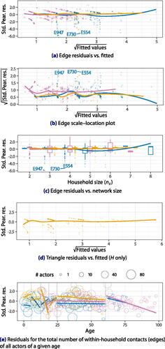
Fig. 2 Selected Pearson residual plots of network statistics for Model 1, modeled after the diagnostic plots produced by R’s (2023) built-in stats package for GLMs. Outliers are identified by their dataset and index within dataset. (Subsets: $H{E}_{12}{E}_{\overline{12}}$)

Butts and Almquist (2015) proposed that the effect of network size on density could be estimated from a sample of networks, with $\hspace{0.17em}\log \hspace{0.17em}(n)$ above multiplied by a free parameter γ, rather than by –1, making the mean degree approximately proportional to $n^{\gamma +1}$. Here, we can accomplish this by setting $z_{s,k}=\hspace{0.17em}\log \hspace{0.17em}(n_s)$ and $g_{s,l}({\mathit{y}}_s)=\left|{\mathit{y}}_s\right|$ for some indices k and l; then $\gamma \equiv {\beta }_{k,l}$. Considering that our networks are small and dense, we can model a nonlinear network size effect by adding a quadratic covariate $z_{s,k+1}={\hspace{0.17em}\log \hspace{0.17em}}^2(n_s)$, with ${\beta }_{k+1,l}$ then becoming its coefficient. (The resulting design matrix is given in Appendix E.) Alternatively, orthogonal polynomial contrasts, a spline, or dummy variables could be used.

3.3 Inference

We now describe this framework’s inferential properties. (Corresponding results for curved ERGMs are given in Appendix B.) Let I_d be an identity matrix of dimension d; let ⊗ be the Kronecker product; and let $Z_s\equiv I_p\otimes {\mathit{z}}_s\in {\mathbb{R}}^{p\times pq}$. Then, we can reexpress ${\mathit{\theta }}_s={\mathit{\beta }}^{\top }{\mathit{z}}_s^{\top }\equiv Z_s\text{vec}(\mathit{\beta })$, for an exponential family with a complete-data likelihood $$\mathcal{L}(\mathit{\beta })=\hspace{0.17em}\exp \hspace{0.17em}\left\{\text{vec}(\mathit{\beta })·\sum _{s=1}^S{Z}_s^{\top }{\mathit{g}}_s({\mathit{y}}_s)\right\}/\prod _{s=1}^S{\kappa }_{{\mathcal{Y}}_s,{\mathit{x}}_s,{\mathit{g}}_s}\left\{{({\mathit{z}}_s\mathit{\beta })}^{\top }\right\}.$$

Let ${\mathit{\mu }}_s(\mathit{\beta }|{\mathit{y}}_s^{\text{obs}})\equiv \mathbb{E}\{{\mathit{g}}_s({\mathit{Y}}_s)|{\mathit{Y}}_s\in \mathcal{Y}({\mathit{y}}_s^{\text{obs}});{({\mathit{z}}_s\mathit{\beta })}^{\top }\}$ and analogously for ${\mathit{\mu }}_s(\mathit{\beta })$, ${\Sigma }_s(\mathit{\beta }|{\mathit{y}}_s^{\text{obs}})$, and ${\Sigma }_s(\mathit{\beta })$. Then, its partially observed Fisher information is $$\mathcal{I}(\text{vec}\mathit{\beta })=\sum _{s=1}^S{Z}_s^{\top }\mathbb{V}{\text{ar}}_{{\mathit{Y}}_s}\left[\mathit{\mu }\right\{\mathit{\beta }|\text{obs}({\mathit{Y}}_s)\}]Z_s.$$

For those networks in the sample that are completely observed, ${\mathit{\mu }}_s(\mathit{\beta }|{\mathit{y}}_s^{\text{obs}})\equiv {\mathit{g}}_s({\mathit{y}}_s)$ and $\mathbb{V}{\text{ar}}_{{\mathit{Y}}_s}[\mathit{\mu }\{\mathit{\beta }|\text{obs}({\mathit{Y}}_s)\}]\equiv {\Sigma }_s(\mathit{\beta })$. Since this is an independent sample of networks, consistency and asymptotic normality of $\widehat{\mathit{\beta }}$ in S can be shown (Sundberg 1974), provided the sampling process is noninformative and $\mathcal{I}(\text{vec}\mathit{\beta })$ is nonsingular asymptotically, which requires the model to be identifiable.

4 Diagnosing Multivariate Linear ERGMs

Whether or not the estimation can be consistent and the inference be generalised to a broader population of households depends on the model being identifiable given available data and on its goodness of fit—both of which must take into account that at least some of the networks in the sample are partially observed. Here, we discuss likely causes and diagnostics for nonidentifiability, develop a generalisation of residual diagnostics to partially observed networks, and consider a variety of ways in which a model may fit the data poorly and how to diagnose this.

4.1 Causes and Diagnostics for Nonidentifiability

The key condition for consistency by Sundberg (1974) is that $\mathcal{I}(\text{vec}\mathit{\beta })$ must be nonsingular. Substantively, there is a number of reasons this condition might not be satisfied.

Nonidentifiable Model Specification

A model may erroneously contain a relationship type or other network feature that is not possible in any potentially sampled network. For a trivial example, counting the number of connections between adults and children is not meaningful in a survey of households without children, nor is counting 2-stars in households of size 2. Similarly, given the large selection of potential network features, and a large selection of potential network-level covariates, it is easy to inadvertently specify a model that is not full-rank. An example of this is network size as a covariate in a sampling process that observes networks of only one distinct size; or a quadratic network size effect if only two distinct sizes are observed. Then the minuend of (2a) (i.e., $\Sigma (\mathit{\beta })$), respectively, has zeros on the diagonal or linear dependence, and the model is not identified even under complete observation.

This form of nonidentifiability can usually be detected during estimation by examining the variance-covariance matrices of simulated sufficient statistics.

Network Observation Process not Informative of the Model

If the sampling process entails partially observed networks, some observation processes may render some otherwise identifiable model specifications nonidentifiable.

Example 1.

Consider an undirected network with actors partitioned into groups A and B. A 3-parameter model whose statistic comprises the counts of all edges, of edges within group A, and of edges between members of A and members of B is identifiable, and its $\Sigma (\mathit{\theta })$ is full-rank. But, if only relationships incident on members of group A (A–A and A–B) are observed, while B–B relations are missing by design, then the elements of $\mathit{\mu }(\mathit{\theta }|{\mathit{y}}^{\text{obs}})$ are affinely dependent, making $\mathcal{I}(\mathit{\theta })$ singular. (See Appendix C.1.)

Example 2.

For an iid sample of S 3-node undirected networks, it is possible to estimate a 3-parameter model with a sufficient statistic comprising edges, 2-stars, and triangles; but not if any one of the three possible relations is unobserved in each network: a direct enumeration of the sample space in Appendix C.2 shows that (2b) is singular.

This form of nonidentifiability is more insidious. Its main symptom is that intermediate estimates of the difference in (2a) are not positive definite; but the algorithm of Handcock and Gile (2010) obtains this difference by subtracting the two simulated variance-covariance matrices, and for data with high missingness fraction and models with many parameters in particular, a false positive can result from Monte Carlo error.

4.2 Residual Diagnostics for Partially Observed Networks

Traditional model diagnostics—whether for linear regression or for ERGMs (Hunter, Goodreau, and Handcock 2008a)—work by comparing the observed data points to those predicted by the fitted model. The approach of Hunter, Goodreau, and Handcock in particular is to simulate networks from the fitted model, and compare the statistics of the simulated networks—particularly those statistics not in the original model—to their observed values. If the observed value falls outside of the range of the simulated, lack of fit is indicated. However, most of the networks in E are partially observed, and this means that there is no “true” observed value for a network feature. We therefore derive equivalent diagnostics for partially observed networks.

For notational convenience, let $\overrightarrow{\mathit{y}}={[{\mathit{y}}_s]}_{s=1}^S$ refer to a vector of completely observed networks. Consider a real-valued function $t(\overrightarrow{\mathit{y}})$ that evaluates a particular network feature of interest, either cumulatively over all of the networks or for a specific network. Analogously to $\mathit{\mu }(·)$ and $\Sigma (·)$ in Section 3.1, let $\tau (\mathit{\beta })\equiv \mathbb{E}\{t(\overrightarrow{\mathit{Y}});\mathit{\beta }\}$ and $\Psi (\mathit{\beta })\equiv \mathbb{V}\text{ar}\{t(\overrightarrow{\mathit{Y}});\mathit{\beta }\}$, and likewise for the conditional expectations.

We can form a standardized (Pearson) residual for $t(\overrightarrow{\mathit{y}})$ by evaluating (3a) $$R_t=\{t(\overrightarrow{\mathit{y}})-\tau (\widehat{\mathit{\beta }})\}/\sqrt{\Psi (\widehat{\mathit{\beta }})},$$(3a) with the expectation and the variance estimated by simulating from the fitted model. Under the true model, this residual would, by construction, have mean 0 and variance close to 1; this also facilitates outlier detection.

If the networks are not completely observed, $t(\overrightarrow{\mathit{y}})$ cannot be evaluated directly, and it is natural to replace it with its empirical best predictor (Hunter et al. 2008b; Stewart et al. 2019; Krivitsky et al. 2023), $$\tau (\widehat{\mathit{\beta }}|{\overrightarrow{\mathit{y}}}^{\text{obs}})\equiv \mathbb{E}\{t(\overrightarrow{\mathit{Y}})|\overrightarrow{\mathit{Y}}\in \mathcal{Y}({\overrightarrow{\mathit{y}}}^{\text{obs}})\},$$where ${\overrightarrow{\mathit{y}}}^{\text{obs}}$ is defined analogously to $\overrightarrow{\mathit{y}}$. Then, (3b) $$R_t=\{\tau (\widehat{\mathit{\beta }}|{\overrightarrow{\mathit{y}}}^{\text{obs}})-\tau (\widehat{\mathit{\beta }})\}/\sqrt{\mathbb{V}{\text{ar}}_{\overrightarrow{\mathit{Y}}}\left[\tau \right\{\widehat{\mathit{\beta }}|\text{obs}(\overrightarrow{\mathit{Y}})\}]}$$(3b)

Estimating the variance in the divisor in (3b) is not trivial. We discuss it in Appendix D.1.

4.3 Causes and Diagnostics for Lack-of-Fit

Within-Network

It may be the case that the within-network model fits poorly. Network statistics used for diagnostics by Hunter, Goodreau, and Handcock (2008a) include the full degree distribution, counts of shared partners (i.e., for a given pair of connected actors, how many common connections do they have?), and the distribution of geodesic distances. All of these can be used as $t(·)$, but it may be impractical for two reasons. First, family networks are relatively small and very dense. This makes the statistics typically used less than informative. Second, the sheer number of networks in the dataset means that diagnosing each network individually is infeasible, but, at the same time, pooling their within-network diagnostics is likely to wash out any effects because of their heterogeneity.

Nonetheless, even if a statistic is suboptimal and difficult to interpret, for a model that fits well, $R_t$ will still have mean 0 and variance close to 1.

Between-Network

It may be the case that the model for the network-level parameters (${\mathit{\theta }}_s$) as a function of global parameters ($\mathit{\beta }$) fits poorly: in particular, it may fail to account for network size and composition effects. At network level, the model has a form similar to that of a GLM. We can thus use the developments of Section 4.2 directly to make familiar diagnostic plots: for some statistic $t_s(\overrightarrow{\mathit{y}})\equiv t({\mathit{y}}_s)$ (e.g., density), we can plot residuals $R_{t_s}$ for $s=1,\dots ,S$ against their respective ${\tau }_s(\widehat{\mathit{\beta }})\equiv \mathbb{E}\{t_s(\overrightarrow{\mathit{Y}})\}$ (the fitted values) or against a candidate predictor $z_{s,\text{new}}$. Or, we can use $\sqrt{\left|R_{t_s}\right|}$ instead for a scale–location plot, analogously to the standard diagnostic plots in R Core Team (2023).

We can also use residuals to test lack-of-fit hypotheses and assess potential explanatory power of $z_{s,\text{new}}$—without the computationally costly ERGM fitting—by regressing $t_s(\overrightarrow{\mathit{y}})-{\tau }_s(\widehat{\mathit{\beta }})$ on $z_{s,\text{new}}$, weighted by their inverse-variance ($\mathbb{V}{\text{ar}}^{-1}\{t_s(\overrightarrow{\mathit{Y}})\}$). Individual networks are independent, so the residuals should be nearly independent as well.

Between-Dataset

If we wish for the fitted model to generalise and render the sampling designs ignorable, the model must account for differences in datasets without incorporating dataset effects directly. This can be done via a hypothesis test, such as a simulation score test, along the lines of that described by Krivitsky (2012) in the context of valued ERGMs, by testing the significance of an explicit dataset effect without refitting the model. Details are given in Appendix D.2.

Nonsystematic Heterogeneity

Lastly, even if there is no systematic bias in the model, there may be between-network heterogeneity due to unobserved factors. The above-described Pearson residuals incidentally provide us with a way to tell whether there is any heterogeneity left to explain: if there is none, $R_{t_s}$ in (3) will, by construction, have mean 0 and variance around 1.

5 Application

We now return to the data we had introduced in Section 2, discuss model specification, and report model diagnostics and results. As one reads this section, it may be helpful to refer to Appendix E for how these effects are represented in the framework described.

We have implemented the methodology described in an extension to the ergm package (Hunter et al. 2008b; Krivitsky et al. 2023) for the R Core Team (2023) statistical environment. To make this methodology accessible to a broad audience, we have published our implementation in an R package, ergm.multi. Materials needed to reproduce the analysis are included in the supplementary file, and the most recent versions of the packages can be found on the Comprehensive R Archive Network (R Core Team 2023) or the Statnet Project software repositories (https://statnet.org).

5.1 Initial Model

A model used to join these two datasets must be substantively meaningful and interpretable. It must account for within-network conditional dependence among the relations. It must make the network size, composition, and dataset effects ignorable to enable generalisable inference. And, it must do so without requiring more information than is available in the data. We therefore dedicate a great deal of attention to formulating and justifying each of the model’s elements.

Here, we develop the initial model, Model 0, which we will then refine using diagnostics.

Household Roles

Our data do not record family relations (e.g., who is married to whom and who is whose child), so we must infer household roles from age and gender. In doing so, there is a tension between interpretability and accuracy: family roles are most conveniently modeled with discrete age categories; but outside of a few critical ages defined exogenously (e.g., school attendance, legal adulthood, and retirement), age effects are likely to be continuous, best modeled semiparametrically (e.g., with splines). Our compromise is to use relatively fine-grained age categories.

A first classification was done according to age: young child (under 6), preadolescent (6–12), adolescent (13–18), young adult (19–24), older adult (25–60), and senior (over 60). (The age cut at 12 was chosen specifically to account for the design boundary.) In order to investigate gender-specific interactions (Goeyvaerts et al. 2018) we subdivided older adults into older female adults and older male adults. A total of seven categories results.

We then modeled mixing by counting the contacts between pairs of these categories—essentially cells of a symmetric 7 × 7 contingency table. Our data about some of these cells are limited, both because some age groups are underrepresented for design reasons discussed above and in Section 2.2, and because some age combinations, such as young children and seniors, are rarely found together in a household (Figure A3 for pairwise counts). Thus, guided by substantive interest, sample size, and design effects, some of the cells were combined for modeling. For example, in modeling contacts with seniors, we combine young children with preadolescents and adolescents with young adults because of their very small sample sizes; but we do not combine all four cells because the combined cell would then cross the age-12 boundary. Similarly, despite a small sample size, young adults with young children were retained as a separate count, because their chances of being parent and child are relatively high. The final parameterization is visualized in Figure 4.

Fig. 3 Estimated effects of network size on conditional odds of an instance of a graph feature. Two-stars and triangles are only possible for $n_s\ge 3$.

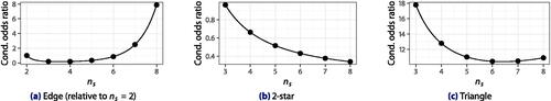
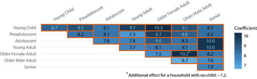
Fig. 4 Parameter estimates for mixing by family role. Borders denote parameterization. Because there is no “intercept” effect in the model, testing them against 0 is not meaningful.

Endogenous Effects

To model actor heterogeneity and triadic closure, we use 2-star and triangle counts, defined in Section 3.1. An additional caveat is that the E dataset, by virtue of only containing relations incident on one individual per household, does not contain information about triadic closure. (See Section 4.1 Example 2 and Appendix C.2.) We thus assume that net of all other effects, the effect of triadic closure on a household of a given size that does not have a child is the same as the effect of triadic closure on a household of that size that does have a child. It is not possible to test this assumption with the available data.

Network Size Effects

The effects of network size on our networks is not trivial: for example, in the analysis of the H dataset by Goeyvaerts et al. (2018), three different density and two different triadic parameters were used, depending on household size. In Model 0, we use the polynomial effects of $\hspace{0.17em}\log \hspace{0.17em}{n}_s$ described in Section 3.2 on edge, 2-star, and triangle counts. This also further guards against ERGM degeneracy, by allowing 2-star and triangle coefficients to decrease with network size.

Other Network-Level Effects

Some of the surveys were conducted on a weekend and others on a weekday (Table A2). Past literature (e.g., Goeyvaerts et al. 2018) suggests that contact patterns may differ depending on the day.

Contact patterns may differ systematically between families that live in detached housing and families that live in apartments. This potential effect has received limited attention in the literature to date. Our data do not include housing type but do include postal codes. The population densities in those postal codes can then be used as a proxy for housing type. We use this potential predictor to illustrate the technique proposed in Section 4.3 of regressing the network-level residuals on potential network-level predictors. Alternatively, we might ask whether or not the post code belongs to any of Belgium’s larger cities.

These properties may be predictive of edge, 2-star, or triangle counts. For the sake of parsimony, Model 0 initially incorporates only weekend effect on density, and diagnostics are used to suggest additional effects.

Design Effects

Last but not least, if we wish to generalise our inference to the population of households, our model must make any design effects ignorable. The substantively motivated effects described above already control for some of those. For example, recall that households in H were omitted if there was nonresponse from even a single member. To the extent that the nonresponse rate is a function of household size (i.e., the bigger the household, the more likely there is at least one nonrespondent), a model that accurately controls for network size will reduce the informativeness of this nonresponse. Similarly, although both surveys’ selection was strongly affected by household members’ ages, particularly children, granular modeling of age mixing effects—particularly for young children and preadolescents—already reduces this design effect’s informativeness.

It is, however, also possible that interactions among adult household members, and other structural features, are affected by a child’s presence—something that Goeyvaerts et al.’s data could not be used to test. We can adjust for this by including the presence of a child in a household as a network-level covariate for density overall, for the endogenous effects, or for mixing. Given the wide range of possibilities, we do not incorporate any such effects into Model 0, instead using residual diagnostics on it to select them.

To account for only the H dataset containing Brussels households, we add an indicator of a Brussels post code as a network-level covariate for density. This completes Model 0.

5.2 Diagnostics

We now apply the techniques from Section 4 to the proposed models. To validate our diagnostic techniques, we also fit a number of reduced models: in Appendix F, we demonstrate how our techniques can identify their deficiencies. In the following, recall our partitioning of E into E₁₂ (at least one child at most 12, potentially in H) and $E_{\overline{12}}$ (no such children).

Effects of a Child in a Household

As discussed, we use diagnostics for Model 0 to select which network features depend on the presence of a child: we calculate the Pearson residuals for counts of edges, 2-stars, triangles, and every pair of actor categories (excluding young children, preadolescents, and seniors), breaking them down by subset H, E₁₂, and $E_{\overline{12}}$. Then, category pairs with extreme residuals that have the same sign for H and E₁₂ but the opposite sign for $E_{\overline{12}}$ may suggest a relevant child effect.

Three mixing cells have residuals with this sign pattern (Table G30): contacts between older female and male adults (H: 2.6, E₁₂: 1.8, $E_{\overline{12}}$: –1.8), two male adults (–1.6, –1.8, 0.6), and two female adults (0.6, 0, –0.1). The latter two are likely spurious and cannot be used in any case due to small sample size (per Appendix A.3).

Adding the effect of absence of a child on the coefficient for contacts between older female and male adults yields Model 1; none of its global or mixing residuals (Table G37) have both the requisite sign pattern and nontrivial magnitude. We focus on Model 1 going forward, but, for illustrative purposes, we also report Model 1a, with the absence-of-child effect on edge count instead.

Additional Substantive Models

As proposed in Section 5.1, we regressed (per Section 4.3) edge, 2-star, and triangle count residuals of Model 1 on a number of candidate predictors, with full results given in Table G34. The linear effect of log-population-density is the most promising ($p=0.046$), yielding Model 2, and, for illustrative purposes, we also report Model 2a, adding the effect of the household being in a major city ($p=0.30$) instead. Specifications for all models are summarized in Table G1, and their complete results and diagnostics are provided in Appendix G.

Table 1 Parameter estimates for Model 1 and Model 2.

Relationship effect	Coefficient (S.E.)
× Network-level effect	Model 1	Model 2
edges × $\hspace{0.17em}\log \hspace{0.17em}(n_s)$	$-14.28{(2.87)}^{\star \star \star }$	$-13.78{(2.98)}^{\star \star \star }$
× ${\hspace{0.17em}\log \hspace{0.17em}}^2(n_s)$	$5.69{(1.29)}^{\star \star \star }$	$5.47{(1.34)}^{\star \star \star }$
if Brussels post code	$0.08(0.19)$	$-0.02(0.20)$
× $\hspace{0.17em}\log \hspace{0.17em}(\text{pop}.\text{dens}.\text{inpostcode})$		$0.04(0.03)$
if on weekend	$0.14{(0.06)}^{\star }$	$0.13{(0.06)}^{\star }$
2-stars	$1.91{(0.78)}^{\star }$	$1.14(0.82)$
× $\hspace{0.17em}\log \hspace{0.17em}(n_s)$	$-2.15{(0.41)}^{\star \star \star }$	$-1.22{(0.44)}^{\star \star }$
× ${\hspace{0.17em}\log \hspace{0.17em}}^2(n_s)$	$0.34{(0.11)}^{\star \star }$	$0.07(0.11)$
triangles	$5.55{(0.97)}^{\star \star \star }$	$7.30{(0.96)}^{\star \star \star }$
× $\hspace{0.17em}\log \hspace{0.17em}(n_s)$	$-3.46{(1.39)}^{\star }$	$-5.65{(1.44)}^{\star \star \star }$
× ${\hspace{0.17em}\log \hspace{0.17em}}^2(n_s)$	$0.93(0.70)$	$1.60{(0.74)}^{\star }$
Young child with young child	$8.60{(1.49)}^{\star \star \star }$	$8.66{(1.54)}^{\star \star \star }$
Young child with preadolescent	$9.10{(1.48)}^{\star \star \star }$	$9.15{(1.54)}^{\star \star \star }$
Preadolescent with preadolescent	$8.17{(1.45)}^{\star \star \star }$	$8.24{(1.51)}^{\star \star \star }$
Adolescent with adolescent	$7.70{(1.43)}^{\star \star \star }$	$7.75{(1.49)}^{\star \star \star }$
Young child with young adult	$9.64{(1.76)}^{\star \star \star }$	$9.67{(1.81)}^{\star \star \star }$
Preadolescent with young adult	$7.25{(1.46)}^{\star \star \star }$	$7.28{(1.51)}^{\star \star \star }$
Adolescent with young adult	$7.73{(1.45)}^{\star \star \star }$	$7.82{(1.51)}^{\star \star \star }$
Young adult with young adult	$7.66{(1.44)}^{\star \star \star }$	$7.70{(1.49)}^{\star \star \star }$
Young child with older female adult	$10.26{(1.45)}^{\star \star \star }$	$10.32{(1.51)}^{\star \star \star }$
Preadolescent with older female adult	$9.67{(1.43)}^{\star \star \star }$	$9.73{(1.49)}^{\star \star \star }$
Adolescent with older female adult	$8.90{(1.43)}^{\star \star \star }$	$8.96{(1.48)}^{\star \star \star }$
Older female adult with older female adult	$7.45{(1.46)}^{\star \star \star }$	$7.50{(1.52)}^{\star \star \star }$
Young child with older male adult	$9.09{(1.43)}^{\star \star \star }$	$9.14{(1.49)}^{\star \star \star }$
Preadolescent with older male adult	$8.76{(1.42)}^{\star \star \star }$	$8.83{(1.48)}^{\star \star \star }$
Adolescent with older male adult	$8.20{(1.42)}^{\star \star \star }$	$8.26{(1.48)}^{\star \star \star }$
Older female adult with older male adult	$10.11{(1.44)}^{\star \star \star }$	$10.17{(1.49)}^{\star \star \star }$
if child absent	$-1.22{(0.30)}^{\star \star \star }$	$-1.20{(0.30)}^{\star \star \star }$
Older male adult with older male adult	$6.59{(1.45)}^{\star \star \star }$	$6.66{(1.50)}^{\star \star \star }$
Older female adult with senior	$8.12{(1.42)}^{\star \star \star }$	$8.20{(1.47)}^{\star \star \star }$
Older male adult with senior	$7.51{(1.45)}^{\star \star \star }$	$7.58{(1.50)}^{\star \star \star }$
Senior with senior	$7.82{(1.40)}^{\star \star \star }$	$7.89{(1.46)}^{\star \star \star }$
Adolescent with young child or preadolescent	$8.07{(1.43)}^{\star \star \star }$	$8.13{(1.48)}^{\star \star \star }$
Young adult with older adult	$8.02{(1.43)}^{\star \star \star }$	$8.07{(1.48)}^{\star \star \star }$
Young child or preadolescent with senior	$8.29{(1.52)}^{\star \star \star }$	$8.34{(1.57)}^{\star \star \star }$
Adolescent or young adult with senior	$9.93{(1.70)}^{\star \star \star }$	$10.01{(1.76)}^{\star \star \star }$
AIC	$3696.6{(0.2)}^{†}$	$3696.8{(0.2)}^{}$
BIC	$3926.9{(0.2)}^{}$	$3933.7{(0.2)}^{}$
log-likehood	$-1813.3{(0.1)}^{}$	$-1812.4{(0.1)}^{}$

Significance: ${}^{\star \star \star }\le 0.001{<}^{\star \star }\le 0.01{<}^{\star }\le 0.05$

${}^{†}$ Standard errors for AIC, BIC, and log-likelihood are due to MCMC error.

Unaccounted-For Between-Dataset Differences

Selected residual plots are provided in Figure 2. We also provide smoothing curves for each subset individually: these curves diverging would indicate that the model had failed to account for some systematic difference between the datasets. Panel (d) (triangle counts) excludes E’s networks, because those contain almost no triadic information.

The network residuals for both edges and triangles (Panels (a)–(d)) are skewed downward and exhibit a striped pattern. This is to be expected regardless of model fit: the underlying network statistics are small counts close to their exogenous upper bounds. There do not appear to be any clear patterns beyond that, and the edge residuals for H, E₁₂, and $E_{\overline{12}}$ coincide on average (Panel (a)). This suggests that the model fuses the two datasets well. The scales of the residuals (Panel (b)) do not exhibit unambiguous patterns either, except for the residuals of $E_{\overline{12}}$ having consistently higher variances than others—whereas the more similar H and E₁₂ networks have similar residual variances.

The dataset hypothesis tests described above and in Appendix D.2 yield p-values 0.068, 0.11, and 0.18 for the edge, the 2-star, and their omnibus test, respectively (with details given in Table G35). Thus, at the conventional significance level, we do not detect unaccounted-for differences between datasets for these features. (In contrast, the respective p-values for Model 0 (Table G28) are 0.019, 0.06, and 0.062, which is more suggestive.)

Outliers

Our residual plots reveal some households inconsistent with typical behavior. For example, the E households #947, #730, and #554 highlighted in Panels (a) and (c) are families of three or four with two older adults (male and female) and a young child (the “respondent”), but no within-household contacts with the child on the day of the survey.

Network Size Effects

Edge residuals against the network size are shown in Panel (c). A model that fails to account for network size would display a linear or curved pattern in the residuals. We see no evidence of such a pattern.

We confirm this with lack-of-fit tests, regressing edge, 2-star, and triangle count residuals on network size treated as categorical (i.e., a dummy variable for each size but one). Lack of fit would be indicated by statistical significance of these regressions; we do not find it for any of the three network statistics (weighted ANOVA omnibus p-vals. 0.20, 0.17, and 0.22, respectively, full results in Table G33).

Nonsystematic Heterogeneity

The standard deviations of Pearson residuals for edges, 2-stars, and triangles are 1.00, 0.99, and 0.98, respectively, all close to 1 as hoped. (Breakdown by data subsets in Table G36.)

Continuous Age Effects

Panel 2e shows the Pearson residuals of the total number of within-household contacts of individuals of each age. We see some indications that discretising ages into categories has an impact. For example, a senior’s propensity to interact appears to drop off as they age, which the cutoff at 60 does not capture. The H household density tends to be slightly underpredicted relative to comparable households in E₁₂, though the differences do not appear to be particularly strong or consistent.

5.3 Results

Model Comparison

Table 1 gives the parameter estimates for Model 1 and Model 2, suggested by our residual diagnostics. (Those for Model 1a and Model 2a are in Tables G38 and G52.) AIC (Table G2) is indifferent between Model 1 ($\text{AIC}=3696.6$) and Model 2 (3696.8) within margin of MCMC error and prefers them over Model 2a (3697.8) and Model 1a (3713.6), the latter only slightly preferred over Model 0 (3714.6). This is as predicted by the residual analyzes discussed in Section 5.2.

A test of population density effect in Model 2 is not significant at conventional level ($\widehat{\beta }=0.04,\mathrm{SE}=0.031,p=0.19$), so we do not find evidence of housing type having an effect—or regional population density is a poor proxy; we leave these questions for future work, except to suggest that type of housing should be considered for future data collection.

Substantive Conclusions

We discuss results primarily from Model 1, though Model 2 yields the same conclusions. Only a few of the effects are interpretable in isolation. In particular, we can conclude with some confidence ($\widehat{\beta }=0.14,\mathrm{SE}=0.056,p=0.015$) that weekends have a positive effect on the number of contacts that are observed in the household, in line with prior literature (Grijalva et al. 2015). Presence of a child in a household is associated with a higher propensity of older male adults and older female adults (likely the parents) to interact with each other (if no child: $\widehat{\beta }=-1.2,\mathrm{SE}=0.30,p<0.001$). We do not detect an effect of being in Brussels on network density ($\widehat{\beta }=0.1,\mathrm{SE}=0.19,p=0.68$).

The estimated polynomial log-network-size effects are shown in Figure 3. Though they are difficult to interpret in isolation from each other, we observe that edge effect counterbalances 2-star and triangle effects, which also decrease with network size, guarding against ERGM degeneracy as hoped. Overall, there is strong evidence that network size effects are present ($p<0.001$), including quadratic ($p<0.001$), and including those on 2-stars and triangles ($p<0.001$). Both 2-star ($p<0.001$) and triangle ($p<0.001$) effects are significant in the presence of others. (Test details are given in Table G32.)

We report the parameter estimates for household member category mixing in a more intuitive layout in Figure 4. Since, unlike Goeyvaerts et al. (2018), we do not use a baseline category (“intercept”), they are not interpretable in isolation but only in contrast with each other. Thus, we conclude that older female adults (i.e., mothers) tend to interact more than older male adults (i.e., fathers) with young children ($\widehat{\Delta }=1.2,\mathrm{SE}=0.47,p=0.013$), preadolescents ($\widehat{\Delta }=0.9,\mathrm{SE}=0.29,p=0.002$), and adolescents ($\widehat{\Delta }=0.7,\mathrm{SE}=0.25,p=0.006$). We thus confirm and expand on similar findings by Goeyvaerts et al. (2018). We also tested whether older female adults interacted with seniors more than older male adults did, whether because they are more likely to care for elderly parents or because in a marriage, the female spouse is typically younger than the male spouse, and there is some evidence for this ($\widehat{\Delta }=0.6,\mathrm{SE}=0.31,\text{one-tailed }p=0.025$). As with housing type, we recommend that future studies record specific familial relations for contacts.

6 Conclusion

Motivated by two collections of networks representing the same phenomena but collected using very different sampling designs, we combined their strengths, facilitating population-wide simulation of household networks. In the process, we identified the requirements of this procedure and developed generally applicable techniques for specifying and diagnosing models for large samples of networks, techniques that, through their relationship to GLMs, can be used by researchers from a wide variety of disciplines. The techniques we have developed do not rely on the networks being completely observed. A user-friendly R implementation is provided.

Our two surveys were conducted in Flanders and Brussels in 2010–2011. It is important to design and analyze household surveys in different settings with different inclusion criteria—but, ideally, compatible measurement instruments—to gain further insights on the contact patterns and the effects of endogenous factors such as triadic closure, exogenous individual attributes such as age, and exogenous household attributes such as size and type of residence. This work provides a foundation for identifying and testing these effects and for confirming the validity of the analysis—and opens the door to design of future cost-effective yet highly informative hybrid network studies.

A number of methodological research directions remain. In our work, we used Pearson residuals. Other types of residuals, such as deviance, tend to be better behaved and could, perhaps, be derived for this family of models. Similarly, Cook’s distance may be possible to compute inexpensively for each network using the approach of Koskinen et al. (2018).

We did not find evidence of nonsystematic heterogeneity of networks. Where such is present, it can be accounted for in a mixed effects framework (Slaughter and Koehly 2016) at an additional computational cost, or perhaps by constructing ERGM sufficient statistics to absorb the variation (Krivitsky 2012; Butts 2017). Alternatively, quasi-likelihood and generalised estimating equation approaches may be extended to samples of networks.

ERGM computational and diagnostic techniques are agnostic to the structure of the sample space, so these approaches directly generalise to directed, temporal, valued, and multilayer network scenarios. For our two surveys in particular, physical contact was not the only relational measurement: the respondents were also asked about the approximate duration of interaction (close proximity) on an ordinal scale (time ranges). Along similar lines, the techniques for calculating standardized residuals under partially observed data may be applicable to other domains that involve modeling independent samples of units which are themselves partially observed.

Supplementary Materials

Appendices A–G:Further details, discussion, and results. (PDF file)

Code and data:Materials to reproduce the analysis. (ZIP file)

Acknowledgments

Krivitsky wishes to thank the UCL Big Data Institute, Elsevier, the University of Wollongong Faculty of Engineering and Information Sciences, and the University of Hasselt for funding travel related to this project, Prof. Raymond Chambers for helpful discussions, Prof. Michael Schweinberger for invaluable feedback on drafts of this article, and the Editor, the Associate Editors, and two anonymous Reviewers, whose comments have led to great improvements to our work.

Disclosure Statement

No potential conflict of interest was reported by the author(s).

Additional information

Funding

This work received funding from the European Research Council (ERC) under the European Union’s Horizon 2020 research and innovation program (PC and NH, grant number 682540—TransMID project, NH grant number 101003688—EpiPose project), from US Army Research Office (PK, award W911NF-21-1-0335 (79034-NS)), and from US National Institutes of Health (PK, award R01 AI138783). Computations were performed on the Katana computing cluster, supported by Research Technology Services at the University of New South Wales.

References

- Breckling, J. U., Chambers, R. L., Dorfman, A. H., Tam, S.-M., and Welsh, A. H. (1994), “Maximum Likelihood Inference from Sample Survey Data,” International Statistical Review, 62, 349–363. DOI: 10.2307/1403766.
- Butts, C. T. (2017), “Baseline Mixture Models for Social Networks.” https://arxiv.org/abs/1710.02773
- Butts, C. T., and Almquist, Z. W. (2015), “A Flexible Parameterization for Baseline Mean Degree in Multiple-Network ERGMs,” The Journal of Mathematical Sociology, 39, 163–167. DOI: 10.1080/0022250X.2014.967851.
- Cencetti, G., Santin, G., Longa, A., Pigani, E., Barrat, A., Cattuto, C., Lehmann, S., Salath’e, M., and Lepri, B. (2021), “Digital Proximity Tracing on Empirical Contact Networks for Pandemic Control,” Nature Communications, 12, 1655. DOI: 10.1038/s41467-021-21809-w.
- Elliott, M. R., Raghunathan, T. E., and Schenker, N. (2018), “Combining Estimates from Multiple Surveys,” in Wiley StatsRef: Statistics Reference Online.
- Ersig, A. L., Hadley, D. W., and Koehly, L. M. (2011), “Understanding Patterns of Health Communication in Families at Risk for Hereditary Nonpolyposis Colorectal Cancer: Examining the Effect of Conclusive versus Indeterminate Genetic Test Results,” Health Communication, 26, 587–594. DOI: 10.1080/10410236.2011.558338.
- Goeyvaerts, N., Santermans, E., Potter, G., Torneri, A., Van Kerckhove, K., Willem, L., Aerts, M., Beutels, P., and Hens, N. (2018), “Household Members Do Not Contact Each Other at Random: Implications for Infectious Disease Modelling,” Proceedings of the Royal Society B: Biological Sciences, 285, 20182201. DOI: 10.1098/rspb.2018.2201.
- Grijalva, C. G., Goeyvaerts, N., Verastegui, H., Edwards, K. M., Gil, A. I., Lanata, C. F., and Hens, N. (2015), “A Household-based Study of Contact Networks Relevant for the Spread of Infectious Diseases in the Highlands of Peru,” PloS One, 10, 1–14. DOI: 10.1371/journal.pone.0118457.
- Handcock, M. S., and Gile, K. J. (2010), “Modeling Social Networks from Sampled Data,” Annals of Applied Statistics, 4, 5–25. DOI: 10.1214/08-AOAS221.
- Hoang, T. V., Coletti, P., Kifle, Y. W., Kerckhove, K. V., Vercruysse, S., Willem, L., Beutels, P., and Hens, N. (2021), “Close Contact Infection Dynamics Over Time: Insights from a Second Large-Scale Social Contact Survey in Flanders, Belgium, in 2010–2011,” BMC Infectious Diseases, 21, 274. DOI: 10.1186/s12879-021-05949-4.
- Hunter, D. R., Goodreau, S. M., and Handcock, M. S. (2008a), “Goodness of Fit for Social Network Models,” Journal of the American Statistical Association, 103, 248–258. DOI: 10.1198/016214507000000446.
- Hunter, D. R., Handcock, M. S., Butts, C. T., Goodreau, S. M., and Morris, M. (2008b), “ergm: A Package to Fit, Simulate and Diagnose Exponential-Family Models for Networks,” Journal of Statistical Software, 24, 1–29. DOI: 10.18637/jss.v024.i03.
- Keeling, M. J., and Eames, K. T. D. (2005), “Networks and Epidemic Models,” Journal of the Royal Society Interface, 2, 295–307. DOI: 10.1098/rsif.2005.0051.
- Koskinen, J., Wang, P., Robins, G., and Pattison, P. (2018), “Outliers and Influential Observations in Exponential Random Graph Models,” 83, 809–830. DOI: 10.1007/s11336-018-9635-8.
- Krivitsky, P. N. (2012), “Exponential-Family Random Graph Models for Valued Networks,” Electronic Journal of Statistics, 6, 1100–1128. DOI: 10.1214/12-EJS696.
- Krivitsky, P. N., Handcock, M. S., and Morris, M. (2011), “Adjusting for Network Size and Composition Effects in Exponential-Family Random Graph Models,” Statistical Methodology, 8, 319–339. DOI: 10.1016/j.stamet.2011.01.005.
- Krivitsky, P. N., Hunter, D. R., Morris, M., and Klumb, C. (2023), “ergm 4: New Features for Analyzing Exponential-Family Random Graph Models,” Journal of Statistical Software, 105, 1–44. DOI: 10.18637/jss.v105.i06.
- Krivitsky, P. N., and Morris, M. (2017), “Inference for Social Network Models from Egocentrically-Sampled Data, with Application to Understanding Persistent Racial Disparities in HIV Prevalence in the US,” Annals of Applied Statistics, 11, 427–455. DOI: 10.1214/16-AOAS1010.
- Leifeld, P., Cranmer, S. J., and Desmarais, B. A. (2018), “Temporal Exponential Random Graph Models with btergm: Estimation and Bootstrap Confidence Intervals,” Journal of Statistical Software, 83, 1–36. DOI: 10.18637/jss.v083.i06.
- Lubbers, M. J. (2003), “Group Composition and Network Structure in School Classes: A Multilevel Application of the p* Model,” Social Networks, 25, 309–332. DOI: 10.1016/S0378-8733(03)00013-3.
- Lusher, D., Koskinen, J., and Robins, G. (2012), Exponential Random Graph Models for Social Networks: Theory, Methods, and Applications, Cambridge: Cambridge University Press.
- Mastrandrea, R., Fournet, J., and Barrat, A. (2015), “Contact Patterns in A High School: A Comparison between Data Collected Using Wearable Sensors, Contact Diaries and Friendship Surveys,” PloS One, 10, e0136497. DOI: 10.1371/journal.pone.0136497.
- Orchard, T., and Woodbury, M. A. (1972), “A Missing Information Principle: Theory and Applications. In: Proceedings of the Sixth Berkeley Symposium on Mathematical Statistics and Probability, Volume 1: Theory of Statistics, pp. 697–715, Berkeley: University of California Press.
- R Core Team (2023), R: A Language and Environment for Statistical Computing, Vienna, Austria: R Foundation for Statistical Computing.
- Rubin, D. B. (1976), “Inference and Missing Data,” Biometrika, 63, 581–592. DOI: 10.1093/biomet/63.3.581.
- Schweinberger, M., Krivitsky, P. N., Butts, C. T., and Stewart, J. R. (2020), “Exponential-Family Models of Random Graphs: Inference in Finite, Super and Infinite Population Scenarios,” Statistical Science, 35, 627–662. DOI: 10.1214/19-STS743.
- Slaughter, A. J., and Koehly, L. M. (2016), “Multilevel Models for Social Networks: Hierarchical Bayesian Approaches to Exponential Random Graph Modeling,” Social Networks, 44, 334–345. DOI: 10.1016/j.socnet.2015.11.002.
- Stewart, J., Schweinberger, M., Bojanowski, M., and Morris, M. (2019), “Multilevel Network Data Facilitate Statistical Inference for Curved ERGMs with Geometrically Weighted Terms,” Social Networks, 59, 98–119. DOI: 10.1016/j.socnet.2018.11.003.
- Sundberg, R. (1974), “Maximum Likelihood Theory for Incomplete Data from an Exponential Family,” Scandinavian Journal of Statistics, 1, 49–58.
- Vega Yon, G. G., Slaughter, A., and de la Haye, K. (2021), “Exponential Random Graph Models for Little Networks,” Social Networks, 64, 225–238. DOI: 10.1016/j.socnet.2020.07.005.
- Wasserman, S. S., and Pattison, P. (1996), “Logit Models and Logistic Regressions for Social Networks: I. An Introduction to Markov Graphs and p*,” Psychometrika, 61, 401–425.
- Zijlstra, B. J. H., Van Duijn, M. A. J., and Snijders, T. A. B. (2006), “The Multilevel p2 Model: A Random Effects Model for the Analysis of Multiple Social Networks,” Methodology, 2, 42–47. DOI: 10.1027/1614-2241.2.1.42.