Using projected cutting planes in the extended cutting plane method

Abstract

In this paper we show that simple projections can improve the algorithmic performance of cutting plane-based optimization methods. Projected cutting planes can, for example, be used as alternatives to standard cutting planes or supporting hyperplanes in the extended cutting plane (ECP) method. In the paper we analyse the properties of such an algorithm and prove that it will converge to a global optimum for smooth and nonsmooth convex mixed integer nonlinear programming problems. Additionally, we show that we are able to solve two old but very difficult facility layout problems (FLP), with previously unknown optimal solutions, to verified global optimum by using projected cutting planes in the algorithm. These solution results are also given in the paper.

Keywords:

• Nonsmooth optimization
• mixed-integer nonlinear programming
• convex nonsmooth functions
• projected cutting planes

2010 Mathematics Subject Classifications:

• 90C11
• 90C25
• 65K05

1. Introduction

A convergence proof for the outer approximation method, able to solve smooth (differentiable) convex mixed integer nonlinear programming (MINLP) problems to an optimal solution, was given in [1]. The paper gave a starting point for a massive number of publications on MINLP applications, new methods and algorithms, many of them for the same class of problems but also some with proven convergence properties for more general classes of MINLP problems. Efforts were, later on, also put on collecting example problems in extensive problem libraries, for example the MINLP Library 2 [2] on which MINLP algorithms and software have been and can be evaluated. Several overviews and performance studies on state of the art algorithms and software for MINLP problems have also been published [3,4].

In this paper we will analyse a modified version of one of these methods, the extended cutting plane (ECP) method [5], which has its origin in the method of Kelley [6] from 1960. In Kelley's method cutting planes are used to overestimate the feasible region and make the relaxation tighter in order to solve smooth convex nonlinear programming (NLP) problems to an optimal solution by a sequence of linear programming (LP) problems. The method was extended to smooth convex MINLP problems in [5] where a convergence proof for the extended cutting plane (ECP) method was given. In a series of papers the ECP method has been further extended to smooth pseudoconvex MINLP problems in [7,8] and nonsmooth convex MINLP problems in [9]. The method was further proven to solve generalized convex MINLP problems using cutting planes and supporting hyperplanes to a global optimal solution in [10–12]. Note that Horst and Tuy [13] have considered nonsmooth problems with linear outer approximations similar to cutting planes and supporting hyperplanes, as well. Standard cutting planes and supporting hyperplanes can also be replaced by (or used together with) projected cutting planes in the ECP algorithm [14]. A projected cutting plane is a cutting plane generated at a MILP solution point or at the projected point. The projected point is obtained by projecting the MILP solution to the kernel of the linearization of the most violated constraint at the MILP solution point. This procedure can be continued to find different projected points. Similar projections has been used in the projection method [15] to find a feasible point from the intersection of convex sets. In [16,17] it is shown that the projection method converges to a feasible point. In [18] certain projections in nonsmooth NLP optimization was considered, as well. In this paper we consider more closely the convergence properties of the algorithm when projected cutting planes based on repeated projection steps are used to solve smooth and nonsmooth convex MINLP problems.

In Kelley's method a sequence of LP problems are solved to obtain points where cuts are to be generated. As LP problems in Kelley's method are replaced by MILP problems in the ECP method, the computational load is, generally, much heavier in the mixed integer case. However, cuts need not be generated at optimal solution points of the MILP subproblems. In proving that the solution sequence of the MILP subproblems converges to a global optimum of the MINLP problem, only the final MILP subproblem needs to be solved to optimality. When considering the ECP method, this observation is very essential since solving a single MILP problem to optimality, by a branch and bound method, may require solving millions of LP subproblems. This issue was discussed in [8], where it was shown that the efficiency of the ECP method can be clearly improved when the cuts are generated mainly at integer feasible and not only at optimal MILP solution points. Such a procedure is easily implementable in an algorithm solving MILP subproblems with solvers like CPLEX [19] or Gurobi [20]. In these solvers the solution procedure can be interrupted after an integer feasible solution has been found and the procedure can therafter be continued utilizing the whole old branch and bound tree. In the ECP procedure, as described in [8], the above property was utilized by using the ‘mip solutions limit’ (msl) parameter, when solving the MILP subproblems. After each iteration, either new cuts are added or the mip solutions limit is increased.

Since the MILP subproblem solutions are integer feasible it should be noted that two distinct sequences of points are obtained wherefrom upper and a lower bounds on the objective function can be calculated. Integer feasible MILP points being feasible in the MINLP problem give upper bounds while optimal MILP points being infeasible in the MINLP problem give lower bounds (assuming the objective function is minimized). Termination of the algorithm occurs when the gap between the bounds is closed or is small enough. In case all MILP subproblems are solved to optimality only one sequence of underestimating lower bounds of the objective function is obtained and an ε-termination criteria on the most violating constraint function is used.

A notable property of the algorithm is also that cuts are generated at integer feasible points. This is sometimes an advantage since there exist applied problems where nonlinear functions are not evaluatable at real values on integer variables [21]. This property does, however, not generally retain when cuts are replaced by supporting hyperplanes. Supports are generated on the boundary of the relaxed feasible region. In addition to an (integer feasible) MILP point, being infeasible in the MINLP problem, a feasible MINLP point and a line search is usually needed to obtain a point on the boundary of the relaxed feasible region of the MINLP problem, where a supporting hyperplane is generated. When projected cuts are used, we will later show, that it is still possible to retain the same property for projected cuts as for standard ones, i.e. that the projected points may remain integer feasible.

When comparing cuts and supporting hyperplanes, one advantage of a supporting hyperplane is that it, generally, results in a tighter relaxation of a specific constraint, than a standard cutting plane. On the other hand, cutting planes are easier to calculate and several cuts (i.e. for different constraints) can be generated at the same MILP solution, while a point on the boundary of the feasible region of the MINLP problem rarely is valid to generate supports for several constraints. A higher number of cuts gives a tighter relaxation of the entire feasible region of the MINLP problem, resulting, often, in that fewer subproblems need be solved to obtain the optimal solution of the MINLP problem. On the other hand, a higher number of cuts, usually, also reduces the computational efficiency to solve the MILP subproblems and although fewer subproblems need be solved, the computational load to solve the entire MINLP problem may be higher.

Projected cutting planes have, in principle, the same advantages as standard cutting planes when comparing them to supporting hyperplanes. However, a projected cutting plane has an advantage when comparing it to a standard cutting plane. A projection moves the infeasible point towards the boundary of the feasible region and makes the projected cutting plane tighter. If a projection would move the point exactly to the boundary, then a projected cut would be a supporting hyperplane at this point. This is, however, not always desirable as the number of supports, that can be generated at a point on the boundary, is generally lower than the number of cuts that can be generated at a point in the infeasible region of the MINLP problem. It should also be mentioned that while a projection moves a point closer to the boundary of the feasible region it is not always possible to reach the boundary if some or all integer variables are fixed in the projection. This can, though, be avoided when relaxed values are allowed also for integer variables.

We will in the following show how projected points are calculated. The procedure can be applied in several steps, reprojecting already calculated projected points. In this case gradients or subgradients of the considered constraint need be calculated in every step of the reprojection. This issue and the convergence properties of the algorithm are considered in the next sections. In the final numerical section we will illustrate the computational procedure first using a simple example. Thereafter, we show that we were able to solve some very difficult facility layout problems (FLP), with formerly unknown optimal solutions, to verified global optimal solutions when using projected cutting planes instead of standard cutting planes in the ECP algorithm.

2. The MINLP problem

The MINLP problem to be solved is formulated as follows, (P) $\begin{array}{rl}& {\mathbf{x}}^{\ast }\in {\mathrm{a}\mathrm{r}\mathrm{g}\mathrm{m}\mathrm{i}\mathrm{n}}_{\mathit{x}\in L\cap C\cap Y}{\mathbf{c}}^T\mathbf{x}\\ & L=\{\mathbf{x}\in X\mid \mathbf{A}\mathbf{x}\le \mathbf{a}\}\\ & C=\{\mathbf{x}\in X\mid \mathbf{g}(\mathbf{x})\le \mathbf{0}\}\\ & Y=\{\mathbf{x}\in X\mid x_i\in \mathbb{Z},i\in I_{\mathbb{Z}},|I_{\mathbb{Z}}|\le n\}\\ & X=\{\mathbf{x}\in {\mathbb{R}}^n\mid {\mathbf{x}}_L\le \mathbf{x}\le {\mathbf{x}}_H\}\end{array}$(P) i.e. find a vector ${\mathbf{x}}^{\ast }$ of bounded real and integer variables, minimizing a linear function ${\mathbf{c}}^T\mathbf{x}$ in $L\cap C\cap Y$. The continuous relaxation $L\cap C$ of $L\cap C\cap Y$ is supposed to be convex. We assume there exists an optimal solution ${\mathbf{x}}^{\ast }$ and that the relaxed exterior L\C is nonempty and in case supporting hyperplanes (needing a line search procedure) are used that the relaxed interior $\{\mathbf{x}\in L\mid \mathbf{g}(\mathbf{x})<\mathbf{0}\}$ is nonempty as well. The sets L and C are defined by linear and nonlinear inequality constraints, respectively. The integer variables in $\mathbf{x}$ are defined by the index set $I_{\mathbb{Z}}$ in Y and the bounds of all variables are defined in X. The nonlinear constraint functions $\mathbf{g}$ in C are in this paper assumed to be convex, smooth or nonsmooth. If a smooth or nonsmooth convex objective function f is to be minimized an additional variable $x_{n+1}$ can be minimized and the objective function be written as an additive constraint in C, as $f\left(\mathbf{x}\right)-x_{n+1}\le 0$. If the objective function would be a convex quadratic function $f\left(\mathbf{x}\right)={\mathbf{x}}^T\mathbf{Q}\mathbf{x}$ then it can replace the linear objective function ${\mathbf{c}}^T\mathbf{x}$ in case the MILP subsolver in the ECP algorithm, is replaced by a MIQP subsolver. This can be done, for example, using the MILP/MIQP solvers in CPLEX and Gurobi.

3. Supporting hyperplanes, standard cutting planes or projected cutting planes

In a recent paper of Serrano et al. [22] it was shown that the supporting hyperplane algorithm [23] is equivalent to Kelley's cutting plane algorithm when reformulating the feasible region of the problem using its (sublinear) gauge function. This is theoretically interesting and in principle the case (neclecting the numerical differences) when comparing the smooth convex NLP algorithms of Kelley [6] and Veinott [24]. This also applies in the mixed integer case when considering the equivalence between the extended cutting plane method for smooth convex MINLP problems in Westerlund and Pettersson [5] and the supporting hyperplane method for smooth convex MINLP problems in Kronqvist et al. [23].

Supporting hyperplanes are halfspaces in the same way as cutting planes, cutting off a part of the infeasible region of a convex MINLP problem, while no part of the feasible region of the problem is cut off. A cutting plane has the property that it cuts off the MILP solution point where it is generated, as well. This is obvious as standard cutting planes are generated at points in the infeasible region of the MINLP problem. A supporting hyperplane is, on the other hand, generated at a point on the boundary of the feasible region (of the MINLP problem). It is, thus, obvious that such a point should not be cut off. To find a point on the boundary, a line search between two points is usually applied. One of the points is within the feasible region (of the MINLP problem) and the other outside it (this is the solution point from solving the MILP subproblem). Observe, however, that a line (in this case, between a feasible and an infeasible MINLP point) represents a convex set which can be divided into two line segments representing two convex subsets between which the supporting hyperplane acts as a separating hyperplane as well. No part of the feasible region (of the MINLP problem) is cut off by a supporting hyperplane. Obviously, no points on the line segment between the feasible point (in the MINLP problem) and the point on the boundary of the feasible region are cut off. Consequently, all points on the line segment being outside the feasible region (of the convex MINLP problem) are cut off by the supporting hyperplane, as it also acts as a separating hyperplane of the two convex subsets (i.e. the line segments) on the line, wherefrom the point ${\mathbf{x}}_s$ on the boundary is calculated. The MILP solution point used in the line search will, thus, be cut off by a supporting hyperplane, in the same manner as a MILP solution point is cut off with a cutting plane.

Computationally there are, though, algorithmic differences when using supports or cutting planes, resulting in different performance. This is also the case when using projected cutting planes instead of standard ones. In this paper we use the accronyme PECP when using projected cutting planes in the ECP algorithm to distinguish, when standard or modified cutting planes in the ECP method have been replaced by projected cutting planes in the algorithm. In the solver GAECP (Generalized Alpha Extended Cutting Plane) [25], used in the calulations of this paper, standard, modified and projected cutting planes as well as supporting hyperplanes can be used.

Standard cutting planes are generated at MILP solution points ${\mathbf{x}}_k$ being in the infeasible region of the problem (P). The points ${\mathbf{x}}_s$ where supporting hyperplanes are generated need usually satisfy ${\mathbf{x}}_s\in \{\mathbf{x}\mid g(\mathbf{x})=0\wedge \mathbf{x}\in [{\mathbf{x}}_f,{\mathbf{x}}_k\left]\right\}$ where ${\mathbf{x}}_k$ is a MILP solution point and ${\mathbf{x}}_f$ a point inside the relaxed feasible region $C\cap L$ of (P). In order to calculate the point ${\mathbf{x}}_s$ a feasibility problem must, in this case, initially be solved to obtain the point ${\mathbf{x}}_f$. Each point ${\mathbf{x}}_s$ is, thereafter, found by a line search between the point ${\mathbf{x}}_f$ and the corresponding MILP solution point ${\mathbf{x}}_k$. The procedure to calculate the points ${\mathbf{x}}_p$ where projected cutting planes are generated, is given in a later section. However, a first projected point ${\mathbf{x}}_p$ is obtained when the MILP solution ${\mathbf{x}}_k$ is projected orthogonally onto a first linearization $l_k(\mathbf{x},{\mathbf{x}}_k)=g\left({\mathbf{x}}_k\right)+{{\mathit{\xi }}_k}^T(\mathbf{x}-{\mathbf{x}}_k)=0,$where ${\mathit{\xi }}_k$ is a subgradient belonging to the subdifferential $\mathrm{\partial }g\left({\mathbf{x}}_k\right)=\left\{\mathit{\xi }\mid g\left({\mathbf{x}}_k\right)+{\mathit{\xi }}^T(\mathbf{x}-{\mathbf{x}}_k)\le g\left(\mathbf{x}\right),\mathrm{\forall }\mathbf{x}\in {\mathbb{R}}^n\right\}.$For a smooth function $g:{\mathbb{R}}^n\to \mathbb{R}$ we have $\mathrm{\partial }g\left(\mathbf{x}\right)=\left\{\mathrm{\nabla }g\right(\mathbf{x}\left)\right\}\mathrm{f}\mathrm{o}\mathrm{r}\mathrm{a}\mathrm{n}\mathrm{y}\mathbf{x}\in {\mathbb{R}}^n$. In Westerlund et al. [12] basic definitions of subdifferentials, subgradients and their calculations can be found. More detailed information about nonsmooth functions and nonsmooth optimization can be found, for example, in the textbooks [26,27].

The projection results in a point with the closed form expression, ${\mathbf{x}}_p={\mathbf{x}}_k-\frac{g\left({\mathbf{x}}_k\right)}{{\mathit{\xi }}_k^T{\mathit{\xi }}_k}{\mathit{\xi }}_k.$This point can then be used in an initial projected cutting plane. Reprojections from the obtained projected point can be done as well. At each step of the projection procedure the function value and a subgradient need be calculated at the previously obtained point when a new projection point is calculated.

A standard cutting plane (CP), supporting hyperplane (SH) or a projected cutting plane (PCP) generated for a constraint $g\left(\mathbf{x}\right)\le 0$ can be expressed as follows: (CP) $\begin{array}{rl}& l_k(\mathbf{x},{\mathbf{x}}_k)=g\left({\mathbf{x}}_k\right)+{{\mathit{\xi }}_k}^T(\mathbf{x}-{\mathbf{x}}_k)\le 0;{\mathit{\xi }}_k\in \mathrm{\partial }g\left({\mathbf{x}}_k\right)\end{array}$(CP) (SH) $\begin{array}{rl}& l_k(\mathbf{x},{\mathbf{x}}_s)=g\left({\mathbf{x}}_s\right)+{{\mathit{\xi }}_s}^T(\mathbf{x}-{\mathbf{x}}_s)\le 0;{\mathit{\xi }}_s\in \mathrm{\partial }g\left({\mathbf{x}}_s\right)\end{array}$(SH) (PCP) $\begin{array}{rl}& l_k(\mathbf{x},{\mathbf{x}}_p)=g\left({\mathbf{x}}_p\right)+{{\mathit{\xi }}_p}^T(\mathbf{x}-{\mathbf{x}}_p)\le 0;{\mathit{\xi }}_p\in \mathrm{\partial }g\left({\mathbf{x}}_p\right).\end{array}$(PCP) The expressions for (CP), (SH) and (PCP) are written in general form, valid for smooth and nonsmooth functions g.

3.1. The PECP algorithm

In [5] it was shown that the extended cutting plane algorithm converges to a global optimum of the problem (P) using standard cutting planes when the constraint functions are smooth and convex. When supporting hyperplanes are used, Kronqvist et al. [23] showed that also in this case the algorithm converges to a global optimum for smooth convex problems. In Eronen et al. [9,11] it was shown that the algorithm converges to a global optimum of the problem (P) for nonsmooth convex constraint functions as well using standard cutting planes and supporting hyperplanes, by only replacing gradients with subgradients in the cuts. This might look trivial. However, in [9] it was shown that such a modification is not directly applicable to the linear outer approximation method by Fletcher and Leyffer [28], when considering nonsmooth convex problems, since the linear outer approximation algorithm might end in an endless loop using such a modification.

In the following we will study the properties of the PECP algorithm both in the smooth and the nonsmooth convex case, i.e. when we replace standard cutting planes with projected cutting planes in the ECP algorithm. We will initially, reproduce the algorithm, in compact form, utilizing the solution sequence given in [8] where intermediate MILP problems are mainly solved only to feasible solutions and not necessarily to optimal ones. In [8] it was shown that smooth problems (P) can be solved to a global optimum using a sequence of feasible (and/or optimal) MILP problems $\left(P_k\right)$ utilizing cutting planes.

In this paper we will prove that the algorithm also converges to a global optimum when considering nonsmooth problems (P), and solving the subproblems mainly to integer feasible solutions while using projected cutting planes in the algorithm. The sequence of points is generated as follows, $\begin{array}{rl}& {\mathbf{x}}^{\ast }\in \mathrm{a}\mathrm{r}\mathrm{g}\widetilde{\underset{\mathbf{x}\in L_k\cap Y}{min}}{\mathbf{c}}^T\mathbf{x}k=0,1,\dots ,K\\ & Y=\{\mathbf{x}\in X\mid x_i\in \mathbb{Z},i\in I_{\mathbb{Z}},|I_{\mathbb{Z}}|\le n\}\\ & X=\{\mathbf{x}\in {\mathbb{R}}^n\mid {\mathbf{x}}_L\le \mathbf{x}\le {\mathbf{x}}_H\}.\end{array}$$L_k$ is a polytope, $L_k\supset L\cap C$, overestimating $L\cap C$ in the subproblem $\left(P_k\right)$ (i.e. subproblem k in the sequence, $k=0,1,\dots ,K$). Notation $\widetilde{min}$ indicates that all subproblems need not be solved to optimality. The procedure to solve the problems $\left(P_k\right)$ and to generate the polytopes $L_k$ is given in the PECP algorithm. A 'mip solutions limit' parameter ($\mathrm{m}\mathrm{s}\mathrm{l}$) is used in MILP solvers like CPLEX and Gurobi (using a branch and bound procedure) to interrupt the solution of a MILP problem after the $\mathrm{m}\mathrm{s}\mathrm{l}$-first integer feasible solutions have been found. The solution of the MILP problem can thereafter (if no new cuts are added) be continued to a new integer feasible solution by increasing the value of $\mathrm{m}\mathrm{s}\mathrm{l}$ while utilizing the old branch and bound (B&B) tree. If new cuts are added the old B&B tree cannot be utilized and the new MILP problem is solved from the beginning to the actual msl-value. The total number of integer feasible solutions to be found in a B&B tree before the MILP solution is found optimal is individual for each MILP problem to be solved. Thus, an individual ${\mathrm{m}\mathrm{s}\mathrm{l}}_k$ index is used for each subproblem ($P_k$).

The first subproblem is, by default, solved to the first integer feasible solution in the algorithm, thus ${\mathrm{m}\mathrm{s}\mathrm{l}}_0=1$. The solution points of the subproblems $\left(P_k\right)$, are all integer feasible, when interrupting at a certain value of ${\mathrm{m}\mathrm{s}\mathrm{l}}_k$. If such a solution would be an optimal MILP solution the ${\mathrm{m}\mathrm{s}\mathrm{l}}_k$ value is marked by ${\mathrm{m}\mathrm{s}\mathrm{l}}_k^{\ast }$. The optimal MILP solutions limit is, though, individual for each subproblem $\left(P_k\right)$ and given by the MILP solver first when the MILP subproblem has been solved to optimality. Since all solution points ${\mathbf{x}}_k$ are integer feasible and satisfy all linear constraints, a global optimum to (P) can be verified when a solution ${\mathbf{x}}_k$ is within the set $C\cap L\cap Y$ and ${\mathrm{m}\mathrm{s}\mathrm{l}}_k={\mathrm{m}\mathrm{s}\mathrm{l}}_k^{\ast }$.

In the algorithm lower and upper bounds, LB and UB, of the objective function of the problem (P) can be calculated and used to verify the optimal solution. One can also terminate if the max function of the constraints, denoted $\tilde{g}\left(\mathbf{x}\right)=\underset{i}{max}\left\{g_i\right(\mathbf{x}\left)\right\}$, is satisfied. When starting the algorithm the objective function is constrained in a given interval $L{B}_{\mathrm{l}\mathrm{o}\mathrm{w}}\le {\mathit{c}}^T\mathit{x}\le U{B}_{\mathrm{h}\mathrm{i}\mathrm{g}\mathrm{h}}$. The limit value ${\mathrm{m}\mathrm{s}\mathrm{l}}_{\mathrm{h}\mathrm{i}\mathrm{g}\mathrm{h}}$ can be selected as the default value used, for example, in CPLEX. But typically ${\mathrm{m}\mathrm{s}\mathrm{l}}_{\mathrm{h}\mathrm{i}\mathrm{g}\mathrm{h}}\ge 100$ is enough.

The PECP algorithm proceeds as follows:

(Data)	${\mathrm{m}\mathrm{s}\mathrm{l}}_{\mathrm{h}\mathrm{i}\mathrm{g}\mathrm{h}},{ϵ}_g>0,ϵ>0,U{B}_{\mathrm{h}\mathrm{i}\mathrm{g}\mathrm{h}}>L{B}_{\mathrm{l}\mathrm{o}\mathrm{w}}$
(A)	$k=0,{\mathrm{m}\mathrm{s}\mathrm{l}}_0=1,{\mathrm{m}\mathrm{s}\mathrm{l}}_0^{\ast }={\mathrm{m}\mathrm{s}\mathrm{l}}_{\mathrm{h}\mathrm{i}\mathrm{g}\mathrm{h}},L_0=L,UB=U{B}_{\mathrm{h}\mathrm{i}\mathrm{g}\mathrm{h}},LB=L{B}_{\mathrm{l}\mathrm{o}\mathrm{w}}$
(B)	$\mathrm{S}\mathrm{o}\mathrm{l}\mathrm{v}\mathrm{e}\left(P_k\right)\mathrm{f}\mathrm{r}\mathrm{o}\mathrm{m}\mathrm{t}\mathrm{h}\mathrm{e}\mathrm{b}\mathrm{e}\mathrm{g}\mathrm{i}\mathrm{n}\mathrm{n}\mathrm{i}\mathrm{n}\mathrm{g}\mathrm{t}\mathrm{o}{\mathrm{m}\mathrm{s}\mathrm{l}}_k\mathrm{a}\mathrm{n}\mathrm{d}\mathrm{g}\mathrm{o}\mathrm{t}\mathrm{o}\left(\mathrm{D}\right)$
(C)	$\mathrm{S}\mathrm{o}\mathrm{l}\mathrm{v}\mathrm{e}\left(P_k\right)\mathrm{t}\mathrm{o}{\mathrm{m}\mathrm{s}\mathrm{l}}_k\mathrm{u}\mathrm{t}\mathrm{i}\mathrm{l}\mathrm{i}\mathrm{z}\mathrm{i}\mathrm{n}\mathrm{g}\mathrm{t}\mathrm{h}\mathrm{e}\mathrm{o}\mathrm{l}\mathrm{d}\mathrm{B}\mathrm{\&}\mathrm{B}-\mathrm{t}\mathrm{r}\mathrm{e}\mathrm{e}$
(D)	$\mathrm{I}\mathrm{f}\mathrm{t}\mathrm{h}\mathrm{e}\mathrm{s}\mathrm{o}\mathrm{l}\mathrm{u}\mathrm{t}\mathrm{i}\mathrm{o}\mathrm{n}{\mathit{x}}_k\mathrm{o}\mathrm{f}\left(P_k\right)\mathrm{i}\mathrm{s}\mathrm{f}\mathrm{o}\mathrm{u}\mathrm{n}\mathrm{d}\mathrm{o}\mathrm{p}\mathrm{t}\mathrm{i}\mathrm{m}\mathrm{a}\mathrm{l}\mathrm{l}\mathrm{e}\mathrm{t}{\mathrm{m}\mathrm{s}\mathrm{l}}_k^{\ast }={\mathrm{m}\mathrm{s}\mathrm{l}}_k$
(E)	$\mathrm{I}\mathrm{f}\tilde{g}\left({\mathbf{x}}_k\right)\le {ϵ}_g\mathrm{a}\mathrm{n}\mathrm{d}{\mathit{c}}^T{\mathit{x}}_k<UB\mathrm{l}\mathrm{e}\mathrm{t}UB={\mathit{c}}^T{\mathit{x}}_k$
(F)	$\mathrm{I}\mathrm{f}{\mathrm{m}\mathrm{s}\mathrm{l}}_k={\mathrm{m}\mathrm{s}\mathrm{l}}_k^{\ast }\mathrm{a}\mathrm{n}\mathrm{d}{\mathit{c}}^T{\mathit{x}}_k>LB\mathrm{l}\mathrm{e}\mathrm{t}LB={\mathit{c}}^T{\mathit{x}}_k$
(G)	$\mathrm{I}\mathrm{f}{\mathrm{m}\mathrm{s}\mathrm{l}}_k={\mathrm{m}\mathrm{s}\mathrm{l}}_k^{\ast }\mathrm{a}\mathrm{n}\mathrm{d}\tilde{g}\left({\mathbf{x}}_k\right)\le {ϵ}_g\mathrm{o}\mathrm{r}|UB-LB|\le ϵ\mathrm{t}\mathrm{h}\mathrm{e}\mathrm{n}{\mathbf{x}}_k^{\ast }={\mathbf{x}}_k,\mathrm{S}\mathrm{T}\mathrm{O}\mathrm{P}$
(H)	$\mathrm{I}\mathrm{f}{\mathrm{m}\mathrm{s}\mathrm{l}}_k\ne {\mathrm{m}\mathrm{s}\mathrm{l}}_k^{\ast }\mathrm{a}\mathrm{n}\mathrm{d}\tilde{g}\left({\mathbf{x}}_k\right)\le {ϵ}_g\mathrm{t}\mathrm{h}\mathrm{e}\mathrm{n}$ ${\mathrm{m}\mathrm{s}\mathrm{l}}_k={\mathrm{m}\mathrm{s}\mathrm{l}}_k+1\mathrm{a}\mathrm{n}\mathrm{d}\mathrm{g}\mathrm{o}\mathrm{t}\mathrm{o}\left(\mathrm{C}\right)$
(I)	$\mathrm{C}\mathrm{a}\mathrm{l}\mathrm{c}\mathrm{u}\mathrm{l}\mathrm{a}\mathrm{t}\mathrm{e}{\mathit{x}}_p,\mathrm{p}\mathrm{r}\mathrm{o}\mathrm{j}\mathrm{e}\mathrm{c}\mathrm{t}\mathrm{e}\mathrm{d}\mathrm{c}\mathrm{u}\mathrm{t}\mathrm{s},l_k(\mathbf{x},{\mathbf{x}}_p)\mathrm{a}\mathrm{n}\mathrm{d}\mathrm{l}\mathrm{e}\mathrm{t}{L}_{k+1}=\{\mathbf{x}\mid l_k(\mathbf{x},{\mathbf{x}}_p)\le \mathbf{0}\}\cap L_k$
(J)	$k=k+1,{\mathrm{m}\mathrm{s}\mathrm{l}}_k^{\ast }={\mathrm{m}\mathrm{s}\mathrm{l}}_{\mathrm{h}\mathrm{i}\mathrm{g}\mathrm{h}}\mathrm{a}\mathrm{n}\mathrm{d}\mathrm{g}\mathrm{o}\mathrm{t}\mathrm{o}\left(\mathrm{B}\right)$

Observe that the number of MILP iterations is $k+{\mathrm{m}\mathrm{s}\mathrm{l}}_k$ when an increment of one is used on ${\mathrm{m}\mathrm{s}\mathrm{l}}_k$. The index k indicates which polytope $L_k$ is used when solving problem $\left(P_k\right)$. In the first iteration k = 0 and ${\mathrm{m}\mathrm{s}\mathrm{l}}_0=1$. In the next iteration, either k or ${\mathrm{m}\mathrm{s}\mathrm{l}}_k$ is increased. Thus at iteration 2 we have (k = 1 and ${\mathrm{m}\mathrm{s}\mathrm{l}}_1=1$) or (k = 0 and ${\mathrm{m}\mathrm{s}\mathrm{l}}_0=2$). When the algorithm proceeds, at each iteration, either k or ${\mathrm{m}\mathrm{s}\mathrm{l}}_k$ is increased and the MILP iteration number will be equal to $k+{\mathrm{m}\mathrm{s}\mathrm{l}}_k$. In the following sections we will show how projected points ${\mathbf{x}}_p$ and the projected cutting planes $l_k(\mathbf{x},{\mathbf{x}}_p)$ are calculated. The convergence properties of the algorithm are analysed in the section thereafter.

3.2. The projection step

In this section we give the projection procedure in the PECP algorithm and its closed form projections. Given an MILP/MIQP solution point ${\mathbf{x}}_k$ the projections are used to generate a point where tighter cuts can be generated improving the numerical performance of the extended cutting plane algorithm. The projection procedure is, thus, primarily aimed to produce projection points where several tight cuts can be generated and not to generate points on the boundary of the feasible region where only one, or exceptionally only a few, supporting hyperplanes can be generated. However, in special cases, supporting hyperplanes can also be generated with the projection procedure.

A projected point, utilizing the max function, $\tilde{g}$, and using successive projections is calculated as follows:

(Data)	${ϵ}_P>{ϵ}_g>0,n\times n\mathrm{m}\mathrm{a}\mathrm{t}\mathrm{r}\mathrm{i}\mathrm{x}\mathbf{D},P>0$
(a)	$\mathrm{L}\mathrm{e}\mathrm{t}p=0;{\mathbf{x}}_0={\mathbf{x}}_k;{\mathit{\xi }}_0={\mathit{\xi }}_k\mathrm{w}\mathrm{h}\mathrm{e}\mathrm{r}\mathrm{e}{\mathit{\xi }}_k\in \mathrm{\partial }\tilde{g}\left({\mathbf{x}}_k\right)$
(b)	$\mathrm{I}\mathrm{f}\tilde{g}\left({\mathbf{x}}_p\right)\le {ϵ}_P\mathrm{t}\mathrm{h}\mathrm{e}\mathrm{n}\mathrm{g}\mathrm{o}\mathrm{t}\mathrm{o}\left(\mathrm{i}\right)$
(c)	$\mathrm{L}\mathrm{e}\mathrm{t}{\mathbf{d}}_p=\mathbf{D}{\mathit{\xi }}_p.\mathrm{I}\mathrm{f}{\mathit{d}}_p^T{\mathit{d}}_p=0,\mathrm{g}\mathrm{o}\mathrm{t}\mathrm{o}\left(\mathrm{i}\right).\mathrm{O}\mathrm{t}\mathrm{h}\mathrm{e}\mathrm{r}\mathrm{w}\mathrm{i}\mathrm{s}\mathrm{e},\mathrm{c}\mathrm{a}\mathrm{l}\mathrm{c}\mathrm{u}\mathrm{l}\mathrm{a}\mathrm{t}\mathrm{e}{\mathbf{x}}_{p+1}={\mathbf{x}}_p-\frac{\tilde{g}\left({\mathbf{x}}_p\right)}{{\mathbf{d}}_p^T{\mathbf{d}}_p}{\mathbf{d}}_p$
(d)	$\mathrm{C}\mathrm{a}\mathrm{l}\mathrm{c}\mathrm{u}\mathrm{l}\mathrm{a}\mathrm{t}\mathrm{e}\tilde{g}\left({\mathbf{x}}_{p+1}\right)=\underset{i}{max}\left\{g_i\right({\mathbf{x}}_{p+1}\left)\right\}\mathrm{a}\mathrm{n}\mathrm{d}{\mathit{\xi }}_{p+1}$
(e)	$\mathrm{I}\mathrm{f}\tilde{g}\left({\mathbf{x}}_{p+1}\right)+{\mathit{\xi }}_{p+1}^T({\mathbf{x}}_k-{\mathbf{x}}_{p+1})\le {ϵ}_g\mathrm{t}\mathrm{h}\mathrm{e}\mathrm{n}\mathrm{g}\mathrm{o}\mathrm{t}\mathrm{o}\left(\mathrm{i}\right)$
(f)	$p=p+1$
(g)	$\mathrm{I}\mathrm{f}p<P\mathrm{t}\mathrm{h}\mathrm{e}\mathrm{n}\mathrm{g}\mathrm{o}\mathrm{t}\mathrm{o}\left(\mathrm{b}\right)$
(h)	$\mathrm{T}\mathrm{h}\mathrm{e}\mathrm{r}\mathrm{e}\mathrm{s}\mathrm{u}\mathrm{l}\mathrm{t}\mathrm{i}\mathrm{n}\mathrm{g}\mathrm{p}\mathrm{o}\mathrm{i}\mathrm{n}\mathrm{t}\mathrm{i}\mathrm{s}{\mathbf{x}}_p\left(\mathrm{w}\mathrm{i}\mathrm{t}\mathrm{h}{\mathit{\xi }}_p\right)$
(i)	$\mathrm{S}\mathrm{T}\mathrm{O}\mathrm{P}:{\mathbf{x}}_p\mathrm{i}\mathrm{s}\mathrm{t}\mathrm{h}\mathrm{e}\mathrm{p}\mathrm{r}\mathrm{o}\mathrm{j}\mathrm{e}\mathrm{c}\mathrm{t}\mathrm{e}\mathrm{d}\mathrm{p}\mathrm{o}\mathrm{i}\mathrm{n}\mathrm{t}$

The parameter P used in the procedure is the maximum number of allowed repeated projections at a main iteration (k). The projections are additionally limited by a limit value restriction, $\tilde{g}\left({\mathbf{x}}_p\right)>{ϵ}_P$, considered before a projection or reprojection is done. A limit value, ${ϵ}_P=1$ has been used in the considered example problems. By the matrix $\mathbf{D}$ the direction of the projections can be selected. If the matrix $\mathbf{D}$ is an identity matrix the whole subgradient ${\mathit{\xi }}_p$ at the point ${\mathbf{x}}_p$ is used in the projection. As the diagonal elements of $\mathbf{D}$ are connected to the elements in ${\mathbf{x}}_p$ certain variables can be left unaffected by the projections. Thus, for example, by letting the diagonal elements corresponding to the integer variables be zero, the projections are done only in the directions of the continuous variables. In this way one can, for example, avoid that nonlinear functions need be calculated at points with real values on the integer variables at a projected point. This may be an advantage when applying the algorithm to certain applied problems.

In [13] a projection procedure to obtain supporting hyperplanes was suggested. The projection procedure in this paper, is on the other hand, primarily intended to tighten standard cuts, not to obtain (SH), of reasons discussed in the introduction. In special cases the procedure can, though, result in (PCP) equal to (SH) or (CP). In the next section we will show that the PECP algorithm converges to a global optimum when projected cutting planes are used and the algorithm is applied to smooth or nonsmooth convex MINLP problems (P).

4. Convergence properties of the PECP algorithm

In this section we prove that PECP algorithm converges to an ${ϵ}_g$-feasible minimum when solving problem (P) assuming that L is a compact set and an optimal solution exists. A point $\tilde{\mathit{x}}$ is ${ϵ}_g$-feasible minimum of problem (P), if $\tilde{g}\left(\tilde{\mathit{x}}\right)\le {ϵ}_g$ and there are no feasible points yielding smaller objective function value than $c^T\tilde{\mathit{x}}$. The convergence proof is quite similar to that for ECP method [9] and its core ideas can be found in [13], as well. We first prove that projected cutting planes do not cut off feasible points but will cut the previous MILP solution. The solution sequence will consist of different points and will have an accumulation point on a compact set. Any accumulation point turns out to be a global minimum and, thus, ${ϵ}_g$-feasible minimum will be found after a finite number of iterations.

In this section we must consider two things not existing in the proof of [9]. In this paper we do not assume that every MILP problem is solved to the optimum. Furthermore, we need an assumption that ${\mathrm{m}\mathrm{s}\mathrm{l}}_{\mathrm{h}\mathrm{i}\mathrm{g}\mathrm{h}}=\mathrm{\infty }$ and projected cutting plane is generated at the point ${\mathit{x}}_p$ if $l_k({\mathit{x}}_k,{\mathit{x}}_p)>{ϵ}_g$. We first prove that no feasible points are cut off.

Lemma 4.1

The projected cutting plane (1) $\tilde{g}\left({\mathit{x}}_p\right)+{\mathit{\xi }}^T(\mathit{x}-{\mathit{x}}_p)\le 0,\mathit{\xi }\in \mathrm{\partial }\tilde{g}\left({\mathit{x}}_p\right)$(1) does not cut off feasible points.

Proof.

Let $\mathit{x}\in C$ and ${\mathit{x}}_p\in {\mathbb{R}}^n$ be arbitrary. By convexity $\tilde{g}\left({\mathit{x}}_p\right)+{\mathit{\xi }}^T(\mathit{x}-{\mathit{x}}_p)\le \tilde{g}\left(\mathit{x}\right)\le 0,$where the last inequality follows from the feasibility of $\mathit{x}$. Hence, the feasible points will remain feasible after introducing projected cutting planes to the model.

Next, we prove that previous MILP solution is cut off.

Lemma 4.2

The point ${\mathit{x}}_k$ is cut off by projected cutting plane $l_k(\mathit{x},{\mathit{x}}_p)\le 0$.

Proof.

If ${\mathit{x}}_p={\mathit{x}}_k$, then the projected cutting plane is a standard cutting plane. In this case $\tilde{g}\left({\mathit{x}}_k\right)+{\mathit{\xi }}^T({\mathit{x}}_k-{\mathit{x}}_k)=\tilde{g}\left({\mathit{x}}_k\right)\nleqq 0$and ${\mathit{x}}_k$ is cut off. Otherwise, the projected point is chosen by the projection step so that ${\mathit{x}}_k$ will be cut off.

Next, we prove that ${ϵ}_g$-feasible solution is found after a finite number of iterations. For the proof we recall that a convex function is locally Lipschitz continuous and on a compact set L this implies Lipschitz continuity on that set. Furthermore, if Lipschitz constant is K then for any subgradient of the function on the set L the inequality $\parallel \mathit{\xi }\parallel \le K$ holds true. This result can be found, for example, in [27].

Theorem 4.3

Suppose that the projected point ${\mathit{x}}_p$ is accepted if $l_k({\mathit{x}}_k,{\mathit{x}}_p)\ge {ϵ}_g$. Then, the PECP algorithm will find a point ${\mathit{x}}_k$ such that $\tilde{g}\left({\mathit{x}}_k\right)\le {ϵ}_g$ after a finite number of iterations.

Proof.

Suppose that ${ϵ}_g$-feasible point is not found after a finite number of iterations. By Lemma 4.2 MILP solutions generate a sequence of different points. In a compact set L this sequence will have an accumulation point. Thus, there are MILP solutions ${\mathit{x}}_{k_1},{\mathit{x}}_{k_2}$ such that $k_1<k_2$ and $\parallel {\mathit{x}}_{k_2}-{\mathit{x}}_{k_1}\parallel \le \frac{{ϵ}_g}{2K}$, where K is the Lipschitz constant of $\tilde{g}$ in a compact set L.

Suppose that a standard cutting plane is created at the point ${\mathit{x}}_{k_1}$. Then, $\begin{array}{rl}\tilde{g}\left({\mathit{x}}_{k_1}\right)+{\mathit{\xi }}^T({\mathit{x}}_{k_2}-{\mathit{x}}_{k_1})& \ge {ϵ}_g-∥\mathit{\xi }∥∥{\mathit{x}}_{k_2}-{\mathit{x}}_{k_1}∥\\ & \ge {ϵ}_g-K\cdot \frac{{ϵ}_g}{2K}=\frac{{ϵ}_g}{2}>0.\end{array}$Thus, the cutting plane would cut off the point ${\mathit{x}}_{k_2}$ contradicting assumptions $k_1<k_2$ and ${\mathit{x}}_{k_2}$ being a MILP solution point.

Suppose then that a projected cutting plane is created at the point ${\mathit{x}}_p$. Then, $\begin{array}{rl}\tilde{g}\left({\mathit{x}}_p\right)+{\mathit{\xi }}^T({\mathit{x}}_{k_2}-{\mathit{x}}_p)& =\tilde{g}\left({\mathit{x}}_p\right)+{\mathit{\xi }}^T({\mathit{x}}_{k_1}-{\mathit{x}}_p)+{\mathit{\xi }}^T({\mathit{x}}_{k_2}-{\mathit{x}}_{k_1})\\ & \ge l_k({\mathit{x}}_{k_1},{\mathit{x}}_p)-∥\mathit{\xi }∥∥{\mathit{x}}_{k_2}-{\mathit{x}}_{k_1}∥\\ & \ge {ϵ}_g-K\cdot \frac{{ϵ}_g}{2K}=\frac{{ϵ}_g}{2}>0.\end{array}$Thus, the projected cutting plane would also cut off the point ${\mathit{x}}_{k_2}$ contradicting assumptions. Hence, an ${ϵ}_g$-feasible point is found after a finite number of iterations.

The following lemma helps us deal with the case that all MILP solutions are not optimal.

Lemma 4.4

If L is a compact set, every MILP solution will be optimal after a finite number of iterations.

Proof.

Since L is compact and hence bounded, there are a finite number of different integer solutions. When solving MILP problem with branch and bound method, certain integer solution can be found only once, and thus, can not be revisited. Hence, if the parameter msl is greater than the number of different integer solutions, the optimal MILP solution will be found. By Theorem 4.3 and the PECP algorithm, the parameter msl is increased by one after a finite number of iterations. Hence, msl will be great enough to guarantee optimal MILP solution after a finite number of iterations.

Finally, we can prove the convergence theorem.

Theorem 4.5

Suppose that in the problem (P) the set L is compact. Then the PECP algorithm will find an ${ϵ}_g$-feasible solution to the problem (P) after a finite number of iterations.

Proof.

The algorithm will stop if it finds a point ${\mathit{x}}_k$ that was optimal MILP solution and $\tilde{g}\left({\mathit{x}}_k\right)\le {ϵ}_g$. Since the feasible set of any MILP includes the feasible set of the original problem by Theorem 4.1 and the objective functions of the problems are the same, ${\mathit{x}}_k$ is ${ϵ}_g$-feasible solution to problem (P).

It is still to be proven that such ${\mathit{x}}_k$ is found after a finite number of iterations. By Lemma 4.4 after some iteration k, every MILP solution is optimal. By Theorem 4.3 we will find a point ${\mathit{x}}_k$ satisfying $\tilde{g}\left({\mathit{x}}_k\right)\le {ϵ}_g$ after a finite number of iterations.

Finally it may be mentioned that the given algorithm is easily extended to $f^{\circ }$-pseudoconvex constraint functions. For such generalized convex constraints the subgradients have, though, to be taken from Clarke's subdifferentials (see [27] for definitions). Additionally, the alpha-procedure in [7,8,10] need to be applied on the projected (and standard) cutting planes.

5. Numerical examples

In this section we will solve some convex MILP problems with the PECP algorithm and illustrate the obtained solution results. First we consider a small smooth convex example problem from Kronqvist et al. [23] and thereafter some larger smooth and nonsmooth convex facility layout problems from Castillo et al. [29].

5.1. A small illustrative example

In [23] an extended supporting hyperplane (ESH) method to solve smooth convex MILP problems was given. A comparison of the ESH algorithm with other algorithms, including the ECP method, was done in the paper and the ESH method was found very efficient. The paper contained a small smooth convex MINLP example problem, by which it was illustrated that the number of supporting hyperplanes was significantly lower than the number of standard cutting planes, when solving the problem with the ECP method. The example problem is given below letting us a nice opportunity to compare the results with those obtained with the PECP algorithm. The example problem is the following: (EP1) $\begin{array}{rl}\mathrm{m}\mathrm{i}\mathrm{n}& -x_1-x_2\\ \text{Subject to}& g_1(x_1,x_2)=0.15(x_1-8{)}^2+0.1(x_2-6{)}^2+0.025e^{x_1}{x}_2^{-2}-5\le 0\\ & g_2(x_1,x_2)=\frac{1}{x_1}+\frac{1}{x_2}-x_1^{0.5}{x}_2^{0.5}+4\le 0\\ & 2x_1-3x_2-2\le 0\\ & 1\le x_1,x_2\le 20x_1\in \mathbb{R}{x}_2\in \mathbb{Z}.\end{array}$(EP1) The optimal solution to the problem, obtained in [23] was: $x_1^{\ast }=8.90363$, $x_2^{\ast }=12$ with an objective function value equal to $-20.9036$. The number of iterations, supports and cutting planes when solving the problem using supporting hyperplanes and standard cutting planes were also given in [23] and can in this paper be found in the first two rows of Table 1.

Table 1. Results when solving the example problem (EP1) with ESH, PECP and ECP.

Method	Type of cuts	Solution	#iterations	Type	#cuts	Solver	#FE/CPU time (s)
Feasibility/ECP+ESH	CP+SH	−20.9036	17+5	LP+MILP	16+4	GAECP	124+74/0.15+0.18
ECP	CP	−20.9036	17	MILP	16	GAECP	66/0.54
PECP	PCP 1	−20.9036	11	MILP	10	GAECP	86/0.36
PECP	PCP 2	−20.9036	8	MILP	7	GAECP	84/0.27
PECP	PCP 3	−20.9036	6	MILP	5	GAECP	80/0.20
PECP	PCP 5	−20.9036	5	MILP	4	GAECP	86/0.17

Notes: Data for ESH includes the efforts to solve the feasibility problem. #FE corresponds to the number of nonlinear function evaluations. PCPn corresponds to projected cutting plane with n allowed projections from an MILP solution point.

When solving the problem with the ESH method an interior point needs initially be found. In [23] this point was found by solving a relaxed feasibility problem by letting the right hand side (RHS) of the two nonlinear constrains be a variable to be minimized. Solving this NLP problem the feasible solution $x_1=7.45$, $x_2=8.54$ was found with the right hand side of the nonlinear constraints RHS $=-3.72$. Neglecting the computations to solve the feasibility problem the MINLP problem could, thereafter, be solved with the ESH method in six iterations using in total five supporting hyperplanes to obtain the optimal solution. In [23] the feasibility problem was solved with the ECP algorithm, using the GAMS/AlphaECP solver. As illustrated in Figure 4 in [23] the problem (EP1) was solved to optimality with the ECP algorithm using in total 17 iterations when adding one cutting plane per iteration. These solution results together with our results when solving the example problem using supporting hyperplanes, standard cutting planes and projected cutting planes with the GAECP solver [25] are given in Table 1 as well.

Since this small example problem contains only one integer variable all MILP subproblems were solved to optimality. The parameter $\mathrm{m}\mathrm{s}\mathrm{l}$, used in the PECP algorithm was, therefore, initially given the value ${\mathrm{m}\mathrm{s}\mathrm{l}}_0=100$. The projections, in the PECP algorithm, were in this small example calculated using both variables, i.e. the $\mathbf{D}$ matrix was selected to be the identity matrix. In Table 1 we report the solution results when using ESH, ECP and PECP, as well as the computational effort needed to obtain the feasible point in the ESH method. The feasibility problem is in our computations, solved as a relaxed NLP problem, in the same way as it was reported to be solved in [23]. The effort needed to solve the feasibility problem should be added to the remaining computations needed to solve the optimization problem with the ESH algorithm. The total number of function evaluations as well as the CPU time needed to solve the problem are given in the last column of Table 1.

When using the PECP procedure different values on the parameter P, allowing different numbers of reprojections, were also tested. In Table 1 the parameter value of P is indicated after the acronyme PCP. From Table 1 one observe that the total number of projected cuts needed to solve the problem to optimality can clearly be reduced already by one allowed projection per cut, i.e. P = 1. The total number of cuts needed to obtain the optimal solution can be significantly reduced if the number of allowed reprojections is higher. In the table one can find that the total number of cuts needed to solve the MINLP problem to optimality is 10 if P = 1 and the number is reduced to 7 if the reprojections are allowed to be done in 2 steps per iteration. In case P is increased to 5 then the considered MINLP problem can be solved to global optimality using only 4 projected cuts. In Table 2 the whole solution sequence for the PECP algorithm, with P = 5 in the projection procedure, is given. The projected points as well as all projected cuts to obtain a global optimum are given in the table. An ${ϵ}_P$ value equal to 1 was used in the projection procedure and an ${ϵ}_g$ value equal to 0.001 was used in the termination criterion of the PECP algorithm. From Table 2 one can find that 5 MILP subproblems were solved and termination occured when $\tilde{g}\left({\mathbf{x}}_k\right)$ was equal to 0.00000382. Observe, that no projections or reprojections were needed in the two last iterations. It may also be noted that only 3 projected cuts would have been needed to obtain the optimal solution (by solving only 4 MILP subproblems) in case an ${ϵ}_g$ value equal to 0.01 had been used.

Table 2. Solution sequence when solving the example problem (EP1) with PECP.

Sequence	k	$x_1$	$x_2$	$\tilde{g}\left({\mathbf{x}}_p\right)$	$l_k(\mathbf{x},{\mathbf{x}}_p)$
MILP	0	20.00000	20.00000	30359.02
p = 1	1	19.00882	20.09902	11176.37
2	1	18.01592	20.19753	4118.658
3	1	17.01890	20.29550	1521.652
4	1	16.01161	20.39266	565.7833
5	1	14.97817	20.48808	213.7850
MILP	1	13.82830	20.00000	82.99954	$192.5838x_1-15.69762x_2\le 2349.153$
p = 1	2	12.55616	20.06904	35.52563
2	2	10.69070	19.96507	18.34450
3	2	7.256141	17.53917	8.513371
4	2	7.430396	13.83736	1.411284
5	2	7.400912	12.91929	0.086757
MILP	2	13.17621	12.00000	94.22692	$0.065540x_1+1.345889x_2\le 17.78622$
p=1	3	12.18732	12.14933	34.65598
2	3	11.19778	12.27102	12.58116
3	3	10.23839	12.32388	4.352456
4	3	9.420900	12.24358	1.259654
5	3	8.974199	12.07955	0.191408
MILP	3	8.905818	12.00000	0.003415	$1.645216x_1+0.991902x_2\le 26.55482$
MILP	4	8.903617	12.00000	0.00000382	$1.552084x_1+0.986610x_2\le 25.65849$

In Table 3 the corresponding solution sequence for ECP, including the generated cutting planes, are given. An ${ϵ}_g$ value equal to 0.001 was used in the ECP calculations as well. From the table it is found that the total number of cutting planes needed to obtain the optimal solution and the number of MILP subproblems to be solved are in this case much higher. In total 17 MILP subproblems were solved and 16 cutting planes had to be generated to obtain an optimum of the considered MINLP problem with the ECP algorithm.

Table 3. Solution sequence when solving the example problem (EP1) with ECP.

Sequence	k	$x_1$	$x_2$	$\tilde{g}\left({\mathbf{x}}_p\right)$	$l_k(\mathbf{x},{\mathbf{x}}_p)$
MILP	0	20.00000	20.00000	30359.03
MILP	1	18.99893	20.00000	11175.91	$30326.43x_1-3029.483x_2\le 515579.8$
MILP	2	17.99628	20.00000	4118.113	$11146.46x_1-1111.516x_2\le 178364.5$
MILP	3	16.98978	20.00000	1521.063	$4091.523x_1-406.0524x_2\le 61393.04$
MILP	4	15.97374	20.00000	565.1222	$1497.038x_1-146.6341x_2\le 20980.60$
MILP	5	14.93372	20.00000	213.0217	$543.3772x_1-51.29851x_2\le 7088.672$
MILP	6	13.83164	20.00000	83.21722	$193.2904x_1-16.32103x_2\le 2347.102$
MILP	7	12.55658	20.00000	35.46170	$65.26551x_1-3.551602x_2\le 748.4796$
MILP	8	10.70134	20.00000	18.47053	$9.114310x_1+1.025266x_2\le 225.0540$
MILP	9	5.551104	20.00000	15.51566	$3.586349x_1+2.522405x_2\le 70.35630$
MILP	10	9.067780	15.00000	4.234506	$-0.718574x_1+2.798390x_2\le 36.46327$
MILP	11	10.97743	11.00000	10.92432	$1.283817x_1+1.671536x_2\le 32.47990$
MILP	12	9.675422	12.00000	1.785192	$12.98779x_1-1.199011x_2\le 118.4590$
MILP	13	8.373417	13.00000	0.561509	$3.266763x_1+0.739311x_2\le 38.69384$
MILP	14	9.128950	12.00000	0.391585	$0.752618x_1+1.301447x_2\le 22.65929$
MILP	15	8.927007	12.00000	0.036660	$1.939091x_1+0.933266x_2\le 28.50947$
MILP	16	8.903891	12.00000	0.000427	$1.585861x_1+0.982040x_2\le 25.90481$

When comparing the results of PECP with those of ESH we find that the number of projected cuts to solve the MINLP problem to a global optimum is equal to or lower when using projected cutting planes than when using supporting hyperplanes to solve the considered example problem. When comparing the number of function evaluations and the CPU time used we also find that PECP needed fewer function evaluations and less CPU time (except PCP 1) than ESH to solve the example problem. ECP needed even less function evaluations than PECP but the CPU time was the greatest.

5.2. Solving some more challenging MINLP problems

Encouraged of the results when solving the small example problem, we decided to test the projection procedure on some larger MINLP problems. From the papers [30–33], we found that essential improvements on solution methods for facility layout problems (FLPs) have been made, during the last decade. Good feasible solutions are found to many FLPs by genetic algorithms and/or tabu searh procedures but it is still very difficult and a great challenge to solve even moderate size FLPs to global optimality, with exact methods.

In the paper by Castillo et al. [29] the ECP method was found to be an attractive alternative to solve, at least moderate size, FLPs to optimality. The FLPs were formulated as smooth convex MINLP problems in [29] and it was found that several of the problems considered could be solved to optimality by the ECP method. The ECP solution approach when solving intermediate MILP subproblems mainly to feasible and not optimal solutions was found to be very efficient, when applied to the FLPs. The largest FLPs, VC10, BA12 and BA14 (or BA13), considered in [29], could, though, not be solved to optimal solution with the ECP algorithm.

Having this in mind we found it a challenge to try solving those FLPs that could not be solved to optimality with the ECP method in [29]. The facility layout problem formulation in [29] contains a large number of integer variables and the procedure of solving intermediate MILP subproblems mainly to feasible solutions was found attractive. We decided, therefore, to use the same strategy in the PECP procedure. The parameter msl in the PECP algorithm is, thus, given an initial value ${\mathrm{m}\mathrm{s}\mathrm{l}}_0=1$ in all our calculations.

The facility layout problem formulation in [29] was initially convex and nonsmooth. The formulation was, thereafter, reformulated to smooth convex form before the problems were solved. The initial nonsmooth convex facility layout problem formulation in [29] is given by: (FLP1) $\begin{array}{rl}\mathrm{m}\mathrm{i}\mathrm{n}& \sum _{i=1}^{N-1}\sum _{j=i+1}^N{c}_{i,j}\left(\right|x_i-x_j|+|y_i-y_j\left|\right)\\ \text{{Subject to}}& x_i+\frac{1}{2}{w}_i\le W,i=1,\dots ,N\end{array}$(FLP1) (L2) $\begin{array}{rl}& x_i-\frac{1}{2}{w}_i\ge 0,i=1,\dots ,N\end{array}$(L2) (L3) $\begin{array}{rl}& y_i+\frac{1}{2}{h}_i\le H,i=1,\dots ,N\end{array}$(L3) (L4) $\begin{array}{rl}& y_i-\frac{1}{2}{h}_i\ge 0,i=1,\dots ,N\end{array}$(L4) (L5) $\begin{array}{rl}& \frac{1}{2}(w_i+w_j)-(x_i-x_j)\le W(X_{i,j}+Y_{i,j}),\mathrm{\forall }1\le i<j\le N\end{array}$(L5) (L6) $\begin{array}{rl}& \frac{1}{2}(w_i+w_j)-(x_j-x_i)\le W(1+X_{i,j}-Y_{i,j}),\mathrm{\forall }1\le i<j\le N\end{array}$(L6) (L7) $\begin{array}{rl}& \frac{1}{2}(h_i+h_j)-(y_i-y_j)\le H(1-X_{i,j}+Y_{i,j}),\mathrm{\forall }1\le i<j\le N\end{array}$(L7) (L8) $\begin{array}{rl}& \frac{1}{2}(h_i+h_j)-(y_j-y_i)\le H(2-X_{i,j}-Y_{i,j}),\mathrm{\forall }1\le i<j\le N\end{array}$(L8) (C1) $\begin{array}{rl}& -h_i+\frac{A_i}{w_i}\le 0,i=1,\dots ,N\end{array}$(C1) (C2) $\begin{array}{rl}& -w_i+\frac{A_i}{h_i}\le 0,i=1,\dots ,N\end{array}$(C2) (B1) $\begin{array}{rl}& w_{min}\le w_i\le \frac{A_i}{h_{min}},i=1,\dots ,N\end{array}$(B1) (B2) $\begin{array}{rl}& h_{min}\le h_i\le \frac{A_i}{w_{min}},i=1,\dots ,N\end{array}$(B2) $\begin{array}{rl}& x_i,y_i,w_i,h_i\in \mathbb{R},i=1,\dots ,N\\ & X_{i,j},Y_{i,j}\in \{0,1\},\mathrm{\forall }1\le i<j\le N.\end{array}$The nonsmooth convex MINLP problem (FLP1) has a nonsmooth convex objective function, $2N(N+1)+3$ linear and $2N$ smooth convex constraints, $4N$ real and $N(N-1)$ integer variables. The parameter N corresponds to the number of rectangular departments to be allocated in a rectangular facility area with the total width W and total height(lenght) H. The area of the departments are $A_i$ and their widths and height(lenght) are restricted by $w_{min}$ and $h_{min}$ respectively. The problem is to minimize the sum of the rectilinear distances between the midpoints of the departments multiplied by a cost factor $c_{i,j}$ related to flows between the departments. The variables $x_i$ and $y_i$ correspond to the midpoint coordinates of each department while $w_i$ and $h_i$ correspond to the department widths and heigths(lenghts) respectively. $X_{i,j}$ and $Y_{i,j}$ are binary variables ensuring that the overlapping prevention constrains for the departments are met. Symmetric layout solutions imply the existence of multiple solutions. To avoid such solutions some symmetry breaking constraints were used in [29]. The following first two constraints avoid upside-down and mirror symmetric solutions. The third constraint (LB3) follows from the two first in the formulation. (LB1) $\begin{array}{rl}& x_n-x_m\ge 0\end{array}$(LB1) (LB2) $\begin{array}{rl}& y_m-y_n\ge 0\end{array}$(LB2) (LB3) $\begin{array}{rl}& X_{n,m}-Y_{n,m}=0\end{array}$(LB3) The constraints (LB1)–(LB2) force the department n to be located South–East of the department m, except for the situation when the centre point of both departments remain on the same horizontal or vertical axis. In this case only one of the considered symmetries is avoided. In the computations we tested some alternatives on n and m. Although at least one of the symmetries is always avoided, we found that n = 1 and m = 2 (or vice versa) worked well for problem VC10 and n = 1 and m = 7 gave good results for the other instances. These values were used in the remaining calculations. Note that in [29] values n = 1 and m = 2 were used.

The problem (FLP1) is a nonsmooth convex MINLP problem since absolute values appear in the objective function. Problem (FLP1) can be written in the form (P) in different ways. A straightforward formulation is obtained by rewriting the objective function in (FLP1) to a single nonsmooth objective function constraint. However, utilizing separability reformulations can often be made numerically more efficient [34]. The rectilinear distances between two departments can, for example, be written as separate constraints for each active connection. Then we obtain the following nonsmooth convex FLP2: (FLP2) $\begin{array}{rl}min& \sum _{i=1}^{N-1}\sum _{j=i+1}^N{c}_{i,j}{\mu }_{i,j}{c}_{i,j}\ne 0\\ \text{{Subject to}}& \text{(L1)},\dots ,\text{(L8)},\text{(LB1)},\dots ,\text{(LB3)},\text{(C1)},\text{(C2)},\text{(B1)},\text{(B2)}\\ & |x_i-x_j|+|y_i-y_j|-{\mu }_{i,j}\le 0\mathrm{\forall }i,j\in \{i,j\mid c_{i,j}\ne 0\}\end{array}$(FLP2) (B3) $\begin{array}{rl}& {\mu }_{i,j,min}\le {\mu }_{i,j}\le {\mu }_{i,j,max}\mathrm{\forall }i,j\in \{i,j\mid c_{i,j}\ne 0\}\end{array}$(B3) $\begin{array}{rl}& {\mu }_{i,j}\in \mathbb{R}\mathrm{\forall }i,j\in \{i,j\mid c_{i,j}\ne 0\}\\ & x_i,y_i,w_i,h_i\in \mathbb{R},i=1,\dots ,N\\ & X_{i,j},Y_{i,j}\in \{0,1\},\mathrm{\forall }1\le i<j\le N.\end{array}$The nonsmooth convex problem (FLP2) has a linear objective function, $2N(N+1)+3$ linear, M nonsmooth and $2N$ smooth convex constraints, 4N + M real and $N(N-1)$ integer variables. Here M corresponds to the number of nonzero elements $c_{i,j}$ in the problem.

The problem (FLP1) can also be reformulated to smooth convex form, by modelling each absolute value using an additional variable and two constraints as in [29]. The problem formulation (FLP1) is then reformulated to the following smooth convex FLP3 form: $\begin{array}{rl}\text{(FLP3)}& min& \sum _{i=1}^{N-1}\sum _{j=i+1}^N{c}_{i,j}(d_{i,j}^x+d_{i,j}^y)\text{(LS1)}& \mathrm{S}\mathrm{u}\mathrm{b}\mathrm{j}\mathrm{e}\mathrm{c}\mathrm{t}\mathrm{t}\mathrm{o}& d_{i,j}^x\ge x_i-x_j,\mathrm{\forall }1\le i<j\le N\text{(LS2)}& & d_{i,j}^x\ge x_j-x_i,\mathrm{\forall }1\le i<j\le N\text{(LS3)}& & d_{i,j}^y\ge y_i-y_j,\mathrm{\forall }1\le i<j\le N\text{(LS4)}& & d_{i,j}^y\ge y_j-y_i,\mathrm{\forall }1\le i<j\le N& \text{(L1)},\dots ,\text{(L8)},\text{(LB1)},\dots ,\text{(LB3)},\text{(C1)},\text{(C2)},\text{(B1)},\text{(B2)}\\ & x_i,y_i,w_i,h_i\in \mathbb{R},i=1,\dots ,N\\ & d_{i,j}^x,d_{i,j}^y\in \mathbb{R},\mathrm{\forall }1\le i<j\le N\\ & X_{i,j},Y_{i,j}\in \{0,1\},\mathrm{\forall }1\le i<j\le N.\end{array}$

The smooth convex problem (FLP3) has a linear objective function, $4N^2+3$ linear and $2N$ smooth convex constraints, $N(N+3)$ real and $N(N-1)$ integer variables. The corresponding numbers of constraints and variables for the considered problems with different formulations are given in Table 4.

Table 4. Dimensions for each problem in different formulations.

Problem	Formulation	Linear	Nonsmooth convex	Smooth convex	Real	Integer
		constraints	constraints	constraints	variables	variables
VC10	FLP1	223	0	20	40	90
VC10	FLP2	223	12	20	52	90
VC10	FLP3	403	0	20	130	90
BA12	FLP1	315	0	24	48	132
BA12	FLP2	315	59	24	107	132
BA12	FLP3	579	0	24	180	132
BA14/BA14B	FLP1	423	0	28	56	182
BA14/BA14B	FLP2	423	57	28	113	182
BA14/BA14B	FLP3	787	0	28	238	182

Note: Observe that the objective function in FLP1 is convex and nonsmooth, while it is linear in FLP2 and FLP3.

In [29] the considered facility layout problems were solved in the smooth convex FLP3 form. We have, for comparison, used the same FLP3 formulation, when solving the FLPs with the PECP algorithm, but also made a few other comparisons using the nonsmooth convex formulation (FLP2). The parameters for the considered FLPs can be found in the tables in the appendix. In Tables 5–8 the best solutions found when solving the instances VC10, BA12, BA14 and BA14B, with PECP in the FLP3 form are given. In Figures 1–4 the corresponding layout solutions are shown. In the PECP algorithm we have used the parameter values P = 3, ${ϵ}_P=1$, ${\mathrm{m}\mathrm{s}\mathrm{l}}_0=1$ and ${ϵ}_g=0.001$, unless stated otherwise. All the problems were solved using version 5.538 (2019-5-17) of the GAECP solver described in [25]. The MILP subsolver was CPLEX version 12.6.1 [19] using default parameters, unless stated otherwise. The computations were done on a computer with a 64 bit Windows 10 operating system, running on an Intel(R) Core(TM) i7-5600U CPU @2.6 GHz with installed 8.00 GB RAM.

Figure 1. VC10, Optimal solution 19973.2.

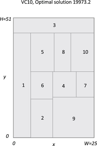
Figure 2. BA12, Optimal solution 8021.0.

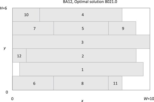
Figure 3. BA14, Best found solution 4628.5.

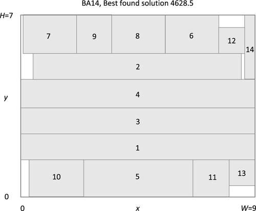
Figure 4. BA14B, Best found solution 4714.3.

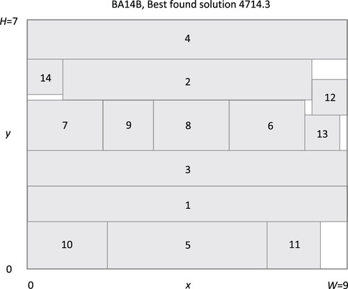
Table 5. Verified optimal solution, 19973.2, of VC10 solved in FLP3 form using PECP.

i	$x_i$	$y_i$	$w_i$	$h_i$
1	2.668161	22.3	5.336323	44.6
2	8.749750	8.202884	6.826854	16.405768
3	12.5	47.8	25.0	6.4
4	15.830841	22.669147	7.335328	10.906119
5	8.978023	36.362090	7.283401	16.475820
6	8.749750	22.264974	6.826854	11.718411
7	22.249252	22.669147	5.501495	10.906119
8	15.198948	36.361103	5.158449	16.477794
9	18.581588	8.608044	12.836823	17.216088
10	21.389086	36.361103	7.221828	16.477794

Table 6. Verified optimal solution, 8021.0, of BA12 solved in FLP3 form using PECP.

i	$x_i$	$y_i$	$w_i$	$h_i$
1	5.0	1.5	9.0	1.0
2	5.0	2.5	8.0	1.0
3	5.0	3.5	10.0	1.0
4	5.0	5.5	6.0	1.0
5	5.0	4.5	4.0	1.0
6	1.5	0.5	3.0	1.0
7	1.5	4.5	3.0	1.0
8	5.0	0.5	4.0	1.0
9	8.0	4.5	2.0	1.0
10	1.0	5.5	2.0	1.0
11	7.5	0.5	1.0	1.0
12	0.5	2.5	1.0	1.0

Table 7. Best found solution, 4628.5, of BA14 solved in FLP3 form using PECP.

i	$x_i$	$y_i$	$w_i$	$h_i$
1	4.5	1.928447	9.0	1.0
2	4.5	5.039558	8.0	1.0
3	4.5	2.928447	9.0	1.0
4	4.5	3.984003	9.0	1.111111
5	4.5	0.714224	4.2	1.428447
6	6.553401	6.269779	2.052898	1.460442
7	1.077375	6.269779	2.052744	1.460442
8	4.5	6.269779	2.053904	1.460442
9	2.788398	6.269779	1.369301	1.460442
10	1.35	0.714224	2.1	1.428447
11	7.3	0.714224	1.4	1.428447
12	8.079850	6.039558	1.0	1.0
13	8.5	0.928447	1.0	1.0
14	8.796954	5.769779	0.406091	2.460442

Table 8. Best found solution, 4714.3, of BA14B solved in FLP3 form using PECP.

i	$x_i$	$y_i$	$w_i$	$h_i$
1	4.5	1.833333	9.0	1.0
2	4.5	5.317535	7.0	1.142709
3	4.5	2.833333	9.0	1.0
4	4.5	6.444444	9.0	1.111111
5	4.5	0.666666	4.5	1.333333
6	6.723833	4.039757	2.123372	1.412847
7	1.061672	4.039757	2.123345	1.412847
8	4.600465	4.039757	2.123363	1.412847
9	2.831064	4.039757	1.415439	1.412847
10	1.125	0.666667	2.25	1.333333
11	7.499457	0.666667	1.498914	1.333333
12	8.5	4.833333	1.0	1.0
13	8.285519	3.833333	1.0	1.0
14	0.5	5.388889	1.0	1.0

The VC10 problem was solved in the FLP3 form to a verified optimal solution (using ${ϵ}_g=0.0001$) in 154 iterations (msl = 38). The optimal solution was found at iteration 149 (msl = 34). The BA12 problem was solved in the FLP3 form to a verified optimal solution (using ${ϵ}_g=0.000001$) in 44 iterations (msl = 27). The optimal solution was found at iteration 29 (msl = 14). The best found solution of the BA14 problem solved in FLP3 form was found after 73 iterations (msl = 33). The best found solution of the BA14B problem solved in FLP3 form was found after 86 iterations (msl = 48). However, problems BA14 and BA14B could not be solved to a verified optimal solution because of limitation in memory space for the MILP subsolver.

In Table 9 the results, when solving VC10, BA12, BA14 and BA14B in FLP3 form, with the PECP algorithm are summarized. Equal or almost equal solution results to the considered FLPs have, though, been found by genetic [32] and tabu search [30] algorithms some years ago. In Table 9 we have summarized results from some papers where the considered FLPs have been solved together with our results when solving the problems with PECP, ECP and ESH in the smooth convex FLP3 form. From the table it is found that genetic and tabu search algorithms are very efficient in finding good feasible solutions for FLPs. However, genetic and tabu search algorithms lack the property of verifying if an obtained solution, is optimal or not, while the PECP algorithm has this property. From the results in Table 9 it is, though, found that the final verification of optimality was very time consuming even if the problems were solved in smooth convex FLP3 form. However, the solution points given in Tables 5 and 6, obtained with PECP, are the global optimal ones and to the authors knowledge this is the first time ever, that proven global optimal solutions to these problems have been published. The problems BA14 and BA14B could, however, not be solved to global optimality with the PECP algorithm in the FLP3 form. These solution results are, given in Tables 7 and 8 as well as illustrated in the Figures 3 and 4. These solutions with PECP are the best solutions published as far as the authors know. All the results with PECP in Tables 5–9 were obtained by solving the problems in smooth convex FLP3 form in order to obtain a comparison with the results in [29], where this formulation initially was used. The ECP method used in this paper correspond to the ECP solution method in [29] but it has, though, been solved with a faster computer and a newer version of the MILP subsolver CPLEX in the ECP algorithm.

Table 9. Results when solving four challenging facility layout design problems.

Reference	Method	VC10	BA12	BA14	BA14B	Comments
Castillo et al. [29]	FLP3-ECP-MINLP	21298.0	8080.0	4919.5*		Objective
		26637	1667	6493*		CPU time found sol. (s)
Liu and Meller [39]	GA with MIP	19997.0	8702.0	5004.0		Objective
		–	–	–	–	CPU time found sol. (s)
Scholz et al. [30]	STaTS	19994.1	8264.0	4712.3		Objective
		9	14	16		CPU time found sol. (s)
Kulturel-Konak and Konak [31]	ACO-FBS	21463.1	8083.0	4739.7	4739.7	Objective
		34	67	531	262	CPU time found sol. (s)
Zarali et al. [35]	ACO		7715.0	4165.2		Objective
			–	–		CPU time found sol. (s)
Goncalves and Resende [32]	BRKGA-LP	19951.2	8021.0	4628.8		Objective
		46	114	160		CPU time found sol. (s)
		0.0016	0	0.0095		%$E_{max}$
This paper (2020)	FLP3-PECP-MINLP	19973.2	8021.0	4628.5	4714.3	Objective
		19166	627	5101	3701	CPU time found sol. (s)
		22435	13257	–	–	CPU time optimal (s)
		0.00019	0	0.084	0.073	%$E_{max}$
This paper (2020)	FLP3-ECP-MINLP	19972.6	8075.0	4721.9	4828.1	Objective
		28586	6109	7908	9855	CPU time found sol. (s)
		30777	–	–	–	CPU time optimal (s)
		0.00060	0	0.082	0.073	%$E_{max}$
This paper (2020)	FLP3-ESH-MINLP	19972.9	NA	NA	NA	Objective
		53382				CPU time found sol. (s)
		54943				CPU time optimal (s)
		0.00053				%$E_{max}$

Notes: The row ‘CPU time found sol.’ corresponds to the time needed to find the final solution. The ‘CPU time optimal’ corresponds to the time needed to find and verify optimality of the final solution. The accuracy measure %$E_{max}$ is defined in (2(2) $E_{max}=\underset{i=1,\dots ,N}{max}\frac{|A_i-w_i{h}_i|}{A_i}\cdot 100\mathrm{\%}.$(2) ). In [29] problem BA13 was solved instead of BA14. The results marked with * are, thus, not fully comparable. However, BA13 is a version of BA14 without considering department 14, which does not have any shape restriction and interaction with the other departments in BA14 [31,38].

In the final rows of Table 9 the results using the ECP and ESH methods are included as well. From the table it is found that the VC10 problem could also be solved to a verified optimal solution with the ECP and ESH methods, but the required CPU time was shorter for the PECP method. The feasibility problem in ESH could be solved with the algorithm in [12] in a fraction of a second, resulting in a RHS of the constraints equal to $-16.8$. But the total CPU time to solve the VC10 problem was magnitudes longer and also much longer than with PECP. Surprisingly, no other of the considered FLP-problems could be solved with ESH. The reason for this is that no relaxed interior points ${\mathit{x}}_f\in \{\mathit{x}\in X\mid \mathit{g}(\mathit{x})<\mathbf{0}\}$ can be found for the problems BA12, BA14 and BA14B. One could use the technique of [23] to create approximate interior points but this is sensitive to numerical accuracies which might be hard to deal with. Supporting hyperplanes can, therefore, not be generated at points ${\mathit{x}}_s\in \{\mathit{x}\mid \tilde{g}(\mathit{x})=0\wedge \mathit{x}\in [{\mathit{x}}_f,{\mathit{x}}_k\left]\right\}$ by using a line-search procedure. All relaxed feasible, as well as all integer feasible solutions for the problems BA12, BA14 and BA14B are, thus, found on the boundary of $L\cap C$. One reason for the lack of an interior point on those problems is that for i = 12 the width and height of the department is constrained to 1. Thus the nonlinear constraints (C1) and (C2) are always active for i = 12. From Table 9 it is, furthermore, found that the BA12 problem could not be solved to the same solution with ECP as with PECP and ECP could not verify an optimal solution, because of limitation in memory space for the B&B tree in the MILP subsolver. This was also the case when solving the BA14 and BA14B problems with both ECP and PECP. The solutions found with PECP where, though, better with PECP than with ECP.

As ECP, PECP and ESH are able to solve smooth and nonsmooth convex MINLP problems to optimality we did also a small comparative study with the problem VC10 to find out in which form (FLP2) or (FLP3) and by which approach (ECP, PECP or ESH) this FLP is most efficiently solved. In the comparison we used the parameter values: ${\mathrm{m}\mathrm{s}\mathrm{l}}_0=1$ and ${ϵ}_g=0.001$ in ECP, PECP and ESH as well as ${ϵ}_P=1$ and P = 3 in PECP. The results are given in Table 10, where one finds that the problem VC10 was solved to global optimality with ECP, PECP and ESH using both the nonsmooth convex FLP2 and the smooth convex FLP3 form of the problem. From Table 10 it is found that the VC10 problem could be solved faster with PECP than with ECP or ESH and the problem was solved faster in the nonsmooth convex FLP2 form than in the smooth convex FLP3 form with all the methods. Since the smooth convex FLP3 formulation include linear expressions (LS1)–(LS4) for all $1\le i<j\le N$ while the nonsmooth convex FLP2 form include corresponding nonlinear inequalities (C3-NS) only for those $i,j\in \{i,j\mid c_{i,j}\ne 0\}$ one could assume that the formulation FLP3 would be faster if the linear expressions (LS1)–(LS4) would also be restricted to only those $i,j\in \{i,j\mid c_{i,j}\ne 0\}$. We call this more compact FLP3 formulation as FLP3c in Table 10. From the Table 10 we can see that the higher computational time of the FLP3 formulation compared to the FLP2 formulation can not be explained by a higher number of (LS1)–(LS4) constraints in the original FLP3 form than the corresponding number of (C3-NS) constraints in the FLP2 form where the tighter index set $i,j\in \{i,j\mid c_{i,j}\ne 0\}$ was used. From Table 10 it is also found that the MINLP problem VC10 was solved to global optimality by only solving one MILP subproblem to optimality in each of the cases with ECP and PECP.

Table 10. Results when solving VC10 in FLP2, FLP3 and FLP3c form by ECP, PECP and ESH (using ${ϵ}_g=0.001$).

Formulation	Algorithm	Objective	Iterations	msl	MILPs*	CPU time (s)	$g_{i,\mathrm{m}\mathrm{a}\mathrm{x}}$
Smooth convex FLP3	ECP	19966.5	162(161)	28(28)	1	13399(8933)	$g_4=0.00055$
Smooth convex FLP3c	ECP	19968.1	164(162)	30(28)	1	21219(16972)	$g_4=0.00054$
Smooth convex FLP3	PECP	19964.1	138(136)	22(21)	1	10167(8155)	$g_6=0.00092$
Smooth convex FLP3c	PECP	19969.7	148(147)	26(25)	1	14971(12797)	$g_6=0.00041$
Smooth convex FLP3	ESH	19965.9	434(434)	18(18)	3	31789(31789)	$g_2=0.00089$
Nonsmooth convex FLP2	ECP	19968.4	129(129)	15(15)	1	9768(9768)	$g_9=0.00052$
Nonsmooth convex FLP2	PECP	19972.9	126(125)	18(18)	1	6422(4249)	$g_6=0.000064$
Nonsmooth convex FLP2	ESH	19966.9	454(454)	18(18)	9	26942(26942)	$g_3=0.00064$

Notes: The values within the parentheses correspond to those when the optimal solution first was found while the values in front of the parentheses correspond to the values at termination when the solutions were verified to be optimal.

From Table 10 it is found that the number of iterations is higher with ESH than with ECP and PECP. This has its explanation in that the number of supports generated per iteration with ESH is much lower than the number of cuts that can be generated per iteration with ECP and PECP. When using ESH, it was found that a maximum of two supports could be generated and added in a few iterations while only one could be added in the other iterations. The final polytope $L_k$ approximating the relaxed feasible region, $L\cap C$, (in the problem $\left(P_k\right)$) was, thus, obtained with a higher k-value and a higher total computational load with ESH than with ECP and PECP. Furthermore, it is notable that the CPU time needed to build up the final polytope, $L_k$, and the final MILP problem, $P_k$, was in some cases shorter than the CPU time needed to solve the final MILP problem, $P_k$, once to optimality This has an additional value, because not only an optimal solution result is obtained for each case, but also a final MILP problem, $P_k$, wherefrom the solution can be obtained.

In connection to all results it should be mentioned that when comparing our solution results with those given in other papers we found that even better solution results than our optimal solutions have been reported. However, in the papers, where better solutions than ours were found, we also found differencies in the parameters or in the formulation used, explaining this discrepancy. For example, Zarali et al. [35] reported a solution (with the objective function value) 7715.03 on the instance BA12, while the (global optimal) solution we obtained, has an objective function value equal to 8021.0 with at least 6 decimals accuracy. But, when considering the solution in [35], we found that the authors have used a total facility area of $7\cdot 9=63$, while the total facility area for the BA12 problem in [36] was $6\cdot 10=60$. In addition Zarali et al. [35] used euclidean distances between the departments in the objective function and not rectilinear. Using a rectilinear distances criteria the solution of BA12 in [35] would have been 9703. The best solution value 4165.24 on the objective function for the instance BA14 found in [35] was, as well, much lower than the best found solution value 4628.5 we obtained. However, also in this case, Zarali et al. [35] has used euclidean distances in the objective function. Thus, these solution values are not comparable.

We found, furthermore, some smaller, but clearly notable, differences between our solution results and earlier reported ones. We found, though, that some of these differences could be explained by different solution accuracy only. For example, Goncalves and Resende [32] reported a best known solution 19951.2 to the problem VC10 from [37] while we report a global optimal solution with the objective function value equal to 19973.2. When solving this problem with different accuracies, we found that it is, most probably, the accuracy that has been used by Goncalves and Resende [32] that makes the difference. When we solved the VC10 problem to optimality with different accuracy, we obtained optimal objective function values of the problem between 19933.5 and 19973.2. These solution results are given in Table 11. It may be noted that the results in Table 11 correspond to those when solving the VC10 problem in the smooth convex FLP3 form. The computational times are slightly lower in case the nonsmooth FLP2 form is used. The accuracy measured as the maximum relative error (in percentage) of any department area is a simple measure, given in the papers [29,32]. This accuracy measure is calculated as follows, (2) $E_{max}=\underset{i=1,\dots ,N}{max}\frac{|A_i-w_i{h}_i|}{A_i}\cdot 100\mathrm{\%}.$(2) For the solutions between 19933.5 to 19973.2 the $E_{max}$ value was between 0.2 % and 0.0002 % in our calculations, as can be found in Table 11. According to these results, a solution with an objective function value equal to 19951.7, would, most likely have an $E_{max}$ value close to 0.05%. Thus we feel the solution reported in [31], would, in principle, be the same as ours, but obtained with a lower accuracy.

Table 11. Optimal results when solving VC10 in FLP3 form with PECP using different ${ϵ}_g$.

${ϵ}_g$	Objective	Iterations	CPU time (s)	msl	$g_{i,\mathrm{m}\mathrm{a}\mathrm{x}}$	$E_{max}\left(\mathrm{\%}\right)$
0.1	19933.5	44	4977	22	$g_1=0.052$	0.17
0.01	19954.8	82	6748	25	$g_6=0.0057$	0.052
0.001	19964.1	138	10167	22	$g_6=0.00092$	0.0079
0.0001	19973.2	154	22435	38	$g_2=0.000032$	0.00019

Note: $E_{max}\left(\mathrm{\%}\right)$ is the accuracy measure defined in (2(2) $E_{max}=\underset{i=1,\dots ,N}{max}\frac{|A_i-w_i{h}_i|}{A_i}\cdot 100\mathrm{\%}.$(2) ).

As the parameters, for the considered instances may deviate in different papers we report in the appendix the values of all parameters and restrictions that we have used for the instances VC10, BA12, BA14 and BA14B. From the appendix it can also be observed that the only difference between the instances BA14 and BA14B is the restrictions on the width and length of the 14th department which are restricted to $w_{min}=l_{min}=1$ in the problem BA14B while they are not resticted at all in the problem BA14. We report, for comparison, our results for both these cases, because this problem has been solved with and without restrictions on the width and length of the department 14 in several papers, without mentioning which formulation has been used.

6. Conclusions

In this paper it was shown that projected cutting planes can be an attractive alternative in optimization algorithms using cutting planes and especially in the extended cutting plane algorithm. The algorithm was proven to converge to a global optimum for both smooth and nonsmooth convex MINLP problems. The computational efficiency of the algorithm was, further, demonstrated by solving some very difficult facility layout problems to global optimality. To the authors knowledge this is the first time when it has been shown that the considered facility layout problems, VC10 and BA12, have been solved to global optimality.

Disclosure statement

No potential conflict of interest was reported by the author(s).

Correction Statement

This article has been republished with minor changes. These changes do not impact the academic content of the article.

Appendix. Initial data to facility layout problems

Table A1. Initial data.

Problem	N	W	H	Facility requirements	Source
VC10	10	25	51	$w_{min}=h_{min}=5$	van Camp et al. [37]
BA12	12	10	6	$w_{min}=h_{min}=1$	Bazaraa [36]
BA14	14	9	7	$w_{min}=h_{min}=1^{\ast }$	Bazaraa [36]
BA14B	14	9	7	$w_{min}=h_{min}=1$	Bazaraa [36]

*For all departments except for the last facility in BA14 which is not restricted.

Table A2. Initial data.

Problem	N	$(A_i,i=1,\dots ,N)$
VC10	10	(238,112,160,80,120,80,60,85,221,119)
BA12	12	(9,8,10,6,4,3,3,4,2,2,1,1)
BA14	14	(9,8,9,10,6,3,3,3,2,3,2,1,1,1)
BA14B	14	(9,8,9,10,6,3,3,3,2,3,2,1,1,1)

Table A3. Initial data.

-VC10-
$(i,j)$	$c_{i,j}$
(1,6)	218	(2,6)	148	(2,9)	296	(3,4)	28	(3,5)	70	(4,6)	28	(4,7)	70
(4,8)	140	(5,8)	210	(7,10)	28	(8,10)	888	(9,10)	59.2
-BA12-
$(i,j)$	$c_{i,j}$
(1,2)	288	(1,3)	180	(1,4)	54	(1,5)	72	(1,6)	180	(1,7)	27	(1,8)	72
(1,9)	36	(1,12)	9	(2,3)	240	(2,4)	54	(2,5)	72	(2,6)	24	(2,7)	48
(2,8)	160	(2,9)	16	(2,10)	64	(2,11)	8	(2,12)	16	(3,4)	120	(3,5)	80
(3,7)	60	(3,8)	120	(3,9)	60	(3,12)	30	(4,5)	72	(4,6)	18	(4,7)	18
(4,8)	48	(4,9)	24	(4,10)	48	(4,11)	12	(5,6)	12	(5,7)	12	(5,8)	64
(5,9)	16	(5,10)	16	(5,11)	4	(5,12)	8	(6,7)	18	(6,8)	24	(6,9)	6
(6,10)	12	(6,11)	3	(6,12)	3	(7,9)	6	(7,10)	6	(7,11)	3	(7,12)	6
(8,9)	16	(8,10)	16	(8,11)	16	(8,12)	4	(9,10)	4	(9,11)	4	(9,12)	2
(10,11)	2	(10,12)	2	(11,12)	2
-BA14-	and	-BA14B-
$(i,j)$	$c_{i,j}$
(1,2)	72	(1,3)	162	(1,4)	90	(1,5)	108	(1,6)	27	(1,9)	18	(1,10)	27
(1,11)	18	(2,3)	72	(2,4)	80	(2,6)	48	(2,8)	48	(2,9)	32	(2,11)	16
(2,12)	8	(3,4)	45	(3,5)	54	(3,6)	27	(3,7)	27	(3,8)	27	(3,10)	27
(3,12)	9	(3,13)	18	(4,5)	30	(4,7)	30	(4,8)	30	(4,9)	20	(4,11)	20
(4,12)	10	(4,13)	10	(5,6)	18	(5,8)	18	(5,9)	12	(5,10)	18	(5,11)	24
(6,7)	9	(6,8)	9	(6,11)	6	(6,12)	6	(6,13)	6	(7,8)	9	(7,9)	12
(7,10)	9	(7,11)	6	(7,12)	3	(8,9)	6	(8,10)	9	(8,12)	3	(9,10)	6
(9,11)	4	(9,12)	6	(9,13)	2	(10,11)	6	(10,12)	3	(10,13)	6	(11,12)	2
(12,13)	4

References

- Duran M, Grossmann IE. An outer approximation algorithm for a class of mixed-integer nonlinear programs. Math Program. 1986;36:307–339.
- MINLP Library 2. Mixed-integer nonlinear programming library; 2020. Available from: http://www.minlplib.org/
- Bussieck MR, Vigerske S. MINLP solver software. In Wiley encyclopedia of operations research and management science;. 2010. doi:10.1002/9780470400531.eorms0527.
- Bonami P, Kilinic M, Linderoth J. Algorithms and software for convex mixed integer nonlinear programs. In: Lee J, Leyffer S, editors. Mixed integer nonlinear programming. The IMA volumes in mathematics and its applications, Vol. 154. New York: Springer; 2012. p. 1–39.
- Westerlund T, Pettersson F. An extended cutting plane method for solving convex MINLP problems. Comput Chem Engin Sup. 1995;19:131–136.
- Kelley JE. The cutting plane method for solving convex programs. J SIAM. 1960;8:703–712.
- Westerlund T, Skrifvars H, Harjunkoski I, et al. An extended cutting plane method for a class of non-convex MINLP problems. Comput Chem Eng. 1998;22:357–365.
- Westerlund T, Pörn R. Solving pseudo-convex mixed integer optimization problems by cutting plane techniques. Optim Eng. 2002;3:253–280.
- Eronen VP, Mäkelä MM, Westerlund T. On the generalization of ECP and OA methods to nonsmooth convex MINLP problems. Optimization. 2014;63:1057–1073.
- Eronen VP, Mäkelä MM, Westerlund T. Extended cutting plane method for a class of nonsmooth nonconvex MINLP problems. Optimization. 2015;64:641–661.
- Eronen VP, Kronqvist J, Westerlund T, et al. Method for solving generalized convex nonsmooth mixed-integer nonlinear programming problems. J Global Optim. 2017;69:443–459.
- Westerlund T, Eronen V-P, Mäkelä MM. On solving generalized convex MINLP problems using supporting hyperplane techniques. J Global Optim. 2018;71:987–1011.
- Horst R, Tuy H. Global optimization. 3rd ed. Heidelberg: Springer-Verlag; 1996.
- Pörn R. Mixed integer non-linear programming: convexification techniques and algorithm development [PhD thesis]. Abo Akademi University; 2000.
- Censor Y, Lent A. Cyclic subgradient projections. Math Program. 1982;24:233–235.
- Bauschke HH, Borwein JM. On projection algorithms for solving convex feasibilty problems. SIAM Rev. 1996;38:367–426.
- Bauschke HH, Combettes PL. A weak-to-strong convergence principle for Fejér-monotone methods in Hilbert spaces. Math Oper Res. 2001;26:248–264.
- D'Antonio GH, Frangioni F. Convergence analysis of deflated conditional approximate subgradient methods. SIAM J Optim. 2009;20:357–386.
- IBM ILOG Optimization Studio. CPLEX User's Manual, version 12.7. IBM; 2017.
- Gurobi. Gurobi optimizer reference manual. version 9.0. Gurobi Optimization, LCC; 2020.
- Emet S, Westerlund T. Comparisons of solving a chromatographic separation problem using MINLP methods. Comput Chem Eng. 2004;28:673–682.
- Serrano F, Schwarz R, Gleixner A. On the relation between the extended supporting hyperplane algorithm and Kelley's cutting plane algorithm. J Global Optim. 2020;78:161–179.
- Kronqvist J, Lundell A, Westerlund T. The extended supporting hyperplane algorithm for convex mixed-integer nonlinear programming. J Global Optim. 2016;64:249–272.
- Veinott Jr AF. The supporting hyperplane method for unimodal programming. Oper Res. 1967;15:147–152.
- Westerlund T. User's guide for GAECP, version 5.537. An interactive solver for generalized convex MINLP-problems using cutting plane and supporting hyperplane teqniques. Abo Akademi University. 2017. Available from: http://www.abo.fi/twesterl/GAECPDocumentation.pdf
- Mäkelä MM, Neittaanmäki P. Nonsmooth optimization: analysis and algorithms with applications to optimal control. Singapore: World Scientific Publishing Co.; 1992.
- Bagirov A, Karmitsa N, Mäkelä MM. Introduction to nonsmooth optimization. Heidelberg: Springer Cham; 2014. (Theory, practice and software).
- Fletcher R, Leyffer S. Solving mixed integer nonlinear programs by outer approximation. Math Program. 1994;66:327–349.
- Castillo I, Westerlund J, Emet S, et al. Optimization of block layout design problems with unequal areas: a comparison of MILP and MINLP optimization methods. Comput Chem Engin. 2005;30:54–69.
- Scholz D, Petrick A, Domschke W. STaTS: A slicing tree and tabu search based heuristic for unequal area facility layout. Eur J Oper Res. 2009;197:166–178.
- Kulturel-Konak S, Konak A. Unequal area flexible bay facility layout using ant colony optimization. Int J Product Optim. 2011;49:1877–1902.
- Goncalves JF, Resende MGC. A biased random-key genetic algorithm for unequal area facility layout problem. Eur J Oper Res. 2015;246:86–107.
- Konak A, Kulturel-Konak S, Norman BA, et al. A new mixed integer programming formulation for facility design using flexible bays. Oper Res Lett. 2006;34:660–672.
- Kronqvist J, Lundell A, Westerlund T. Reformulations for utilizing separability when solving convex MINLP problems. J Global Optim. 2018;71:571–592.
- Zarali F, Yazagan HR, Delice Y. A new solution method of ant colony-based logistic center area layout problem. Sãdhanã. 2018;83:1–17.
- Bazaraa MS. Computerized layout design; a branch and bound approach. AIIE Trans. 1975;7:432–438.
- van Camp DJ, Carter MW, Vanelli A. A nonlinear optimization approach for solving facility layout problems. Eur J Oper Res. 1991;57:174–189.
- Castillo I, Westerlund T. An epsilon-accurate model for optimal unequal-area block layout design. Comput Oper Res. 2005;32:429–447.
- Liu Q, Meller RD. A sequence-pair representation and MIP-model-based heuristic for the facility layout problem with rectangular departments. IIE Trans. 2007;39:377–394.