An adaptive patch approximation algorithm for bicriteria convex mixed-integer problems

Abstract

Pareto frontiers of bicriteria continuous convex problems can be efficiently computed and optimal theoretical performance bounds have been established. In the case of bicriteria mixed-integer problems, the approximation of the Pareto frontier becomes, however, significantly harder. In this paper, we propose a new algorithm for approximating the Pareto frontier of bicriteria mixed-integer programs with convex constraints. Such Pareto frontiers are composed of patches of solutions with shared assignments for the discrete variables. By adaptively creating such a patchwork, our algorithm is able to create approximations that converge quickly to the true Pareto frontier. As a quality measure, we use the difference in hypervolume between the approximation and the true Pareto frontier. At least a certain number of patches is required to obtain an approximation with a given quality. This patch complexity gives a lower bound on the number of required computations. We show that our algorithm performs a number of optimization steps that are of a similar order as this lower bound. We provide an efficient MIP-based implementation of this algorithm. The efficiency of our algorithm is illustrated with numerical results showing that our algorithm has a strong theoretical performance guarantee while being competitive with other state-of-the-art approaches in practice.

Keywords:

• Bicriteria optimization
• mixed-integer programming
• approximation
• rate of convergence

AMS Classifications:

• 90C29
• 90C11
• 90C59
• 90-08

1. Motivation and concepts

Optimization problems, in practice, naturally have multiple conflicting goals. To identify optimal trade-offs with respect to these goals, multicriteria optimization aims to compute the corresponding Pareto frontiers. For these applications, the ability to compute efficiently a good approximation to the Pareto frontier is needed. Some methods for this approximation are surveyed in [1]. A large fraction of models for typical real-world decision problems are mixed-integer programs that integrate discrete with continuous decision variables. In industrial applications, the number of continuous variables typically clearly dominates the number of discrete variables. Existing algorithms for bicriteria optimization of mixed-integer programs are able to compute approximations of the Pareto frontier ([2–4]). Although for many of these algorithms it is known that their results converge to the true Pareto frontier, state-of-the-art methods do not provide specific bounds on the convergence speed. Asymptotically optimal bounds for the number of optimization steps needed to compute the exact Pareto frontier are only known for algorithms on pure integer problems in the case of two [5] and three criteria [6].

For the simpler case without discrete variables, however, approximation algorithms for continuous convex bicriteria problems with strong guarantees on the convergence speed have been established [7]. This bound of $O\left(1/n^2\right)$ on the Hausdorff distance after n optimization steps is asymptotically optimal since any approximation with n segments of a convex two-dimensional set has an error of $\mathrm{\Omega }\left(1/n^2\right)$ in the worst-case [8]. In this paper, we give an analogous result for convex mixed-integer programs, which is, however, instance-specific. We present an algorithm that only needs a number of optimization steps of the same order as the number of parts necessary to represent an approximation of the obtained quality.

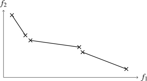
We consider bicriteria mixed-integer programs with constraints that are convex in the continuous variables, i.e. each constraint can be represented by an inequality $g(c,d)\le 0$ where the function g is convex in the continuous variables $c\in {\mathbb{R}}^k$ for each fixed choice of the discrete variables $d\in {\mathbb{Z}}^m$. Thus, we can create convex combinations of feasible points with shared values d for the discrete variables while still maintaining feasibility. This shows that we can create a segment of attainable vectors in objective space by taking the corresponding objective vectors as endpoints. We will refer to this as a segment patch in the following. In Figure 1, some segment patches are shown.

Figure 1. An illustration of three patches in objective space.

As an approximation quality measure, we use a measure based on the hypervolume [9]. This difference volume measure is given by the volume of the region between the true Pareto frontier and the approximation. The use of this measures enable an adaptive choice on the number of patches used in different regions of the Pareto frontier. In areas where a single patch is already close to the true Pareto frontier, no further patches are needed. This distinguishes our approach from classical considerations of the approximation quality where uniform grids on the nondominated set are required which leads to restrictions on the efficiency [10].

Our algorithm iteratively computes patches that are then added to the approximation. The computation of the new patch is done adaptively based on the current approximation to ensure a maximal improvement of the difference volume.

Our convergence analysis is done on a per-instance basis which allows for more fine-grained results than a global worst-case analysis. We show that the number of optimization steps required by our algorithm for a bicriteria programming instance is of a similar order as the number of patches required to represent an approximation to the corresponding Pareto frontier with the given quality. This theoretical analysis is combined with numerical evaluations on benchmarks that show that the practical efficiency of our algorithm is competitive with other state-of-the-art algorithms.

1.1. Related work

A large number of multicriteria optimization methods have been developed. However, the still large amount of new methods proposed in the recent years shows that current algorithmic techniques are not yet satisfactory in all application areas. We describe here a non-exhaustive subset of the methods in the literature to illustrate the main research directions.

Our considered problems of bicriteria convex mixed-integer problems form a subset of the general nonlinear bicriteria case, for which several methods are known [11–13]. These algorithms are, however, unable to use the specific structure created by mixed-integer problems. A special case of convex MIPs are linear MIPs for which there is a larger set of methods available in the literature. Available algorithms for computing Pareto frontiers of bicriteria mixed-integer programs (Bicriteria MIPs) can be classified into two types:

• Algorithms based on branch-and-bound that perform recursive branching on some variables. Such an algorithm for the convex case is considered in [14], while [15–17] propose algorithms for the linear case.

• Algorithms based on scalarization which generates special scalarized MIPs that are then solved to optimality to obtain a new point and corresponding information about the Pareto frontier. The papers [2,18] discuss the convex case, while [3,4,19] focus on the linear case.

Only a small number of algorithms aim to compute approximations for which explicit quality guarantees were shown. For example, the work [20] provides an algorithm which is guaranteed to output ε-approximate Pareto frontiers. For most algorithms, the approximation quality can only be controlled indirectly and no analysis of the provided guarantees in terms of widely-used quality measures is available.

Previous approaches using patches

A limited number of works in multicriteria optimization use the concept of a patch.

The notion of patches in multicriteria optimization is introduced in [21] along with applications to radiotherapy planning. Patches were used for performing a Pareto-navigation over the set of solutions of a multicriteria radiotherapy planning problem in [22].

In [17], the concept of a slice is presented which is similar to our concept of a patch. A bicriteria optimization problem is reduced to slice problems. For a fixed assignment to the discrete variables, a corresponding feasible assignment to the continuous variables is computed. The assignment to the discrete variables is, however, fixed before, and not chosen adaptively as in our approach.

Patches are used implicitly in [15,23]. In this approach, after fixing the discrete variables, extreme Pareto points of the obtained continuous multicriteria problem are computed. The convex hull of these extreme points, which corresponds to a patch, is used for checking Pareto-efficiency. A correction to this check of Pareto-efficiency is provided in [24] along with some further improvements of the algorithm. In [19] a patch is implicitly computed in a line detection step, however only with fixed objective values.

1.2. Motivation and goals for our algorithm

Deficits of current approaches

All of the discussed algorithms for bicriteria mixed-integer programs have the following properties in common:

• The algorithms do not provide clear guarantees of the approximation quality provided by the output in terms of widely used quality measures.

• There is no comprehensive theoretical analysis of the running time of the algorithms as a function of the approximation quality. The implicit limits on the approximation quality imposed by the choice of parameters or early stopping are not analysed.

The characteristics of our approach

In this paper, we develop an algorithm which is designed contrarily to the above characteristics. We pose the following goals to achieve with our method:

• The approximation returned by the algorithm in each step should be an inner approximation, i.e. all points in the approximation should correspond to feasible solutions that can be directly computed.

• The algorithm should provide an approximation of the Pareto frontier with a clearly quantified approximation guarantee at every step. In particular, the algorithm can be stopped at every moment and we still obtain a result with a clear approximation guarantee, i.e. the algorithm should be an anytime algorithm [25]. The approximation quality obtained until each given time limit should be competitive with every other algorithm that requires a similar amount of time.

• The approximation quality obtained by the algorithm, respectively, the needed number of iterations to reach some given accuracy, should be bounded with respect to some intrinsic property of the problem we solve. In particular, the performance of the algorithm should be not too far away from a theoretical optimum that is given by the number of patches minimally needed to describe an approximation to the Pareto frontier.

1.3. Results and organization of this paper

In Section 2, we describe the basic concepts of multicriteria optimization and approximation of Pareto frontiers. We describe the concept of a patch and introduce the difference volume as our approximation quality measure. This leads to the notion of patch complexity that measures the complexity for approximating the Pareto frontier inherent to a problem. We then introduce in Section 3 the adaptive patch approximation algorithm and establish a corresponding convergence result based on the patch complexity. The proven upper bound on the number of iterations is of the same order as the lower bound given by the patch complexity. In the subsequent Section 4, we describe how the iterations of the adaptive patch approximation algorithm can be realized. We provide a mixed-integer programming formulation for finding an optimal patch with only about twice the number of variables and constraints of the original mixed-integer program. We show that it is sufficient to solve a constant number of these mixed-integer programs per iteration.

The developed algorithm is evaluated numerically in Section 5 using several benchmark problems from the literature. The results show that the running time of our algorithm is competitive with other state-of-the-art approaches.

2. The complexity of approximating pareto frontiers with patches

2.1. Bicriteria convex mixed-integer problems

Our algorithm works with arbitrary bicriteria convex mixed-integer problems. In the following we characterize this problem class and discuss the corresponding theoretical notions. For a comprehensive theoretical introduction to the topic of multicriteria optimization, see [26].

We present here the general case of $K\in \mathbb{N}$, $K\ge 2$ criteria although our algorithm will focus later on the case K = 2. A general multicriteria program has the form $\begin{array}{r}\min f\left(x\right)\\ \mathrm{s}.\mathrm{t}.x\in X\end{array}$ where X is an arbitrary nonempty set and f is a vector-valued function $f:X\to {\mathbb{R}}^K$ with components $f\left(x\right)=\left(f_1\right(x),\dots ,f_K(x){)}^T$. We assume throughout this paper that all objectives should be minimized. Our algorithm treats the case of bicriteria mixed-integer convex programs, i.e. there are K = 2 criteria and the feasible set X in decision space can be represented in the form (1) $X=\left\{(c,d)\in {\mathbb{R}}^k\times {\mathbb{Z}}^m\mid g_i(c,d)\le 0\mathrm{f}\mathrm{o}\mathrm{r}\mathrm{e}\mathrm{a}\mathrm{c}\mathrm{h}i\in I\right\}$(1) where the functions $g_i$, $i\in I$ are convex w.r.t. $c\in {\mathbb{R}}^k$ for each fixed $d\in {\mathbb{Z}}^m$. We consider here the case that each of the component objective functions $f_i$, $i=1,\dots ,n$ is an affine linear function. Note that when solving minimization tasks, this restriction to linear objective functions instead of general convex objective functions does not reduce the class of problems that we can model. A convex objective function can be replaced by a new variable and the objective function shifted into the constraints. This class of problems also contains the widely considered class of bicriteria mixed-integer linear programs.

We use the ordering cone ${\mathbb{R}}_{\ge 0}^K$ to describe a dominance relation between two multicriteria objective vectors $z^{\left(1\right)}\in {\mathbb{R}}^K$ and $z^{\left(2\right)}\in {\mathbb{R}}^K$. The solution $z^{\left(1\right)}$ is said to dominate $z^{\left(2\right)}$ with respect to the ordering cone ${\mathbb{R}}_{\ge 0}^K$ if $z^{\left(2\right)}\in z^{\left(1\right)}+({\mathbb{R}}_{\ge 0}^K\setminus \{0\left\}\right)$.

Let $Z:=f\left(X\right)\subseteq {\mathbb{R}}^K$ be the (nonempty) set of all attainable vectors in objective space. The goal of multicriteria optimization is to compute (representations of) the set of nondominated objective vectors $N\left(Z\right)$. With respect to the ordering cone ${\mathbb{R}}_{\ge 0}^K$ this set is defined as $N\left(Z\right):=Z\setminus (Z+({\mathbb{R}}_{\ge 0}^K\setminus \left\{0\right\}\left)\right).$ The ordering cone ${\mathbb{R}}_{\ge 0}^K$ is used to describe the goal of minimization with respect to all objective functions $f_1\left(x\right),\dots ,f_K\left(x\right)$.

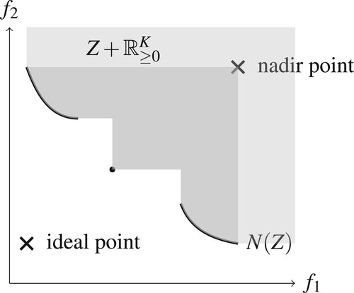
The nadir point of Z is given by the vector $z^N\left(Z\right)$ with components $z_i^N\left(Z\right):=sup\{z_i\mid z\in N(Z\left)\right\},i=1,\dots ,n$ representing the maximal trade-off that we can make in each component. The ideal point of Z is given by the vector $z^I\left(Z\right)$ with components $z_i^I\left(Z\right):=inf\{z_i\mid z\in Z\},i=1,\dots ,n$ representing the optimum that can be achieved in each objective function. Figure 2 illustrates a nondominated set with ideal and nadir point.

Figure 2. Illustration of the ideal point and nadir point in objective space. The thick curve and the dotted point represent the set of nondominated objective vectors.

2.2. Patches

The basis of our algorithm is formed by the concept of a patch. It makes use of the fact that the variables of a mixed-integer program can be decomposed into continuous and discrete parts.

Let $(c_1,d)\in X$ and $(c_2,d)\in X$ be two feasible points in decision space which share the values d for the discrete variables. Then, by the convexity of the constraint functions $g_i$ in the continuous variables it holds that every convex combination of the two points $(\lambda c_1+(1-\lambda )c_2,d)$ with $\lambda \in [0,1]$ fulfils $g_i(\lambda c_1+(1-\lambda )c_2,d)\le \lambda g_i(c_1,d)+(1-\lambda )g(c_2,d)\le 0$ and is thus also a feasible point contained in X. The corresponding objective vector can be written as $f(\lambda c_1+(1-\lambda )c_2,d)=\lambda f(c_1,d)+(1-\lambda )f(c_2,d)$ since we assume f to be affine linear. By varying $\lambda \in [0,1]$, we obtain a segment of attainable objective vectors, i.e. a segment patch with endpoints $f(c_1,d)$ and $f(c_2,d)$. By taking convex combinations of the two points $z^1\in f(c_1,d)+{\mathbb{R}}_{\ge 0}^K$ and $z^2\in f(c_2,d)+{\mathbb{R}}_{\ge 0}^K$ contained in the upper sets of these points, we can create an alternative segment. All vectors in this segment are also contained in the upper set $Z+{\mathbb{R}}_{\ge 0}^K$, since for each value $\lambda \in [0,1]$ the point on the alternative segment is dominated by the corresponding, attainable point on the original segment due to the component-wise inequality $\lambda z^1+(1-\lambda )z^2\ge \lambda f(c_1,d)+(1-\lambda )f(c_2,d).$ We formalize the concept of a patch in the following definition.

Definition 2.1

Segment patch in objective space

Let $(c_1,d)\in X$ and $(c_2,d)\in X$ be two (not necessarily distinct) feasible points in decision space with shared values for the discrete variables. Let $z^{\left(1\right)}\in f(c_1,d)+{\mathbb{R}}_{\ge 0}^K$ and $z^{\left(2\right)}\in f(c_2,d)+{\mathbb{R}}_{\ge 0}^K$ be two points that are contained in the upper sets of the corresponding objective vectors. Then, the line segment $\{\lambda z^{\left(1\right)}+(1-\lambda )z^{\left(2\right)}\mid \lambda \in [0,1\left]\right\}$ between $z^{\left(1\right)}$ and $z^{\left(2\right)}$ is a segment patch.

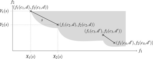
The simple representation of a segment patch by two vectors allows for an efficient search procedure by our algorithm. We use the symbol s to denote such a segment patch. In the case of two criteria, we denote the components of the two endpoints $z^{\left(1\right)}$ and $z^{\left(2\right)}$ by $X_1\left(s\right)=z_1^{\left(1\right)}$, $X_2\left(s\right)=z_1^{\left(2\right)}$ and $Y_1\left(s\right)=z_2^{\left(1\right)}$, $Y_2\left(s\right)=z_2^{\left(2\right)}$. An illustration of a set of segment patches in objective space is given in Figure 3.

Figure 3. Illustration of two segment patches in a two-dimensional objective space. The patch s corresponds to the discrete assignment d and has endpoints given as $\left(X_1\right(s),Y_1(s\left)\right)$ and $\left(X_2\right(s),Y_2(s\left)\right)$. Another patch corresponds to a different discrete assignment $d^{\prime }$. The grey background represents the upper set $Z+{\mathbb{R}}_{\ge 0}^2$ of attainable objective vectors.

Scaling Assumption

We require the following scaling assumption which is also used in [16]. This assumption is mainly used to simplify the analysis of the algorithm.

Assumption 2.1

Scaling

The nadir point and the ideal point have only finite components each. The objectives are scaled by an affine transformation such that the ideal point has coordinates $z^I=(0,\dots ,0{)}^T$ and the nadir point has coordinates $z^N=(1,\dots ,1{)}^T$.

2.3. Measures of approximation quality

In multicriteria optimization, a large number of measures of the approximation quality exist [27]. For obtaining convergence results, the choice of a measure with good theoretical properties is key.

2.3.1. Difference volume

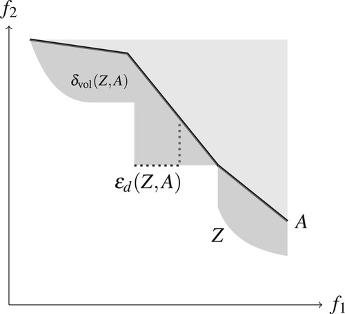
The difference volume aims to quantify the average error that the approximation has to the true Pareto frontier (Figure 4). We use this as the basis for both the construction and the analysis of our algorithm.

Definition 2.2

Difference volume

Let $A\subseteq Z$ be an approximation of the set of attainable objective vectors Z. Note that by our scaling assumption, it holds $Z\subseteq [0,1{]}^K$. The difference volume ${\delta }_{\mathrm{vol}}(Z,A)$ of Z and A with respect to the standard ordering cone ${\mathbb{R}}_{\ge 0}^K$ is defined as the enclosed volume between the upper sets $Z+{\mathbb{R}}_{\ge 0}^K$ and $A+{\mathbb{R}}_{\ge 0}^K$: $\begin{array}{rl}{\delta }_{\mathrm{vol}}(Z,A)& :=\mathrm{vol}\left(\left(\left(Z+{\mathbb{R}}_{\ge 0}^K\right)\setminus \left(A+{\mathbb{R}}_{\ge 0}^K\right)\right)\cap [0,1{]}^K\right)\\ & \stackrel{A\subseteq Z}{=}\mathrm{vol}\left(\left(Z+{\mathbb{R}}_{\ge 0}^K\right)\cap [0,1{]}^K\right)-\mathrm{vol}\left((A+{\mathbb{R}}_{\ge 0}^K)\cap [0,1{]}^K\right)\end{array}$

The difference volume is closely related to the hypervolume-measure [28] as it can be represented as the difference in hypervolume of the approximation and the true Pareto frontier. In [29] the related hyperarea difference is defined which is equivalent to the difference volume if a matching scaling is used.

Figure 4. Illustration of ε-indicator value and difference volume for an approximation A (thick black line) of the true Pareto frontier Z (the boundary of the shaded area). The darker shaded area represents the difference volume ${\delta }_{\mathrm{vol}}(Z,A)$. The ε-indicator value ${ϵ}_d(Z,A)$ is illustrated with the dotted line.

Integral representation of the difference volume

In our main case of K = 2 criteria, the difference volume can be also represented as an integral. The formulation is based on the smallest y-coordinate $B_y\left(x\right)$ of points in the upper set of a set $B\subseteq {\mathbb{R}}^2$ with x-coordinate being at most a given value x, formally defined as (2) $B_y\left(x\right):=min\{y^{\prime }\mid (x,y^{\prime })\in B+{\mathbb{R}}_{\ge 0}^2\}.$(2) For the above to be well-defined we assume that $x\ge 0$ and $(0,1)\in B$ hold. The difference volume of an approximation $A\subseteq Z$ with $(0,1)\in A$ can be represented using Fubini's theorem as (3) $\begin{array}{rl}{\delta }_{\mathrm{vol}}(Z,A)& =\mathrm{vol}\left(\left(\left(Z+{\mathbb{R}}_{\ge 0}^2\right)\setminus \left(A+{\mathbb{R}}_{\ge 0}^2\right)\right)\cap [0,1{]}^2\right)\\ & ={\int }_0^1{\int }_0^1{\mathbf{1}}_{\left(Z+{\mathbb{R}}_{\ge 0}^2\right)\setminus \left(A+{\mathbb{R}}_{\ge 0}^2\right)}(x,y)\mathrm{d}x\mathrm{d}y\\ & ={\int }_0^1\left({\int }_0^1{\mathbf{1}}_{\left(Z+{\mathbb{R}}_{\ge 0}^2\right)\setminus \left(A+{\mathbb{R}}_{\ge 0}^2\right)}(x,y)\mathrm{d}y\right)\mathrm{d}x\\ & ={\int }_0^1\left(A_y\right(x)-Z_y(x\left)\right)\mathrm{d}x.\end{array}$(3) This formulation leads to an interpretation of the difference volume as the average error of the approximation: If an upper bound for the first objective is chosen uniformly at random in $[0,1]$, taking the point with minimal value in the second objective fulfilling this bound from the approximation A instead of the exact set Z will lead to a deviation in the second objective. The expected value of this deviation is equal to ${\delta }_{\mathrm{vol}}(Z,A)$ due to the scaling Assumption 2.1.

2.3.2. The ε-indicator

For comparison purposes we also use the ε-indicator [30]. This measure has been widely used in different forms throughout the literature, sometimes under the notion ε-approximate Pareto frontier [31,32].

Definition 2.3

ε-indicator

The ε-indicator value ${ϵ}_d(Z,A)$ of an approximation $A\subseteq Z$ is given as ${ϵ}_d(Z,A):=\underset{z\in Z+{\mathbb{R}}_{\ge 0}^K}{sup}\underset{x\in A+{\mathbb{R}}_{\ge 0}^K}{inf}||z-x|{|}_{\mathrm{\infty }}=\underset{z\in Z}{sup}\underset{x\in A+{\mathbb{R}}_{\ge 0}^K}{inf}||z-x|{|}_{\mathrm{\infty }},$ which is equivalent to the Hausdorff distance for the ${\ell }_{\mathrm{\infty }}$-metric of $Z+{\mathbb{R}}_{\ge 0}^K$ and $Z+{\mathbb{R}}_{\ge 0}^K$ since $A+{\mathbb{R}}_{\ge 0}^K\subseteq Z+{\mathbb{R}}_{\ge 0}^K$.

We use this measure in our numerical analysis to show that our algorithm also obtains a reasonable convergence with respect to other approximation quality measures. The measure is computed using the methods in [33].

2.4. Patch complexity

To describe the inherent complexity of a multicriteria optimization problem, we use the concept of the patch complexity. This will give us a lower bound for the number of patches required to obtain an approximation with some given quality. We base the analysis of our algorithm on a comparison to this instance-specific lower bound.

Definition 2.4

Segment patch complexity

The segment patch complexity of a multicriteria optimization problem with a set of attainable objective vectors Z with respect to the approximation quality measure q at level $ϵ>0$ is given by the minimal number of patches that are needed to obtain an approximation $A\subseteq Z$ such that $q(Z,A)\le ϵ$.

Formally, the segment patch complexity $N_{{\delta }_{\mathrm{vol}}}^{\mathrm{S}}\left(ϵ\right)$ with respect to the difference volume is given as the minimal number $n\in \mathbb{N}$ of segment patches $s_1,\dots ,s_n$ such that, for the union $A=\bigcup _{i=1}^n{s}_i$, it holds ${\delta }_{\mathrm{vol}}(Z,A)\le ϵ$.

Our algorithm finds a set of patches with approximately minimal cardinality such that the difference volume is bounded by a desired value. The authors of [11] follow the similar goal to find a set of points with minimal cardinality such that an approximation error to the Pareto frontier is bounded. They give algorithms that compute point sets that are at most a constant factor away from the optimum, an alternative algorithm for this is given in [34]. Our use of patches instead of just points, however, significantly reduces the required number of parts of the Pareto frontier to obtain a given approximation quality.

3. The adaptive patch approximation algorithm

We now describe on a high level our Adaptive Patch Approximation Algorithm that combines patches to an approximate Pareto frontier of a bicriteria mixed-integer program.

3.1. The iterative improvement approach

Our method is based on the idea to adaptively improve the current approximation with segment patches that decrease the difference volume as much as possible. In each iteration, we compute a segment patch that fulfils the improvement guarantee below, i.e. the addition of the patch should improve the difference volume of the approximation as much as possible. The resulting segment patch will then be added to the approximation. The details of how such a segment patch can be found efficiently will be discussed in Section 4.

We denote the y-coordinate of a segment patch s at a given x-coordinate $x\in \left[X_1\right(s),X_2(s\left)\right]$ by $s_y\left(x\right)$. We also use the smallest y-coordinate $A_y\left(x\right)$ of a point in A with given x-coordinate defined in (2(2) $B_y\left(x\right):=min\{y^{\prime }\mid (x,y^{\prime })\in B+{\mathbb{R}}_{\ge 0}^2\}.$(2) ). The analysis of the improvement in difference volume obtained by a segment patch is based on the following measure that is better suited for optimization.

Definition 3.1

Integrated improvement

For an approximation A and a segment patch s, the Integrated improvement $I_A\left(s\right)$ by s w.r.t. the approximation A is given by the volume between the approximation and the segment $I_A\left(s\right)={\int }_{X_1\left(s\right)}^{X_2\left(s\right)}\left(A_y\right(x)-s_y(x\left)\right)\mathrm{d}x.$

Optimizing with respect to the Integrated improvement will allow us to make progress on the difference volume due to the following relation.

Proposition 3.1

Impact of Integrated improvement on difference volume

Let A be some approximation of the set Z to which the segment patch s is added. Then the new difference volume is bounded by ${\delta }_{\mathrm{vol}}(Z,A\cup s)\le {\delta }_{\mathrm{vol}}(Z,A)-I_A\left(s\right).$

Proof.

Using the integral representation (3(3) $\begin{array}{rl}{\delta }_{\mathrm{vol}}(Z,A)& =\mathrm{vol}\left(\left(\left(Z+{\mathbb{R}}_{\ge 0}^2\right)\setminus \left(A+{\mathbb{R}}_{\ge 0}^2\right)\right)\cap [0,1{]}^2\right)\\ & ={\int }_0^1{\int }_0^1{\mathbf{1}}_{\left(Z+{\mathbb{R}}_{\ge 0}^2\right)\setminus \left(A+{\mathbb{R}}_{\ge 0}^2\right)}(x,y)\mathrm{d}x\mathrm{d}y\\ & ={\int }_0^1\left({\int }_0^1{\mathbf{1}}_{\left(Z+{\mathbb{R}}_{\ge 0}^2\right)\setminus \left(A+{\mathbb{R}}_{\ge 0}^2\right)}(x,y)\mathrm{d}y\right)\mathrm{d}x\\ & ={\int }_0^1\left(A_y\right(x)-Z_y(x\left)\right)\mathrm{d}x.\end{array}$(3) ) of the difference volume and the bound $(A\cup s{)}_y(x)\le s_y(x)$ for $x\in \left[X_1\right(s),X_2(s\left)\right]$, the difference volume of the extended approximation $A\cup s$ can be bounded by $\begin{array}{rl}{\delta }_{\mathrm{vol}}(Z,A\cup s)& \le {\int }_0^{X_1\left(s\right)}\left(A_y\right(x)-Z_y(x\left)\right)\mathrm{d}x\\ & +{\int }_{X_1\left(s\right)}^{X_2\left(s\right)}\left(s_y\right(x)-Z_y(x\left)\right)\mathrm{d}x+{\int }_{X_2\left(s\right)}^1\left(A_y\right(x)-Z_y(x\left)\right)\mathrm{d}x.\end{array}$ By comparing shared terms with the integral representation (3(3) $\begin{array}{rl}{\delta }_{\mathrm{vol}}(Z,A)& =\mathrm{vol}\left(\left(\left(Z+{\mathbb{R}}_{\ge 0}^2\right)\setminus \left(A+{\mathbb{R}}_{\ge 0}^2\right)\right)\cap [0,1{]}^2\right)\\ & ={\int }_0^1{\int }_0^1{\mathbf{1}}_{\left(Z+{\mathbb{R}}_{\ge 0}^2\right)\setminus \left(A+{\mathbb{R}}_{\ge 0}^2\right)}(x,y)\mathrm{d}x\mathrm{d}y\\ & ={\int }_0^1\left({\int }_0^1{\mathbf{1}}_{\left(Z+{\mathbb{R}}_{\ge 0}^2\right)\setminus \left(A+{\mathbb{R}}_{\ge 0}^2\right)}(x,y)\mathrm{d}y\right)\mathrm{d}x\\ & ={\int }_0^1\left(A_y\right(x)-Z_y(x\left)\right)\mathrm{d}x.\end{array}$(3) ) of ${\delta }_{\mathrm{vol}}(Z,A)$ we obtain the bound $\begin{array}{rl}& {\delta }_{\mathrm{vol}}(Z,A\cup s)\\ & \le {\delta }_{\mathrm{vol}}(Z,A)-{\int }_{X_1\left(s\right)}^{X_2\left(s\right)}\left(A_y\right(x)-Z_y(x\left)\right)\mathrm{d}x+{\int }_{X_1\left(s\right)}^{X_2\left(s\right)}\left(s_y\right(x)-Z_y(x\left)\right)\mathrm{d}x\\ & ={\delta }_{\mathrm{vol}}(Z,A)-{\int }_{X_1\left(s\right)}^{X_2\left(s\right)}\left(A_y\right(x)-s_y(x\left)\right)\mathrm{d}x={\delta }_{\mathrm{vol}}(Z,A)-I_A\left(s\right)\end{array}$ from which we obtain the claim.

In each iteration, we aim to find a segment patch that provides a large Integrated improvement with respect to the current approximation and thus a large decrease in the difference volume. Obtaining the segment patch with maximal Integrated improvement is cumbersome. However, guaranteeing that the Integrated improvement of the segment patch is within some factor of the maximally possible value is sufficient for obtaining a good convergence. We show this by analysing the effect of this guarantee in detail.

Definition 3.2

Integrated improvement guarantee

An algorithm for computing a segment patch fulfils the Integrated improvement guarantee at level $\kappa >0$ if on each approximation A it returns a segment patch s such that $I_A\left(s\right)\ge \kappa \underset{s^{\prime }\mathrm{s}\mathrm{e}\mathrm{g}\mathrm{m}\mathrm{e}\mathrm{n}\mathrm{t}\mathrm{p}\mathrm{a}\mathrm{t}\mathrm{c}\mathrm{h}}{sup}{I}_A\left(s^{\prime }\right),$ i.e. the Integrated improvement provided by the new segment patch to the old approximation should be at least a factor κ times the maximally possible Integrated improvement for a feasible segment patch.

We now have all prerequisites to formulate our main algorithm, the Adaptive Patch Approximation Algorithm 1. On a high level, the Adaptive Patch Approximation Algorithm iteratively adds segment patches to the approximation, until a stopping criterion is reached. The approximation is initialized to contain only the point $(0,1)\in Z$. This point is guaranteed to exist by scaling Assumption 2.1 since the ideal point $(0,0)$ and nadir point $(1,1)$ imply that the lexicographic minimum with respect to the first objective must have coordinates $(0,1)$.

In the following sections, we establish the efficiency of this algorithm by analysing its convergence and describing an effective realization. We show that the convergence rate almost matches the theoretical optimum given by the patch complexity. In Section 4, we describe how the Integrated improvement guarantee can be fulfilled using only a constant number of optimization steps per iteration.

3.2. Ingredients for the analysis: lower envelopes and Pareto frontiers

For our analysis of the convergence rate we use monotone lower envelopes. For a set of segment patches, the monotone lower envelope corresponds to the relevant, nondominated parts. We can hence use this as a simple geometric model for the effects of the insertion of a segment patch into the approximation.

Recalling standard computational geometry, the lower envelope of line segments $s_1,\dots ,s_n$ with respect to the x-axis is given as the following curve $\ell \left(x\right)=min\{y\in \mathbb{R}\mid (x,y)\mathrm{i}\mathrm{s}\mathrm{c}\mathrm{o}\mathrm{n}\mathrm{t}\mathrm{a}\mathrm{i}\mathrm{n}\mathrm{e}\mathrm{d}\mathrm{i}\mathrm{n}{s}_i\mathrm{f}\mathrm{o}\mathrm{r}\mathrm{s}\mathrm{o}\mathrm{m}\mathrm{e}i\in \{1,\dots ,n\left\}\right\}.$ To properly model the set of nondominated points, we use the following modified version of the lower envelope that ensures monotonicity to match the behaviour of Pareto frontiers.

Definition 3.3

Monotone lower envelope

The monotone lower envelope of a set of line segments $s_1,\dots ,s_n$ is given as $\begin{array}{rl}m\left(x\right)& =min\{y\in \mathbb{R}\mid \mathrm{\exists }{x}^{\prime }\le x\mathrm{s}.\mathrm{t}.(x^{\prime },y)\mathrm{i}\mathrm{s}\mathrm{c}\mathrm{o}\mathrm{n}\mathrm{t}\mathrm{a}\mathrm{i}\mathrm{n}\mathrm{e}\mathrm{d}\mathrm{i}\mathrm{n}\\ & s_i\mathrm{f}\mathrm{o}\mathrm{r}\mathrm{s}\mathrm{o}\mathrm{m}\mathrm{e}i\in \{1,\dots ,n\}\}.\end{array}$

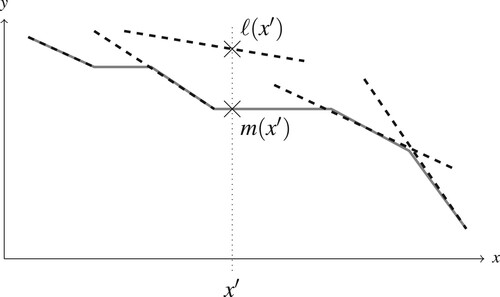
Figure 5 shows an example of the monotone lower envelope. Our approximation quality measures are invariant under taking the monotone lower envelope since it corresponds to the addition of the ordering cone ${\mathbb{R}}_{\ge 0}^K$.

Figure 5. Illustration of the monotone lower envelope m (solid line) for a set of segments (dashed). The dotted line shows the difference in value for the monotone lower envelope m and the standard lower envelope ℓ at the position $x^{\prime }$.

Proposition 3.2

Invariance of measures under monotone lower envelope

Let $A=\bigcup _{i=1}^n{s}_i$ be an approximation consisting of a set of segments $s_1,\dots s_n$. Let $A^{\prime }$ denote the monotone lower envelope of $s_1,\dots s_n$. Then the following equalities hold:

(1)	$N\left(A\right)=N\left(A^{\prime }\right)$
(2)	${\delta }_{\mathrm{vol}}(Z,A)={\delta }_{\mathrm{vol}}(Z,A^{\prime })$
(3)	${ϵ}_d\left(A\right)={ϵ}_d\left(A^{\prime }\right)$

A proof is provided in Appendix 1. The result shows that we can work with the monotone lower envelope without affecting our guarantees on the approximation quality.

Complexity of monotone lower envelopes

For our convergence guarantees, we need a bound on the number of segments contained in the monotone lower envelope.

We denote the standard lower envelope complexity, i.e. the maximal number of segments occurring in the lower envelope of n segments in the plane, by $\lambda \left(n\right)$. The following classic bound from computational geometry limits this standard lower envelope complexity to an almost-linear growth.

Lemma 3.1

[35,36]

For $n\in \mathbb{N}$ the standard lower envelope complexity is bounded by $\lambda \left(n\right)\le 2n(\ln (n)+1)$ and also by $\lambda \left(n\right)\le 52n\left(\alpha \right(n)+1)$ where α is the inverse Ackermann function, a very slowly growing function.

As a corollary, we obtain the following bound on the maximal number of segments in a monotone lower envelope which we denote by $\overline{\lambda }\left(n\right)$.

Corollary 3.1

Complexity of monotone lower envelopes

Let a set S of n line segments be given. Then the monotone lower envelope of these segments consists of at most $\overline{\lambda }\left(n\right)\le \lambda \left(2n\right)\le min\left\{4n\right(\ln \left(2n\right)+1),104n(\alpha \left(2n\right)+1\left)\right\}$ many segments.

Proof.

We can obtain the monotone lower envelope in the following way: We add for each segment $s\in S$ an additional horizontal segment $s^{\prime }$ extending from the right endpoint of s until the largest x-coordinate in S. Let $S^{\prime }$ be this extended set of segments. Due to the extensions with the horizontal segments, the lower envelope of $S^{\prime }$ is equal to the monotone lower envelope of S. The number of segments of the monotone lower envelope of S is thus bounded by the number of segments in the standard lower envelope of $S^{\prime }$. Since $|S^{\prime }|\le 2|S|$ we thus obtain from applying Lemma 3.1 on $S^{\prime }$ the upper bound $\overline{\lambda }\left(n\right)\le \lambda \left(|S^{\prime }|\right)\le \lambda \left(2|S|\right)\le min\left\{4n\right(\ln \left(2n\right)+1),104n(\alpha \left(2n\right)+1\left)\right\}$ for the number of segments in the monotone lower envelope.

Note that both functions $\lambda \left(n\right)$ and $\overline{\lambda }\left(n\right)$ are monotonically increasing since by adding a small segment at an appropriate place the number of segments in the lower envelope can always be increased.

3.3. Convergence bound

Using monotone lower envelopes, we now show that the Adaptive Patch Approximation Algorithm 1 achieves a convergence with respect to the difference volume which is only a small factor away from the theoretical optimum given by the patch complexity.

Lemma 3.2

Consequence of Improvement guarantee

Let Z be the set of all attainable objective vectors and $A\subseteq Z$ the current approximation. Suppose that we generate the next approximation $A^{\prime }$ by adding a segment patch fulfilling the Integrated improvement guarantee with level $\kappa >0$. Then, the new difference volume ${\delta }_{\mathrm{vol}}(Z,A^{\prime })$ is bounded by ${\delta }_{\mathrm{vol}}(Z,A^{\prime })\le {\delta }_{\mathrm{vol}}(Z,A)\left(1-\frac{\kappa }{2\overline{\lambda }\left(N_{{\delta }_{\mathrm{vol}}}^{\mathrm{S}}\left({\delta }_{\mathrm{vol}}\right(Z,A\left)/2\right)\right)}\right).$

Proof.

We show the statement by establishing the bound (4) ${\delta }_{\mathrm{vol}}(Z,A^{\prime })\le {\delta }_{\mathrm{vol}}(Z,A)-\kappa \frac{{\delta }_{\mathrm{vol}}(Z,A)-ϵ}{\overline{\lambda }\left(N_{{\delta }_{\mathrm{vol}}}^{\mathrm{S}}\right(ϵ\left)\right)}\mathrm{f}\mathrm{o}\mathrm{r}\mathrm{a}\mathrm{l}\mathrm{l}ϵ>0.$(4) The claim of the lemma then follows from plugging in $ϵ={\delta }_{\mathrm{vol}}(Z,A)/2$.

For $ϵ\ge {\delta }_{\mathrm{vol}}(Z,A)$ the bound (4(4) ${\delta }_{\mathrm{vol}}(Z,A^{\prime })\le {\delta }_{\mathrm{vol}}(Z,A)-\kappa \frac{{\delta }_{\mathrm{vol}}(Z,A)-ϵ}{\overline{\lambda }\left(N_{{\delta }_{\mathrm{vol}}}^{\mathrm{S}}\right(ϵ\left)\right)}\mathrm{f}\mathrm{o}\mathrm{r}\mathrm{a}\mathrm{l}\mathrm{l}ϵ>0.$(4) ) follows immediately, since ${\delta }_{\mathrm{vol}}(Z,A^{\prime })\le {\delta }_{\mathrm{vol}}(Z,A)$ holds due to the monotonicity of the difference volume.

Let some $ϵ<{\delta }_{\mathrm{vol}}(Z,A)$ be given. By the definition of the segment patch complexity $N_{{\delta }_{\mathrm{vol}}}^{\mathrm{S}}\left(ϵ\right)$ there exists a set $S^{\ast }$ of $|S^{\ast }|=N_{{\delta }_{\mathrm{vol}}}^{\mathrm{S}}\left(ϵ\right)$ many segment patches such that ${\delta }_{\mathrm{vol}}(Z,S^{\ast })\le ϵ$. Let $S^{\prime }$ be the monotone lower envelope of $S^{\ast }$. It holds ${\delta }_{\mathrm{vol}}(Z,S^{\prime })={\delta }_{\mathrm{vol}}(Z,S^{\ast })$ by Proposition 3.2. Because $S^{\prime }$ is a monotone lower envelope, the segments of $S^{\prime }$ cover the whole range $[0,1]$ on the x-axis without overlapping. We can thus represent the difference volume ${\delta }_{\mathrm{vol}}(Z,S^{\ast })\le ϵ$ as ${\delta }_{\mathrm{vol}}(Z,S^{\ast })={\delta }_{\mathrm{vol}}(Z,S^{\prime })=\sum _{\mathrm{s}\mathrm{e}\mathrm{g}\mathrm{m}\mathrm{e}\mathrm{n}\mathrm{t}{s}^{\prime }\mathrm{i}\mathrm{n}{S}^{\prime }}{\int }_{X_1\left(s^{\prime }\right)}^{X_2\left(s^{\prime }\right)}\left(s_y^{\prime }\left(x\right)-Z_y\left(x\right)\right)\mathrm{d}x$ using the representation (3(3) $\begin{array}{rl}{\delta }_{\mathrm{vol}}(Z,A)& =\mathrm{vol}\left(\left(\left(Z+{\mathbb{R}}_{\ge 0}^2\right)\setminus \left(A+{\mathbb{R}}_{\ge 0}^2\right)\right)\cap [0,1{]}^2\right)\\ & ={\int }_0^1{\int }_0^1{\mathbf{1}}_{\left(Z+{\mathbb{R}}_{\ge 0}^2\right)\setminus \left(A+{\mathbb{R}}_{\ge 0}^2\right)}(x,y)\mathrm{d}x\mathrm{d}y\\ & ={\int }_0^1\left({\int }_0^1{\mathbf{1}}_{\left(Z+{\mathbb{R}}_{\ge 0}^2\right)\setminus \left(A+{\mathbb{R}}_{\ge 0}^2\right)}(x,y)\mathrm{d}y\right)\mathrm{d}x\\ & ={\int }_0^1\left(A_y\right(x)-Z_y(x\left)\right)\mathrm{d}x.\end{array}$(3) ) by a comparison to the true Pareto frontier given by Z. Using the same partition of the x-axis given by these segments, we can represent the current difference volume as ${\delta }_{\mathrm{vol}}(Z,A)=\sum _{\mathrm{s}\mathrm{e}\mathrm{g}\mathrm{m}\mathrm{e}\mathrm{n}\mathrm{t}{s}^{\prime }\mathrm{i}\mathrm{n}{S}^{\prime }}{\int }_{X_1\left(s\right)}^{X_2\left(s^{\prime }\right)}\left(A_y\left(x\right)-Z_y\left(x\right)\right)\mathrm{d}x.$ By taking the difference of the integrals, we arrive at the inequality $\begin{array}{rl}{\delta }_{\mathrm{vol}}(Z,A)-ϵ& \le {\delta }_{\mathrm{vol}}(Z,A)-{\delta }_{\mathrm{vol}}(Z,S^{\ast })\\ & =\sum _{\mathrm{s}\mathrm{e}\mathrm{g}\mathrm{m}\mathrm{e}\mathrm{n}\mathrm{t}{s}^{\prime }\mathrm{i}\mathrm{n}{S}^{\prime }}{\int }_{X_1\left(s^{\prime }\right)}^{X_2\left(s^{\prime }\right)}\left(A_y\left(x\right)-s_y^{\prime }\left(x\right)\right)\mathrm{d}x.\end{array}$ Since $ϵ<{\delta }_{\mathrm{vol}}(Z,A)$ holds and because for at least one of the summands a value not smaller than the average value must occur, there exists a segment $s^{\ast }\in S^{\prime }$ that fulfils the inequality $I_A\left(s^{\ast }\right)={\int }_{X_1\left(s^{\ast }\right)}^{X_2\left(s^{\ast }\right)}\left(A_y\left(x\right)-s_y^{\ast }\left(x\right)\right)\mathrm{d}x\ge \frac{1}{|S^{\prime }|}\left({\delta }_{\mathrm{vol}}(Z,A)-ϵ\right).$ Let s be the new segment patch added to the approximation. Since s fulfils the Integrated improvement guarantee, the improvement obtained by s is at least within a factor κ of that obtained by $s^{\ast }$. Thus we have $I_A\left(s\right)\ge \kappa I_A\left(s^{\ast }\right)\ge \frac{\kappa }{|S^{\prime }|}\left({\delta }_{\mathrm{vol}}(Z,A)-ϵ\right)\ge \frac{\kappa }{\overline{\lambda }\left(N_{{\delta }_{\mathrm{vol}}}^{\mathrm{S}}\right(ϵ\left)\right)}\left({\delta }_{\mathrm{vol}}(Z,A)-ϵ\right)$ where we used the fact that the set $S^{\prime }$ contains at most $|S^{\prime }|\le \overline{\lambda }\left(N_{{\delta }_{\mathrm{vol}}}^{\mathrm{S}}\right(ϵ\left)\right)$ many segments.

According to Proposition 3.1 by adding the segment patch s, the difference volume ${\delta }_{\mathrm{vol}}$ decreases by at least $I_A\left(s\right)$. We thus obtain the statement (4(4) ${\delta }_{\mathrm{vol}}(Z,A^{\prime })\le {\delta }_{\mathrm{vol}}(Z,A)-\kappa \frac{{\delta }_{\mathrm{vol}}(Z,A)-ϵ}{\overline{\lambda }\left(N_{{\delta }_{\mathrm{vol}}}^{\mathrm{S}}\right(ϵ\left)\right)}\mathrm{f}\mathrm{o}\mathrm{r}\mathrm{a}\mathrm{l}\mathrm{l}ϵ>0.$(4) ) by using the bound on $I_A\left(s\right)$.

We are now able to show the main convergence result of our algorithm: The number of iterations required to reach a difference volume of ε is close to the theoretical optimum $N_{{\delta }_{\mathrm{vol}}}^{\mathrm{S}}\left(ϵ\right)$.

Theorem 3.1

Convergence of the Adaptive Patch Approximation Algorithm

Let $ϵ\in (0,1)$ be an arbitrary bound on the difference volume. Then, the approximation returned by the Adaptive Patch Approximation Algorithm 1 reaches a difference volume of at most ε after at most $\frac{2}{\kappa }\overline{\lambda }\left(N_{{\delta }_{\mathrm{vol}}}^{\mathrm{S}}\left(ϵ/2\right)\right)\ln \left(1/ϵ\right)$ many iterations.

Proof.

Let $A_0,A_1,\dots$ be the sequence of approximations generated by the iterations of the algorithm, where $A_0$ is the start approximation. Let $k\in \mathbb{N}$ be an index for which ${\delta }_{\mathrm{vol}}(Z,A_k)>ϵ/2$ holds. Since the patch complexity is a monotonically decreasing function, this implies $N_{{\delta }_{\mathrm{vol}}}^{\mathrm{S}}\left({\delta }_{\mathrm{vol}}\right(Z,A_{\ell }\left)/2\right)\le N_{{\delta }_{\mathrm{vol}}}^{\mathrm{S}}\left(ϵ/2\right)\mathrm{f}\mathrm{o}\mathrm{r}\mathrm{a}\mathrm{l}\mathrm{l}\ell \in \{0,\dots ,k\}.$ Lemma 3.2 hence yields for each iteration $\ell \in \{0,\dots ,k\}$ the following bound for the improvement $\begin{array}{rl}{\delta }_{\mathrm{vol}}(Z,A_{\ell +1})& \le {\delta }_{\mathrm{vol}}(Z,A_{\ell })\left(1-\frac{\kappa }{2\overline{\lambda }\left(N_{{\delta }_{\mathrm{vol}}}^{\mathrm{S}}\left({\delta }_{\mathrm{vol}}\right(Z,A_{\ell }\left)/2\right)\right)}\right)\\ & \le {\delta }_{\mathrm{vol}}(Z,A_{\ell })\left(1-\frac{\kappa }{2\overline{\lambda }\left(N_{{\delta }_{\mathrm{vol}}}^{\mathrm{S}}\left(ϵ/2\right)\right)}\right).\end{array}$ As ${\delta }_{\mathrm{vol}}(Z,A_0)\le 1$ by the definition of the difference volume, we obtain the total bound ${\delta }_{\mathrm{vol}}(Z,A_k)\le {\left(1-\frac{\kappa }{2\overline{\lambda }\left(N_{{\delta }_{\mathrm{vol}}}^{\mathrm{S}}\left(ϵ/2\right)\right)}\right)}^k.$ Thus, to achieve ${\delta }_{\mathrm{vol}}(Z,A_k)\le ϵ$, at most $k\le \ln \left(ϵ\right)\cdot {\left(\ln \left(1-\frac{\kappa }{2\overline{\lambda }\left(N_{{\delta }_{\mathrm{vol}}}^{\mathrm{S}}\left(ϵ/2\right)\right)}\right)\right)}^{-1}$ many iterations are needed. By using the inequality $\ln (1-x)\le -x$ for $x<1$ which implies $(\ln (1-x){)}^{-1}\ge (-x{)}^{-1}$, we obtain from above $k\le \ln \left(ϵ\right)\cdot {\left(-\frac{\kappa }{2\overline{\lambda }\left(N_{{\delta }_{\mathrm{vol}}}^{\mathrm{S}}\left(ϵ/2\right)\right)}\right)}^{-1}=2\ln \left(1/ϵ\right)\frac{\overline{\lambda }\left(N_{{\delta }_{\mathrm{vol}}}^{\mathrm{S}}\left(ϵ/2\right)\right)}{\kappa }$ as claimed, where we used $\ln \left(ϵ\right)<\ln \left(1\right)=0$.

4. Efficiently computing segment patches

In the preceding section, we have shown that the Adaptive Patch Approximation Algorithm 1 achieves a near-optimal convergence with respect to the number of iterations. In this section, we describe how the individual iterations can be implemented. The key task here is to develop an algorithm that efficiently finds a good segment patch. In particular, we have to ensure that the improvement guarantee of Definition 3.2 is fulfilled without requiring too many optimizations of the underlying mixed-integer program.

Since we build our approximation A out of segment patches, the approximation can be described by the monotone lower envelope of the set of segment patches. We partition the objective space along the axis of the first objective $f_1$ according to these segments in the monotone lower envelope. In the following, we identify the x-axis with the value of the first objective function $f_1$. In this way, vertical regions are created. Figure 6 illustrates this partition of the objective space.

Figure 6. Illustration of the partition of objective space into regions induced by the segments of the approximation.

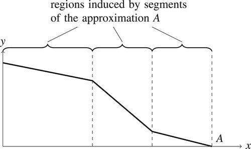
Our strategy for obtaining good segment patches is based on searching for segment patches that are fully contained in one of the regions induced by the monotone lower envelope of the approximation. When searching a segment patch $s^{\prime }$ with respect to segment s, we require that the bounds on the x-coordinates of the endpoints $X_1\left(s\right)\le X_1\left(s^{\prime }\right)\le X_2\left(s^{\prime }\right)\le X_2\left(s\right)$ are fulfilled. The restriction to such a region ensures that the approximation is linear with respect to x which enables a simple formulation of the desired optimization goal. We can reuse most found patches, only for segments that are new in the monotone lower envelope a new patch needs to be computed. In each iteration, we then add the patch that achieves the maximal improvement in difference volume among all candidate patches.

The realization of our Adaptive Patch Approximation algorithm can be summarized as follows in Main Algorithm 2. As a step to ensure approximate optimality in each iteration, we use Algorithm 3 which is described later.

Number of segment patch computations per iteration. In each iteration of the algorithm, the monotone lower envelope M of A has to be updated after the insertion of a new segment patch. However, we show that the number of changed segments in M is at most 4 per iteration. This follows from the fact that we add only segment patches to the approximation that have been contained in a region given by a previous segment. Thus, when adding a new segment patch p inside the region given by the old segment m from the monotone lower envelope, only two cases can occur which are also illustrated in Figure 7.

Figure 7. A new segment patch p (dotted) is found w.r.t. the reference segment m. Two cases can arise when the new patch p is inserted into the old monotone lower envelope (solid). In both cases, only four segments are updated or newly created in the new monotone lower envelope (dashed). (a) New segment above reference segment. (b) New segment below reference segment.

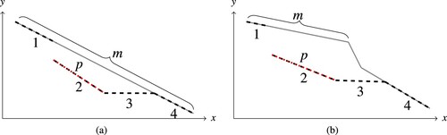
1. The new segment patch p is above the right endpoint of the segment m, i.e. has a larger y-coordinate everywhere. Then, at most four new segments can appear in the monotone lower envelope: A part of p, two parts of m (one the left and one to the right of p) and a horizontal segment.

2. The new segment p is (at least partially) below the right endpoint of m. Then, there is only one part of m and one part of p that might change. Additionally, only the horizontal segment extending from the right endpoint of p and the segment intersecting this horizontal segment can be created or updated. Thus, at most four segments are updated. There might, however, be segments from the monotone lower envelope that will be completely removed by the insertion of p.

Our discussion shows that at most 4 segments are updated in the monotone lower envelope per iteration. This results in the following bound on the effort required by Algorithm 2.

Proposition 4.1

Complexity of the Adaptive Patch Approximation Algorithm

The Adaptive Patch Approximation Algorithm 2 needs to compute at most 4 segment patches per iteration.

In the remainder of this section, we show the following statement that establishes the effectiveness and efficiency of Algorithm 2.

Theorem 4.1

The Adaptive Patch Approximation Algorithm 1 has the following properties for every fixed value of the parameter $0<\text{β}<1:$

(1)

A segment patch can be found by performing a single-objective optimization of two feasible points over the original feasibility set X of (1(1) $X=\left\{(c,d)\in {\mathbb{R}}^k\times {\mathbb{Z}}^m\mid g_i(c,d)\le 0\mathrm{f}\mathrm{o}\mathrm{r}\mathrm{e}\mathrm{a}\mathrm{c}\mathrm{h}i\in I\right\}$(1) ) with additional linking constraints. This single-objective MIP has a linear objective and duplicates the constraints and continuous variables of (1(1) $X=\left\{(c,d)\in {\mathbb{R}}^k\times {\mathbb{Z}}^m\mid g_i(c,d)\le 0\mathrm{f}\mathrm{o}\mathrm{r}\mathrm{e}\mathrm{a}\mathrm{c}\mathrm{h}i\in I\right\}$(1) ), with an additional constant number of constraints and variables.

(2)

The patch improvement guarantee is always fulfilled with $\kappa =\frac{1}{8}(1-\text{β})$.

To prove this theorem, we perform a detailed analysis of the various steps of the algorithm.

4.1. Finding good segment patches by maximizing the Integrated improvement

In the Adaptive Patch Approximation algorithm, we need to find segment patches with maximal Integrated improvement with respect to the current segments. We now give an efficient MIP formulation for this task.

Expression for the Integrated improvement

The basis of our formulation is a simple expression for the Integrated improvement w.r.t. a single segment. Assume that the new segment patch $s^{\prime }$ is found inside the region induced by the segment s of the current monotone lower envelope, i.e. it holds $X_1\left(s\right)\le X_1\left(s^{\prime }\right)\le X_2\left(s^{\prime }\right)\le X_2\left(s\right)$. The Integrated improvement $I_s\left(s^{\prime }\right)$ can then be simplified to (5) $\begin{array}{rl}{I}_s\left(s^{\prime }\right)& ={\int }_{X_1\left(s^{\prime }\right)}^{X_2\left(s^{\prime }\right)}\left(s_y\right(x)-s_y^{\prime }(x\left)\right)\mathrm{d}x\\ & =\left(X_2\left(s^{\prime }\right)-X_1\left(s^{\prime }\right)\right)\\ & \cdot \left(Y_1\left(s\right)+\left(Y_2\right(s)-Y_1(s\left)\right)\frac{X_1\left(s^{\prime }\right)/2+X_2\left(s^{\prime }\right)/2-X_1\left(s\right)}{X_2\left(s\right)-X_1\left(s\right)}-\frac{Y_1\left(s^{\prime }\right)+Y_2\left(s^{\prime }\right)}{2}\right)\end{array}$(5) by using the linearity of the segments s and $s^{\prime }$.

Formulation of the MIP

Our implementation of the Adaptive Patch Approximation Algorihtm 1 is based on computing, with respect to each segment of the monotone lower envelope, a segment patch with approximately maximal Integrated improvement. We now show how such an optimization can be formulated in practice. For this, an approximately optimal solution is sufficient. We will show that we can obtain an approximation with a constant relative error that can be chosen to be as close to 0 as wanted.

To maximize the Integrated improvement corresponding to the reference segment s, we have to solve the following optimization problem. $\begin{array}{rl}& max{I}_s\left(s^{\ast }\right)\\ \mathrm{s}.\mathrm{t}.& s^{\ast }\mathrm{i}\mathrm{s}\mathrm{a}\mathrm{s}\mathrm{e}\mathrm{g}\mathrm{m}\mathrm{e}\mathrm{n}\mathrm{t}\mathrm{p}\mathrm{a}\mathrm{t}\mathrm{c}\mathrm{h}\mathrm{i}\mathrm{n}\mathrm{o}\mathrm{b}\mathrm{j}\mathrm{e}\mathrm{c}\mathrm{t}\mathrm{i}\mathrm{v}\mathrm{e}\mathrm{s}\mathrm{p}\mathrm{a}\mathrm{c}\mathrm{e}\\ & \begin{array}{c}{X}_2\left(s^{\ast }\right)\ge X_1\left(s^{\ast }\right)\\ X_1\left(s^{\ast }\right)\ge X_1\left(s\right)\\ X_2\left(s^{\ast }\right)\le X_2\left(s\right)\end{array}\end{array}$ We use here Definition 2.1 of segment patches in objective space. Note that according to this definition an extension in direction of the ordering cone is allowed and thus horizontal segment patches can also be considered. The requirement that $s^{\ast }$ is a segment patch can be explicitly modelled using linear inequalities and variables and constraints from the original mixed-integer program. By additionally using the expression (5(5) $\begin{array}{rl}{I}_s\left(s^{\prime }\right)& ={\int }_{X_1\left(s^{\prime }\right)}^{X_2\left(s^{\prime }\right)}\left(s_y\right(x)-s_y^{\prime }(x\left)\right)\mathrm{d}x\\ & =\left(X_2\left(s^{\prime }\right)-X_1\left(s^{\prime }\right)\right)\\ & \cdot \left(Y_1\left(s\right)+\left(Y_2\right(s)-Y_1(s\left)\right)\frac{X_1\left(s^{\prime }\right)/2+X_2\left(s^{\prime }\right)/2-X_1\left(s\right)}{X_2\left(s\right)-X_1\left(s\right)}-\frac{Y_1\left(s^{\prime }\right)+Y_2\left(s^{\prime }\right)}{2}\right)\end{array}$(5) ) for the Integrated improvement $I_s\left(s^{\ast }\right)$ we arrive at the following formulation (6(6) $\begin{array}{rl}(x_2-x_1)& \cdot \left(Y_1\left(s\right)+\left(Y_2\right(s)-Y_1(s\left)\right)\frac{x_1/2+x_2/2-X_1\left(s\right)}{X_2\left(s\right)-X_1\left(s\right)}-\frac{y_1+y_2}{2}\right)\end{array}$(6) ) to compute an optimal segment patch with endpoints $(x_1,y_1)$ and $(x_2,y_2)$. (6) $\begin{array}{rl}(x_2-x_1)& \cdot \left(Y_1\left(s\right)+\left(Y_2\right(s)-Y_1(s\left)\right)\frac{x_1/2+x_2/2-X_1\left(s\right)}{X_2\left(s\right)-X_1\left(s\right)}-\frac{y_1+y_2}{2}\right)\end{array}$(6) (7) $\begin{array}{rl}& \begin{array}{c}\mathrm{s}.\mathrm{t}.(c_1,d)\in X\\ (c_2,d)\in X\\ x_1\ge f_1(c_1,d)\\ x_2\ge f_1(c_2,d)\\ y_1\ge f_2(c_1,d)\\ y_2\ge f_2(c_2,d)\\ x_1\ge X_1\left(s\right)\\ x_2\le X_2\left(s\right)\\ x_1\le x_2\end{array}\end{array}$(7) The constraints $(c_1,d)\in X$ and $(c_2,d)\in X$ can be expressed by using the constraints of the original MIP. This requires at most twice the number of constraints and twice the number of continuous variables as in the original MIP. Note that every optimal solution fulfils $y_1=f_2(c,d)$ and $y_2=f_2(c,d)$ since $y_1$ and $y_2$ appear with a negative factor in the objective function.

Linearization of the objective function

The optimization objective in (6(6) $\begin{array}{rl}(x_2-x_1)& \cdot \left(Y_1\left(s\right)+\left(Y_2\right(s)-Y_1(s\left)\right)\frac{x_1/2+x_2/2-X_1\left(s\right)}{X_2\left(s\right)-X_1\left(s\right)}-\frac{y_1+y_2}{2}\right)\end{array}$(6) ) is nonlinear. To maintain the linear structure of the original MIP, we now linearize this objective. Using the linear substitutions $x=(x_2-x_1)$ and $y=Y_1\left(s\right)+\left(Y_2\right(s)-Y_1(s\left)\right)\frac{x_1/2+x_2/2-X_1\left(s\right)}{X_2\left(s\right)-X_1\left(s\right)}-\frac{y_1+y_2}{2}$ we obtain the following simple bilinear term for $I_s\left(s^{\prime }\right)$ which is identical to (6(6) $\begin{array}{rl}(x_2-x_1)& \cdot \left(Y_1\left(s\right)+\left(Y_2\right(s)-Y_1(s\left)\right)\frac{x_1/2+x_2/2-X_1\left(s\right)}{X_2\left(s\right)-X_1\left(s\right)}-\frac{y_1+y_2}{2}\right)\end{array}$(6) ) $I_s\left(s^{\prime }\right)=g(x,y):=x\cdot y.$ For this function g we perform now an approximate linearization. Note that by definition $x=x_2-x_1\ge 0$ is non-negative. Since the maximal value of $I_s\left(s^{\ast }\right)$ is at least 0 we can assume $y\ge 0$ and include it as a constraint in the problem. We thus only need to approximate the function g in the non-negative orthant. Due to the scaling of the objective vectors to $[0,1{]}^2$, we also know that the x- and y-value can be at most 1. Thus, approximating g in the square $[0,1{]}^2$ is sufficient. We use an approach based on the identity $g(x,y)=x\cdot y=\exp (\ln (x)+\ln (y\left)\right).$ Since $\exp$ is a monotone function, maximizing g is equivalent to maximizing $\ln \left(x\right)+\ln \left(y\right)$. For the logarithm we can give an upper approximation with linear inequalities based on tangents, since the logarithm is a concave function.

Approximation of the logarithm with linear inequalities

To provide a linearization of the Integrated improvement obtained by a segment patch, we give an approximation of $\ln \left(x\right)$ for values $x\in [{\delta }_0,1]$ larger than some constant threshold ${\delta }_0>0$. It is sufficient to restrict the approximation to this range, because smaller values of x correspond to an Integrated improvement which is guaranteed to be smaller than available alternatives. Our approach is based on tangents with an exponentially scaled discretization.

A similar problem of approximating a convex function via a convex piecewise linear approximation was considered in [37]. For the function $\ln (1+{\mathrm{e}}^x)$ it was shown that there is an optimal approximation consisting of tangents at appropriate breakpoints which can be found with an algorithm. We describe here a similar procedure, which given some prescribed additive accuracy ${\text{β}}^{\prime }>0$ finds a concave piecewise linear approximation of $\ln \left(x\right)$ with a minimal number of pieces.

Formally, we search a set of k lines described by the slope $a_i\in \mathbb{R}$ and y-intercept $b_i\in \mathbb{R}$ for $i=1,\dots ,k$, such that $\underset{i=1,\dots ,k}{min}{a}_{i}x+b_i-{\text{β}}^{\prime }\le \ln \left(x\right)\le \underset{i=1,\dots ,k}{min}{a}_{i}x+b_i\mathrm{f}\mathrm{o}\mathrm{r}\mathrm{a}\mathrm{l}\mathrm{l}x\in [{\delta }_0,1].$ This form allows us to later transform a maximization of $\ln \left(x\right)+\ln \left(y\right)$ into the approximately equivalent problem $\begin{array}{rl}& max{z}_x+z_y\\ \mathrm{s}.\mathrm{t}.& z_x\le a_{i}x+b_i\mathrm{f}\mathrm{o}\mathrm{r}\mathrm{e}\mathrm{a}\mathrm{c}\mathrm{h}i\in \{1,\dots ,k\}\\ & z_y\le a_{i}y+b_i\mathrm{f}\mathrm{o}\mathrm{r}\mathrm{e}\mathrm{a}\mathrm{c}\mathrm{h}i\in \{1,\dots ,k\},\end{array}$ with a linear structure. The approximation of $\ln \left(x\right)$ and correspondingly $\ln \left(y\right)$ within an additive error of ${\text{β}}^{\prime }$ yields a total relative error for the approximation of $x\cdot y$ of $\text{β}=1-\exp (-2{\text{β}}^{\prime })\in (0,1)$ as a simple calculation shows. With our construction we will establish the following statement.

Lemma 4.1

Approximation of the logarithm with linear inequalities

Let ${\text{β}}^{\prime }>0$ and ${\delta }_0>0$ be given. Then, there exists a set of lines of size $k\le \frac{\ln \left(1/{\delta }_0\right)}{\ln (1+\sqrt{2{\text{β}}^{\prime }})}$ which are given by the slopes $a_i\in \mathbb{R}$ and y-intercepts $b_i\in \mathbb{R}$, $i=1,\dots ,k$, such that $\underset{i=1,\dots ,k}{min}{a}_{i}x+b_i-{\text{β}}^{\prime }\le \ln \left(x\right)\le \underset{i=1,\dots ,k}{min}{a}_{i}x+b_i\mathrm{f}\mathrm{o}\mathrm{r}\mathrm{a}\mathrm{l}\mathrm{l}x\in [{\delta }_0,1].$

This lemma implies immediately, by replacing the value $b_i$ by $b_i+{\text{β}}^{\prime }$, that we can also obtain the similar approximation from below $\underset{i=1,\dots ,k}{min}{a}_{i}x+b_i\le \ln \left(x\right)\le \underset{i=1,\dots ,k}{min}{a}_{i}x+b_i+{\text{β}}^{\prime }\mathrm{f}\mathrm{o}\mathrm{r}\mathrm{a}\mathrm{l}\mathrm{l}x\in [{\delta }_0,1].$ The construction is based on the idea that each line of the approximation should be a tangent to $\ln \left(x\right)$. Choosing tangents is optimal, since any approximation that is not directly touching the graph of the logarithm can be improved by shifting and secants are not allowed because we want to overestimate the function $\ln \left(x\right)$.

In Appendix 2 the construction is described in detail and a proof of Lemma 4.1 is provided. Figure 8 shows the corresponding approximation for the case ${\text{β}}^{\prime }=0.2$ and ${\delta }_0=0.022$.

Figure 8. Approximation of the logarithm (solid line) via linear inequalities (dashed lines). The shown plot corresponds to the choice ${\text{β}}^{\prime }=0.2$. With the tangents through the three points $x_0$, $x_1$, $x_2$ we obtain an upper approximation of $\ln \left(x\right)$ with an additive error of at most ${\text{β}}^{\prime }=0.2$ for the interval $[{\delta }_0,1]=[z_3,1]\approx [0.022,1]$ which is attained at the points $z_1$, $z_2$ and $z_3$.

4.2. Establishing optimality of the algorithm

We show now that the Adaptive Patch Approximation Algorithm 2 fulfils the Integrated improvement guarantee with a factor of $\kappa =\frac{1}{8}(1-\text{β})$. This result then implies the almost-optimal convergence rate of the algorithm by Theorem 3.1. To establish the Integrated improvement guarantee, we have to show that the segment patch chosen by our algorithm obtains an Integrated improvement that is at least $\frac{1}{8}(1-\text{β})$ as large as the maximally possible Integrated improvement for an arbitrary segment patch. Our proof for this is based on the decomposition of the Integrated improvement obtained by the optimal segment patch into the regions given by the monotone lower envelope. We bound the number of regions for which a positive Integrated improvement occurs.

Notation for segment relations

New segment patches are found by optimizing with respect to given segments of the monotone lower envelope. The tree-like relations between these segments are the basis of our analysis. We denote the parent-segment of a segment patch p by $\mathrm{par}\left(p\right)$, which represents the segment m in which region the segment patch p was found by Algorithm 2. The set of parent-segments of an approximation A consists of the parent-segments of each of the segment patches in A. The children of a segment m are the segments that were added to the monotone lower envelope by Algorithm 2 as a result of the optimization within the segment m. The set of children of m is denoted by $\mathrm{chldn}\left(m\right)$. As shown in the discussion of Proposition 4.1, the number of children of a segment is at most 4.

Local optimality guarantee

Due to the linearization, we obtain only segment patches that maximize within a factor of $(1-\text{β})$ the Integrated improvement possible inside a region. Thus, we cannot directly guarantee exact optimality, which is required for our decomposition approach. We can use instead the following local guarantee which is simpler to ensure.

Definition 4.1

Local optimality guarantee

Let $s^{\ast }$ be a new segment patch that was returned by the algorithm and $\mathrm{par}\left(s^{\ast }\right)$ its corresponding parent segment. The segment patch $s^{\ast }$ fulfils the local optimality guarantee if for every other segment patch $s^{\prime }$ with range $\left[X_1\right(s^{\prime }),X_2(s^{\prime }\left)\right]=\left[X_1\right(\mathrm{par}\left(s^{\ast }\right)),X_2(\mathrm{par}\left(s^{\ast }\right)\left)\right]$ the Integrated improvement is not larger, i.e. $I_{\mathrm{par}\left(s^{\ast }\right)}\left(s^{\prime }\right)\le I_{\mathrm{par}\left(s^{\ast }\right)}\left(s^{\ast }\right).$

As the guarantee only concerns fixed x-coordinates the Integrated improvement $I_{\mathrm{par}\left(s^{\ast }\right)}\left(s^{\prime }\right)$ becomes linear in the y-coordinates. Thus the guarantee can be easily provided as a post-optimization step by Algorithm 3.

As a consequence of the local optimality guarantee, we can rule out that a positive Integrated improvement is possible throughout the whole region of the parent segment. We use here the extended form ${\tilde{I}}_s\left(s^{\prime }\right)$ of the Integrated improvement of $s^{\prime }$ with respect to a segment s for the case that s does not cover the whole x-range of $s^{\prime }$. In this situation, the integral is restricted to the overlapping x-range between the segments as ${\tilde{I}}_s\left(s^{\prime }\right):={\int }_{max\left\{X_1\right(s),X_1(s^{\prime }\left)\right\}}^{min\left\{X_2\right(s),X_2(s^{\prime }\left)\right\}}\left(s_y\right(x)-s_y^{\prime }(x\left)\right)\mathrm{d}x.$ In the case that the segment $s^{\prime }$ is covered by the reference segment s, i.e. if $X_1\left(s\right)\le X_1\left(s^{\prime }\right)\le X_2\left(s^{\prime }\right)\le X_2\left(s\right)$ holds, this extended Integrated improvement is equivalent to the original ${\tilde{I}}_s\left(s^{\prime }\right)=I_s\left(s^{\prime }\right)$.

Lemma 4.2

No further improvement over the whole interval

Assume that the local optimality guarantee is fulfilled for $s^{\ast }$. Then, any new segment patch $s^{\prime }$ extending over the whole x-interval of $\mathrm{par}\left(s^{\ast }\right)$ $\left[X_1\right(s^{\prime }),X_2(s^{\prime }\left)\right]=\left[X_1\right(\mathrm{par}\left(s^{\ast }\right)),X_2(\mathrm{par}\left(s^{\ast }\right)\left)\right]$ does not obtain a positive Integrated improvement over this interval, i.e. $\sum _{s^{\circ }\in \mathrm{chldn}(\mathrm{par}(s^{\ast }\left)\right)}{\tilde{I}}_{s^{\circ }}\left(s^{\prime }\right)\le 0.$

Proof.

Let $s^{\prime }$ be any segment patch fulfilling the assumption. Since this segment patch extends over the whole region induced by $\mathrm{par}\left(s^{\ast }\right)$, the Integrated improvement of $s^{\prime }$ can be decomposed as $\begin{array}{rl}\sum _{s^{\circ }\in \mathrm{chldn}(\mathrm{par}(s^{\ast }\left)\right)}{\tilde{I}}_{s^{\circ }}\left(s^{\prime }\right)& ={\tilde{I}}_{\mathrm{par}\left(s^{\ast }\right)}\left(s^{\prime }\right)-\sum _{s^{\circ }\in \mathrm{chldn}(\mathrm{par}(s^{\ast }\left)\right)}{\tilde{I}}_{\mathrm{par}\left(s^{\ast }\right)}\left(s^{\circ }\right)\\ & \le {\tilde{I}}_{\mathrm{par}\left(s^{\ast }\right)}\left(s^{\ast }\right)-\sum _{s^{\circ }\in \mathrm{chldn}(\mathrm{par}(s^{\ast }\left)\right)}{\tilde{I}}_{\mathrm{par}\left(s^{\ast }\right)}\left(s^{\circ }\right)\\ & \le {\tilde{I}}_{\mathrm{par}\left(s^{\ast }\right)}\left(s^{\ast }\right)-{\tilde{I}}_{\mathrm{par}\left(s^{\ast }\right)}\left(s^{\ast }\right)=0,\end{array}$ where we used the local optimality guarantee for the first inequality and the fact that $s^{\ast }\in \mathrm{chldn}(\mathrm{par}(s^{\ast }\left)\right)$ is a child of $\mathrm{par}\left(s^{\ast }\right)$ for the second inequality.

Obtaining the Integrated improvement guarantee

The following decomposition of the Integrated improvement $I_A\left(s^{\prime }\right)$ of a an arbitrary segment patch shows that the best segment patch restricted to a region of the approximation obtains at least $\frac{1}{8}$ of that Integrated improvement. Thus searching for segment patches inside the individual regions will yield sufficiently good results.

Lemma 4.3

Separate optimization in each segment is sufficient

Let $s^{\prime }$ be an arbitrary segment patch. Assume that the local optimality guarantee holds for all segment patches created by the algorithm. Then it holds $I_A\left(s^{\prime }\right)\le max\left\{8\underset{s^{\circ }\in M}{max}{I}_{s^{\circ }}\left(s^{\prime }\right),0\right\},$ i.e. when restricting the optimization to regions of the monotone lower envelope, at least $\frac{1}{8}$ of the Integrated improvement is obtained.

Proof.

Consider the set S of parent-segments which regions intersect with that of $s^{\prime }$ given as $S=\left\{\mathrm{p}\mathrm{a}\mathrm{r}\mathrm{e}\mathrm{n}\mathrm{t}\text{-}\mathrm{s}\mathrm{e}\mathrm{g}\mathrm{m}\mathrm{e}\mathrm{n}\mathrm{t}s\mid \left[X_1\right(s),X_2(s\left)\right]\cap \left[X_1\right(s^{\prime }),X_2(s^{\prime }\left)\right]\ne set\right\}.$ Note that with respect to the children of all other parent-segments the Integrated improvement of $s^{\prime }$ is 0 by definition, since their intersection is empty. We partition the set S into the subsets $S_1$ and $S_2$ given as

• $S_1:=\{s\in S\mid [X_1\left(s\right),X_2\left(s\right)]\subseteq [X_1\left(s^{\prime }\right),X_2\left(s^{\prime }\right)\left]\right\},$

• $S_2:=S\setminus S_1.$

For parent-segments $s\in S_1$, we can restrict the segment patch $s^{\prime }$ to the interval $\left[X_1\right(s),X_2(s\left)\right]$ along the x-axis, since this interval is by definition fully contained in the interval corresponding to $s^{\prime }$. By Lemma 4.2 it then holds $\sum _{s^{\circ }\in \mathrm{chldn}\left(s\right)}{\tilde{I}}_{s^{\circ }}\left(s^{\prime }\right)\le 0.$ Thus, the contribution of the children of segments in $S_1$ to the whole Integrated improvement sum is nonpositive. There are at most two elements in $S_2$ since an interval has only two endpoints and the parent-segments are non-overlapping. These parent-segments have at most four children each, corresponding to eight segments in total. Combining the above observations, we obtain the following decomposition of the sum of Integrated improvement volumes which leads to the claim $\begin{array}{rl}{I}_A\left(s^{\prime }\right)& =\sum _{s^{\circ }\in M}{\tilde{I}}_{s^{\circ }}\left(s^{\prime }\right)\\ & =\sum _{s\in S}\sum _{s^{\circ }\in \mathrm{chldn}\left(s\right)}{\tilde{I}}_{s^{\circ }}\left(s^{\prime }\right)\\ & =\sum _{s\in S_1}\underset{\le 0}{\underbrace{\sum _{s^{\circ }\in \mathrm{chldn}\left(s\right)}{\tilde{I}}_{s^{\circ }}\left(s^{\prime }\right)}}+\underset{\le 8\mathrm{e}\mathrm{l}\mathrm{e}\mathrm{m}\mathrm{e}\mathrm{n}\mathrm{t}\mathrm{s}{\mathrm{s}}^{\circ }\mathrm{i}\mathrm{n}\mathrm{t}\mathrm{o}\mathrm{t}\mathrm{a}\mathrm{l}}{\underbrace{\sum _{s\in S_2}\sum _{s^{\circ }\in \mathrm{chldn}\left(s\right)}}}{\tilde{I}}_{s^{\circ }}\left(s^{\prime }\right)\\ & \le max\left\{8\underset{s\in S_2}{max}\underset{s^{\circ }\in \mathrm{chldn}\left(s\right)}{max}{\tilde{I}}_{s^{\circ }}\left(s^{\prime }\right),0\right\}\\ & \le max\left\{8\underset{s^{\circ }\in M}{max}{\tilde{I}}_{s^{\circ }}\left(s^{\prime }\right),0\right\}.\text{■}\end{array}$

As we have now shown that optimizing within the regions given by the segments of the monotone lower envelope is sufficient, we can obtain the Integrated improvement guarantee with a corresponding constant factor.

Theorem 4.2

Realization of the Integrated improvement guarantee

The Adaptive Patch Approximation Algorithm 2 fulfils the Integrated improvement guarantee of Definition 3.2 with $\kappa =\frac{1}{8}(1-\text{β})$. Here $1-\text{β}$ is the approximation factor for finding individual segment patches.

Proof.

Let A be the current approximation A generated by Algorithm 2 and M the corresponding monotone lower envelope. Let $s^{\ast }$ be an arbitrary segment patch. We have to show that the optimal segment patch $s^{\prime }$ found during the optimization within a region of M achieves an Integrated improvement $I_A\left(s^{\prime }\right)$ of at least a fraction $\kappa =\frac{1}{8}(1-\text{β})$ of the Integrated improvement $I_A\left(s^{\ast }\right)$ of $s^{\ast }$, i.e. we aim to show the inequality $I_A\left(s^{\prime }\right)\ge \frac{1}{8}(1-\text{β})I_A\left(s^{\ast }\right).$ Since Algorithm 2 ensures for all added segment patches that the local optimality guarantee is fulfilled, by using Algorithm 3 as a subroutine, we can apply Lemma 4.3 which yields the bound $I_A\left(s^{\ast }\right)\le max\left\{8\underset{s^{\circ }\in M}{max}{\tilde{I}}_{s^{\circ }}\left(s^{\ast }\right),0\right\}.$ In the case that $I_A\left(s^{\ast }\right)\le 0$ holds, the inequality $I_A\left(s^{\prime }\right)\ge \frac{1}{8}(1-\text{β})I_A\left(s^{\ast }\right)=0$ is fulfilled since the segment patch $s^{\prime }$ has a non-negative integrated improvement $I_A\left(s^{\prime }\right)\ge 0$. The nonnegativity of $I_A\left(s^{\prime }\right)$ is guaranteed since the segment patch of the last iteration would obtain again an improvement in the new iteration of 0 and the algorithm choose a segment patch $s^{\prime }$ with at least this integrated improvement.

We thus can assume $I_A\left(s^{\ast }\right)>0$ in the following. By the inequality above there exists a segment $s^{\circ }\in M$ in the monotone lower envelope M which fulfils ${\tilde{I}}_{s^{\circ }}\left(s^{\ast }\right)\ge \frac{1}{8}{I}_A\left(s^{\ast }\right).$ Since we perform an approximate optimization of the Integrated improvement, we also compute a segment patch s with (approximately) maximal Integrated improvement w.r.t. the segment $s^{\circ }$ of the monotone lower envelope. Since we have an approximation factor of $1-\text{β}$ for the individual optimization, it holds ${\tilde{I}}_{s^{\circ }}\left(s\right)\ge (1-\text{β}){\tilde{I}}_{s^{\circ }}\left(s^{\ast }\right).$ Because our algorithms outputs a segment patch $s^{\prime }$ with an Integrated improvement of at least ${\tilde{I}}_{s^{\circ }}\left(s\right)$ provided by the alternative patch s, we obtain $I_A\left(s^{\prime }\right)\ge {\tilde{I}}_{s^{\circ }}\left(s\right)\ge (1-\text{β}){\tilde{I}}_{s^{\circ }}\left(s^{\ast }\right)\ge \frac{1}{8}(1-\text{β})I_A\left(s^{\ast }\right).$ This implies that the Integrated improvement guarantee (Definition 3.2) is fulfilled with the factor $\kappa =\frac{1}{8}(1-\text{β})$.

The combination of this guarantee with our previous convergence analysis based on the Integrated improvement guarantee in Theorem 3.1 establishes that the Adaptive Patch Approximation Algorithm 2 computes approximations to the Pareto frontier with a convergence rate that almost matches the theoretical lower bound provided by the patch complexity.

Main theorem 4.1 (Performance of the Adaptive Patch Approximation Algorithm): The number of iterations of the Adaptive Patch Approximation Algorithm 2 for reaching a difference volume that is less or equal to ε is bounded in terms of the segment patch complexity $N_{{\delta }_{\mathrm{vol}}}^{\mathrm{S}}$ by $\frac{16}{1-\text{β}}\overline{\lambda }\left(N_{{\delta }_{\mathrm{vol}}}^{\mathrm{S}}\left(ϵ/2\right)\right)\ln \left(1/ϵ\right).$ The number of single-objective MIP optimizations performed by the algorithm is asymptotically bounded by the same quantity since per iteration at most 5 single-objective MIPs need to be solved.

Here $1-\text{β}$ is a constant factor given by the approximation factor with respect to optimal Integrated improvement. The function $\overline{\lambda }$ denotes the monotone lower envelope complexity, a function that has an almost linear growth rate.

Using the bounds on the monotone lower envelope complexity from Corollary 3.1, we obtain the alternative upper bounds on the number of iterations $64N_{{\delta }_{\mathrm{vol}}}^{\mathrm{S}}\left(ϵ/2\right)\left(\ln \left(2N_{{\delta }_{\mathrm{vol}}}^{\mathrm{S}}\left(ϵ/2\right)\right)+1\right)\frac{\ln \left(1/ϵ\right)}{1-\text{β}}$ and $1664N_{{\delta }_{\mathrm{vol}}}^{\mathrm{S}}\left(ϵ/2\right)\left(\alpha \left(2N_{{\delta }_{\mathrm{vol}}}^{\mathrm{S}}\left(ϵ/2\right)\right)+1\right)\frac{\ln \left(1/ϵ\right)}{1-\text{β}}.$

Remark 4.1

Near-optimality of the algorithm

Main theorem 4.1 shows that the algorithm is asymptotically almost optimal. By the definition of the segment patch complexity $N_{{\delta }_{\mathrm{vol}}}^{\mathrm{S}}$, to reach a difference volume of at most ε any algorithm needs to output at least $N_{{\delta }_{\mathrm{vol}}}^{\mathrm{S}}\left(ϵ\right)$ many segment patches. The factor in the algorithm is $N_{{\delta }_{\mathrm{vol}}}^{\mathrm{S}}\left(ϵ/2\right)$. Although this value can be slightly larger than the lower bound $N_{{\delta }_{\mathrm{vol}}}^{\mathrm{S}}\left(ϵ\right)$, it is typically only a small constant factor away from it.

The factor $\overline{\lambda }\left(N_{{\delta }_{\mathrm{vol}}}^{\mathrm{S}}\right(ϵ/2\left)\right)$ is necessary since our algorithm outputs a set of non-overlapping segment patches in the end. The smallest possible number of segment patches of an approximation of the Pareto frontier with difference volume at most ε is by definition $N_{{\delta }_{\mathrm{vol}}}^{\mathrm{S}}\left(ϵ\right)$. These segment patches can, however, be overlapping. To achieve the same small difference volume with non-overlapping segments, in the worst case $\overline{\lambda }\left(N_{{\delta }_{\mathrm{vol}}}^{\mathrm{S}}\right(ϵ\left)\right)$ many segments are needed. Thus our algorithm cannot be improved in this respect as long as it outputs non-overlapping segments patches.

The factor $\ln \left(1/ϵ\right)$ is coming from the fact that we do a greedy choice in each step that is only approximately optimal. Due to this property, a reduction of the difference volume by a constant factor can only be guaranteed after a number of patches proportional to $N_{{\delta }_{\mathrm{vol}}}^{\mathrm{S}}\left(ϵ\right)$ have been added. Hence, asymptotically at least $N_{{\delta }_{\mathrm{vol}}}^{\mathrm{S}}\left(ϵ\right)\ln \left(1/ϵ\right)$ many patches need to be added.

5. Numerical evaluation

Our algorithm is applicable to all types of bicriteria convex mixed-integer problems. This includes also linear and convex-quadratic problems. As there is a larger set of alternative methods available for the linear case, we perform a detailed comparison of the computational efficiency with other algorithms for this case in Subsection 5.4. The literature for the convex-quadratic and nonlinear convex case does not yet have a large number of available algorithms. We thus present the results on small-scale problems, focussing of illustrating the behaviour of our algorithm. In Subsection 5.2, we discuss a convex-quadratic problem, the Subsection 5.3 treats a nonlinear problem which is non-quadratic.

5.1. Computational configuration

In our implementation of the algorithm, we choose the sequence $x_0=\frac{1}{2},\frac{1}{4},\frac{1}{8},\dots$ as the touching points of the tangents of the approximation of the logarithm. The corresponding approximation error ${\text{β}}^{\prime }$ has the value ${\text{β}}^{\prime }=-\ln \left(1/2\right)-1-\ln (-\ln (1/2\left)\right)\approx 0.05966$. The corresponding relative error for optimizing the product is thus $\text{β}=1-\exp (-2{\text{β}}^{\prime })\approx 0.11247$. Our implementation hence fulfils by Theorem 4.2 the Integrated improvement guarantee with $\kappa =\frac{1}{8}(1-\text{β})\approx 0.11094$.

We implemented the algorithms and appropriate data structures in the programming language F#. For solving the mixed-integer programs formulated by our algorithm, we use Gurobi version 8.1 [38]. We choose the default accuracy settings of Gurobi. For the nonlinear benchmark problems, we perform an appropriate linearization of the constraints to allow the use of the mixed-integer linear programming solver Gurobi. This linearization is possible for small-scale problems due to the convexity of the constraints. We ensure a difference significantly smaller than ${10}^{-3}$ from the original nonlinear constraint function over the whole domain by using a detailed linearization. The benchmarks were run on a personal laptop with an Intel i7-8665U CPU with 1.9 GHz and 16 GB RAM.

To illustrate the convergence of the algorithm, we additionally let the algorithm compute approximate values for the difference volume and the ε-indicator value in each iteration. For estimating the difference volume, we use a Monte Carlo approach, based on solving ε-constraint subproblems at randomly chosen bounds for one of the objectives. For computing the ε-indicator value, we use a method described in [33]. This method allows us to compute the ε-indicator value exactly also for our piecewise-linear approximations. The details of the MIP-formulations employed for the calculation are, however, out of the scope of this paper. Running times for these evaluations are not included in our following analysis.

5.2. A convex-quadratic problem

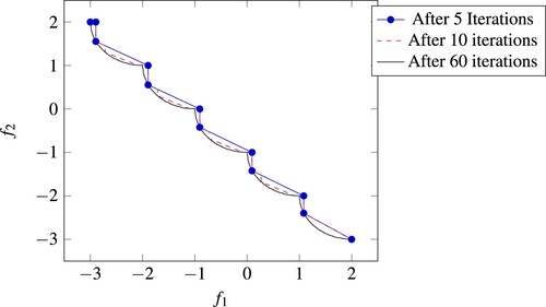
As a convex-quadratic benchmark problem we consider the problem described in Appendix 3, which is also used as problem (T4) in [2]. We use a setting with 2 continuous variables and a varying number of integer variables. Figure 9 shows a plot of the approximations generated by our algorithm for this problem (T4) with one integer variable. The use of segment patches allows our algorithm to adapt well to the curvature of the Pareto frontier, requiring only a small number of iterations until a very good approximation is achieved.

Figure 9. Illustration of the approximations of the Pareto frontier generated by our algorithm for problem (T4). The approximation created after iteration 5 has a difference volume of 0.038, after 10 iterations the difference volume has already reached 0.018, while with 60 iterations, the difference volume is smaller than 0.001.

In Table 1, we provide a comparison of the number of iterations our algorithm needed to reach a difference volume of 0.001 to the number of nodes in the branching tree required by the algorithm in [2]. The results suggest that our algorithm achieves a faster convergence due to the use of segments for the approximation instead of single points.

Table 1. Comparison of the required number of steps on instance (T4) for our algorithm with the required number of branching nodes reported in [2, Table 1].

Number of integer variables	1	2	3
Number of iterations by our algorithm until ${\delta }_{\mathrm{vol}}\le {10}^{-3}$	36	95	70
Number of branching nodes generated by the algorithm in [2]	749	3683	19,127

Note that the used stopping criteria are not equivalent but correspond to roughly similar levels of approximation quality.

5.3. A nonlinear convex problem

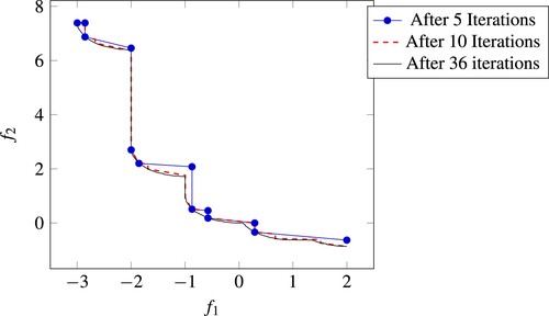
To illustrate the applicability of our algorithm on non-quadratic convex problems we use a problem which includes a non-polynomial term. This problem, featuring an exponential term, is also used as problem (T6) in [2] and given in detail in Appendix 4. Figure 10 shows a comparison of the approximations generated by our algorithm after different numbers of iterations.

Figure 10. Illustration of the approximations of the Pareto frontier generated by our algorithm for problem (T6). The approximation created after iteration 5 has a difference volume of 0.025, after 10 iterations the difference volume has already reached 0.009, and after 36 iterations, the difference volume is smaller than 0.001.

5.4. Computational results on linear mixed-integer problems

To complement the strong theoretical convergence rate we evaluate our algorithm on several mixed-integer linear programming benchmark problems. In order to obtain stable results, we apply the algorithm on many randomly generated instances of a problem type with same sizes. This allows to reduce deviations caused by single instances.

We use the following benchmark sets:

• The classic benchmark problem by Mavrotas and Diakoulaki [15] which is widely used in the literature. The exact specification of this synthetic problem is given in Appendix 5. We use the standard version of the problem, where the number of constraints, discrete and continuous variables are in a fixed proportion, thus requiring only a single size parameter.

• A capacitated facility location problem. We use it in a version with two objective functions containing all the variables but with independently generated coefficients. The size parameter describes the number of customers that is chosen equal to the number of possible facility locations. The detailed formulation is described in Appendix 6.

• The biobjective assignment benchmark used in [16] containing only integral variables, described in Appendix 7. Although our algorithm is not designed for this pure integer problem, the algorithm solves it with acceptable efficiency.

The Benchmark problems of Mavrotas and Diakoulaki

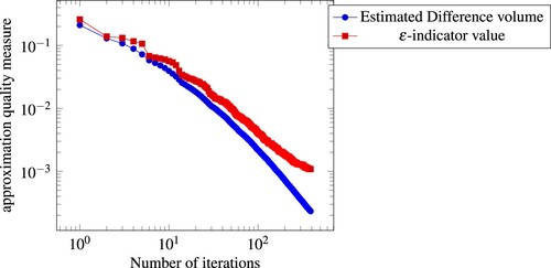
We illustrate the convergence of our algorithm by plotting the evolution of approximation quality measures against the number of iterations. We show both the difference volume which forms the basis of our algorithm, and the ε-indicator value as an alternative approximation quality measure for comparison purposes.

Such a log-log plot is shown in Figure 11 for the benchmark problem of Appendix 5 with 320 variables. The plots show the consistent convergence behaviour of the algorithm for all sizes of the underlying mixed-integer program, as long as the structure stays the same. The difference volume is decreasing consistently with the rate of a polynomial, after some initial iterations. In the log-log plot this is exhibited by an approximately straight line.

Figure 11. Dependence of the approximation quality on the number of iterations. Average over 10 instances of the benchmark problem by Mavrotas of Appendix 5 with 320 variables.

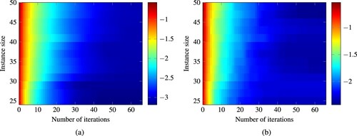
In Figure 12, the convergence of our algorithm on various instance sizes is illustrated. The figure shows that the number of needed iterations for similar accuracy values only increases slightly with larger instance sizes. The convergence of the difference volume is more consistent than the convergence of the ε-indicator value since the algorithm focuses on the difference volume.

Figure 12. Heatmap of the approximation quality reached after a given number of iterations for varying instance sizes of the benchmark of Mavrotas. The shade corresponds to the logarithm to the base 10 of the respective approximation quality measure. (a) Difference Volume, (b) e-indicator value.

Comparison to other algorithms

Since the benchmark problem by Mavrotas and Diakoulaki is widely used in the literature, it is well suited to perform a comparison of various algorithms. We compare our algorithm to results reported by the following papers that also use this benchmark problem:

• [17, Table 8.2],

• [19, Table 3],

• [4, Table 1], using the CT column,

• [3, Table 2 and Table 3], using results from the SIS-version of the algorithm (the version with the best performance on these instances),

• [39, Table 2], with accuracy parameter $\delta ={10}^{-2}$.

Although detailed running time results are provided, no clear guarantees of the approximation quality are given in the works above. Parameters that influence the resulting approximation quality are often specific to an algorithm and hard to compare. We report here the results corresponding to medium accuracy settings. However, the relative accuracy between the different algorithms is hard to estimate. For a better comparison, we also restrict the reviewed results to the simple form of the benchmark, with only binary and continuous variables. The used instance sizes are varying, however, all papers use the convention that the total number of variables always equals the number of constraints and exactly half of the variables are binary, respectively, continuous.

The comparison of the number of single-objective MIPs solved during the run of the algorithms in Figure 13 shows that this number increases in the case of our algorithm only slightly with larger instance sizes. Since our algorithm produces approximations iteratively with increasing approximation quality, we give the number of single-objective MIPs solved until a medium accuracy of a difference volume ${\delta }_{\mathrm{vol}}$ of ${10}^{-2}$, respectively, a high accuracy of a difference volume ${\delta }_{\mathrm{vol}}$ at most ${10}^{-3}$ is reached, as well as a very high accuracy of $2\cdot {10}^{-4}$ which is close to the numerical limits for the underlying MIP solver. The values for our algorithms are averages over 5 randomly generated instances each. Our number of MIPs to solve grows slower than that of other algorithms because of the faster convergence of our algorithm.

Figure 13. Comparison of the required number of MIP solutions by several algorithms for the benchmark problems by Mavrotas and Diakoulaki [15]. The instance size corresponds to the total number of variables.

In Figure 14, a comparison of the reported running times for various benchmark sizes is given. Note that the running times reported in the other papers were obtained with varying hardware and differing underlying solvers. Thus not all differences in the running times might be caused directly by the algorithms.

Figure 14. Comparison of running times required by several algorithms for the benchmark problems by Mavrotas and Diakoulaki [15]. The instance size corresponds to the total number of variables.

The comparison of Figure 14 shows that our algorithm is competitive with the algorithms in the literature. In particular, the asymptotic growth of the running time of our algorithm as a function of the instance size is significantly slower than for other algorithms. This allows our algorithm to compute good approximations for benchmark of double the size than previously considered in the literature (640 variables instead of previously 320) with a reasonable running time.

The results of [19, Table 13] provide running times measured until an approximation quality equivalent to a difference volume of 0.02 is reached. A comparison shows that our running time for a similar rough approximation (with a difference volume of ${10}^{-2}$) has an equivalent asymptotic growth rate.

The capacitated facility location benchmark

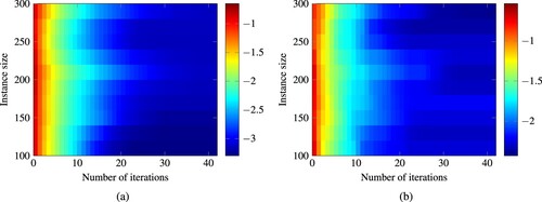
As a second benchmark problem we test our algorithm on the capacitated facility location problem. We consider here a bicriteria version where both continuous and discrete variables appear in both objectives, to create a characteristic bicriteria mixed-integer program, as detailed in Appendix 6. Figure 15 shows that our algorithm also exhibits a stable convergence for this benchmark. The number of needed iterations only increases slightly with larger instance sizes.

Figure 15. Heatmap of the approximation quality reached after a given number of iterations for varying instance sizes of the capacitated facility location benchmark. The shade corresponds to the logarithm to the base 10 of the respective approximation quality measure. (a) Difference Volume, (b) e-indicator value.

5.5. Behaviour on pure integer programs

Although our algorithm was designed for mixed-integer programs with a significant continuous component, it can also be used for multicriteria pure integer programs. The individual steps could be simplified in the case of a pure integer program, since a segment patch in this case always reduces to a single point. However, the following experiments show that the convergence behaviour is still competitive with other algorithms that are specialized on pure integer programs.

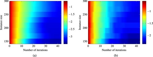
As a pure integer benchmark problem we use a biobjective assignment problem, which is described in detail in Appendix 7. Unlike problems with a significant continuous part, the Pareto frontier of instances of the biobjective assignment problem consists only of horizontal segments. Figure 16 shows that our algorithm nevertheless exhibits a satisfactory convergence on this problem.

Figure 16. Heatmap of the approximation quality after a given number of iterations for varying instance sizes of the biobjective assignment benchmark. The shade corresponds to the logarithm to the base 10 of the respective approximation quality measure. (a) Difference Volume, (b) e-indicator value.

Since the biobjective assignment benchmark was also used in [16], a numerical comparison is possible. In Figure 17, a comparison of the running times to our algorithm for various instance sizes is given. Although the algorithm in [16] is specialized for solving this type of pure integer biobjective problems, our algorithm is competitive with this algorithm.

Figure 17. Comparison of the running times of [16, Figure 11], using the best-performing variant BOBB-32, with running times for our algorithm. Note that for the instance size of 2025, the algorithm of [16] reaches its time limit of 300 s.

6. Conclusion and future work

In this paper, we presented the Adaptive Patch Approximation algorithm for approximating bicriteria convex mixed-integer programs based on patches. To our knowledge this is the first approximation algorithm for this class of problems that has a provable performance bound close to a non-trivial theoretical optimum, namely the segment patch complexity. This raises the question how this intrinsic property of a bicriteria mixed-integer program behaves. Which characteristics of a mixed-integer program are required in order to guarantee certain growth rates of the segment patch complexity? Our numerical results suggest that the segment patch complexity only grows slowly for practically relevant bicriteria MIPs ; however, a theoretical study of the underlying reasons iswarranted.

The numerical results show that the algorithm is competitive with other state-of-the-art methods. In order to make it even more usable in practice, several enhancements could be made:

• The algorithm could use the feedback provided by a user to dynamically focus on the part of the Pareto frontier that is currently most important to the decision making process.

• The transformed mixed-integer programs could be solved only approximately to obtain a speed-up. However, care has to be taken to ensure that the overall convergence properties of the algorithm are not affected.

• Instead of computing a segment patch given by just two points, patches with a higher number of base points could be used to better capture the curvature of the Pareto frontier.

Another goal is to extend this methodology to the case of optimization problems with three or more criteria. The notions of difference volume and patch complexity are also valid in this general case. However, several questions have to be answered to develop a generalization of the algorithm:

• What is a suitable higher-dimensional analogue of a segment patch?

• How can a convergence rate be shown that is within a small factor of the patch complexity?

• Which growth rate does the patch complexity have in higher dimensions?

Acknowledgments

The author is grateful to Ina Bertz and Karl-Heinz Küfer for providing valuable comments which improved the exposition. The author also would like to thank two anonymous reviewers and an associate editor for their detailed comments that lead to significant improvements of the clarity of the manuscript.

Disclosure statement

No potential conflict of interest was reported by the author.

Appendices

Appendix 1.

Proof of Proposition 3.2

In this section, we give a proof of Proposition 3.2 regarding the invariance of several measures under taking the monotone lower envelope.

Proof of Proposition 3.2.

Proof of Proposition 3.2.

Let $A=\bigcup _{i=1}^n{s}_i$ be an approximation consisting of a set of segments $s_1,\dots s_n$. Let $A^{\prime }$ denote the monotone lower envelope of $s_1,\dots s_n$.

We start with showing that the upper set is invariant under taking the nondominated set which excludes all dominated points, i.e. for a compact set $B\subseteq {\mathbb{R}}^2$ it holds $N\left(B\right)+{\mathbb{R}}_{\ge 0}^2=B+{\mathbb{R}}_{\ge 0}^2$. Note that the set A is compact as it is the finite union of bounded segments.

The inclusion $N\left(B\right)+{\mathbb{R}}_{\ge 0}^2\subseteq B+{\mathbb{R}}_{\ge 0}^2$ obviously holds since the nondominated set $N\left(B\right)\subseteq B$ is a subset of the original set. We thus only have to show the other inclusion. For this, let $(x,y)\in B+{\mathbb{R}}_{\ge 0}^2$ be a point in the upper set. Consider now a point $(x^{\prime },y^{\prime })\in \arg min\left\{a+b\mid (a,b)\in B,(x,y)\in (a,b)+{\mathbb{R}}_{\ge 0}^2\right\}$ which exists since $(x,y)\in B+{\mathbb{R}}_{\ge 0}^2$ guarantees that the set over which we minimize is nonempty and because $(a,b)\mapsto a+b$ is a continuous function over the compact set B. Then, it holds $(x^{\prime },y^{\prime })\in B$ and $(x^{\prime },y^{\prime })$ is not dominated by any other point in B, since this would contradict the minimality of $(x^{\prime },y^{\prime })$. Thus we have $(x^{\prime },y^{\prime })\in N\left(B\right)$ and therefore by construction $(x,y)\in N\left(B\right)+{\mathbb{R}}_{\ge 0}^2$.

1. We show that the corresponding nondominated sets $N\left(A\right)=N\left(A^{\prime }\right)$ coincide. Let $(x,y)\in N\left(A\right)$ be a nondominated point in the original set. Then, for all other points $(x^{\prime },y^{\prime })\in A$ it holds either $x^{\prime }>x$ or $y^{\prime }>y$. For all points in the monotone lower envelope $(a^{\prime },b^{\prime })\in A^{\prime }$ there exists by definition a point in the original set $(a,b)\in A$ such that $a^{\prime }\ge a$ and $b^{\prime }\ge b$ hold. Thus, we obtain in combination, that for all $(a^{\prime },b^{\prime })\in A^{\prime }$ it holds $a^{\prime }>x$ or $b^{\prime }>y$. Thus, $(x,y)\in N\left(A^{\prime }\right)$ is also a nondominated point in the monotone lower envelope. For the other direction, let $(x,y)\in N\left(A^{\prime }\right)$. Then, it must hold $(x,y)\in A$ since by construction of the monotone lower envelope for all points $(a,b)\in A^{\prime }\setminus A$ there exists a point $(a^{\prime },b)\in A$ with $a^{\prime }<a$, which would contradict the assumption that $(x,y)\in N\left(A^{\prime }\right)$ is nondominated. It only remains to show that $(x,y)$ is not dominated by any point in A. Suppose for the sake of contradiction that $(x,y)$ is dominated by a point in A. Then there exists a point $(x,y)\ne (x^{\prime },y^{\prime })\in A$ with $x^{\prime }\le x$ and $y^{\prime }\le y$. This implies that there also exists a point $(x^{″},y^{″})\in A^{\prime }$ with $x^{″}\le x^{\prime }$ and $y^{″}\le y^{\prime }$ by the definition of the monotone lower envelope. Thus, $(x^{″},y^{″})\in A^{\prime }$ would also dominate $(x,y)$, which contradicts the assumption that $(x,y)\in N\left(A^{\prime }\right)$ is nondominated. Thus, it must hold $(x,y)\in N\left(A\right)$.

2. We show now ${\delta }_{\mathrm{vol}}(Z,A)={\delta }_{\mathrm{vol}}(Z,A^{\prime })$. By using the previous property, it is sufficient to show that the ${\delta }_{\mathrm{vol}}(Z,A)$ only depends on the nondominated set of A. We use that $N\left(A{)}_y\right(x)=min\{y^{\prime }\mid (x,y^{\prime })\in N\left(A\right)+{\mathbb{R}}_{\ge 0}^2\}=min\{y^{\prime }\mid (x,y^{\prime })\in A+{\mathbb{R}}_{\ge 0}^2\}=A_y(x)$ is fulfilled since $N\left(A\right)+{\mathbb{R}}_{\ge 0}^2=A+{\mathbb{R}}_{\ge 0}^2$ holds by the properties of the nondominated set. Thus, using the representation (3(3) $\begin{array}{rl}{\delta }_{\mathrm{vol}}(Z,A)& =\mathrm{vol}\left(\left(\left(Z+{\mathbb{R}}_{\ge 0}^2\right)\setminus \left(A+{\mathbb{R}}_{\ge 0}^2\right)\right)\cap [0,1{]}^2\right)\\ & ={\int }_0^1{\int }_0^1{\mathbf{1}}_{\left(Z+{\mathbb{R}}_{\ge 0}^2\right)\setminus \left(A+{\mathbb{R}}_{\ge 0}^2\right)}(x,y)\mathrm{d}x\mathrm{d}y\\ & ={\int }_0^1\left({\int }_0^1{\mathbf{1}}_{\left(Z+{\mathbb{R}}_{\ge 0}^2\right)\setminus \left(A+{\mathbb{R}}_{\ge 0}^2\right)}(x,y)\mathrm{d}y\right)\mathrm{d}x\\ & ={\int }_0^1\left(A_y\right(x)-Z_y(x\left)\right)\mathrm{d}x.\end{array}$(3) ) for the difference volume, we obtain $\begin{array}{rl}{\delta }_{\mathrm{vol}}(Z,A)& ={\int }_0^1\left(A_y\right(x)-Z_y(x\left)\right)\mathrm{d}x={\int }_0^1\left(N\right(A{)}_y\left(x\right)-Z_y\left(x\right))\mathrm{d}x={\delta }_{\mathrm{vol}}(Z,N\left(A\right))\\ & ={\delta }_{\mathrm{vol}}(Z,N(A^{\prime }\left)\right)={\delta }_{\mathrm{vol}}(Z,A^{\prime }).\end{array}$

3. To show ${ϵ}_d\left(A\right)={ϵ}_d\left(A^{\prime }\right)$ we follow a similar strategy as for the previous point. We show that ${ϵ}_d\left(A\right)$ depends only on the nondominated set $N\left(A\right)$ which allows us then to apply the first statement. By using the fact $A+{\mathbb{R}}_{\ge 0}^2=N\left(A\right)+{\mathbb{R}}_{\ge 0}^2$, we obtain ${ϵ}_d(Z,A)=\underset{z\in Z+{\mathbb{R}}_{\ge 0}^2}{sup}\underset{x\in A+{\mathbb{R}}_{\ge 0}^2}{inf}||z-x|{|}_{\mathrm{\infty }}=\underset{z\in Z+{\mathbb{R}}_{\ge 0}^2}{sup}\underset{x\in N\left(A\right)+{\mathbb{R}}_{\ge 0}^2}{inf}||z-x|{|}_{\mathrm{\infty }}={ϵ}_d(Z,N(A\left)\right)$ proving that the value of ${ϵ}_d\left(A\right)$ is only dependent on the nondominated set, which implies with point (1) the equality ${ϵ}_d\left(A\right)={ϵ}_d\left(A^{\prime }\right)$.

Appendix 2.

Construction of linear inequalities to approximate the logarithm

In this appendix, we provide a proof for Lemma 4.1 by constructing a sequence of tangent points which yield a sufficient approximation of the logarithm.

Construction of the tangent points. We use tangents for the approximation at some positions $x_1,\dots ,x_k\in [0,1]$ which we need to find. The goal is to choose these positions such that the approximated value is always larger than $\ln \left(x\right)$, with an additive difference of at most ${\text{β}}^{\prime }$. Thus, at the position x = 1, the approximation should have a value of at most $\ln \left(1\right)+{\text{β}}^{\prime }={\text{β}}^{\prime }$. To minimize the number of line segments needed for the approximation, we should choose the value as large as allowed, i.e. the approximation at x = 1 should be exactly equal to ${\text{β}}^{\prime }$.

Let $x_0\in [0,1]$ be the touching point of the tangent. Since the tangent should have a value of ${\text{β}}^{\prime }$ at x = 1, we obtain the equality $\ln \left(x_0\right)+\frac{1-x_0}{x_0}={\text{β}}^{\prime },$ where we used $\frac{d}{dx}\ln \left(x\right)=\frac{1}{x}$. This equality leads to, using the condition $x_0\in [0,1]$, ${\text{β}}^{\prime }\ge 0$: $\begin{array}{rl}\ln \left(x_0\right)+\frac{1}{x_0}& ={\text{β}}^{\prime }+1\\ ⟺-\frac{1}{x_0}\exp \left(-\frac{1}{x_0}\right)& =-\exp (-{\text{β}}^{\prime }-1)\\ ⟺-\frac{1}{x_0}& =W_{-1}(-\exp (-{\text{β}}^{\prime }-1\left)\right)\\ ⟺x_0& =-\frac{1}{W_{-1}(-\exp (-{\text{β}}^{\prime }-1\left)\right)},\end{array}$ where $W_{-1}$ is the non-principal branch of the Lambert W function, i.e. for $-1/e\le z\le 0$, the value $W_{-1}\left(z\right)$ is the unique solution $w\le -1$ of $w\exp \left(w\right)=z$. The survey [40] provides an overview on the Lambert W function and its various applications.

We now search for the next position $z_1$ where an additive error of ${\text{β}}^{\prime }$ of the tangent through $x_0$ to the function $\ln \left(x\right)$ occurs. This position $z_1$ is characterized by the equation $\ln \left(x_0\right)+(z_1-x_0)\cdot \frac{1}{x_0}-\ln \left(z_1\right)={\text{β}}^{\prime },$ which can be equivalently transformed, using the substitution $z^{\prime }=\frac{z_1}{x_0}$, to $\begin{array}{rl}& z^{\prime }-\ln \left(x_0{z}^{\prime }\right)={\text{β}}^{\prime }+1-\ln \left(x_0\right)\\ & ⟺z^{\prime }-\ln \left(z^{\prime }\right)={\text{β}}^{\prime }+1\\ & ⟺z^{\prime }=-W(-\exp (-{\text{β}}^{\prime }-1\left)\right)\\ & ⟹z_1=x_0{z}^{\prime }=\frac{W_0(-\exp (-{\text{β}}^{\prime }-1\left)\right)}{W_{-1}(-\exp (-{\text{β}}^{\prime }-1\left)\right)},\end{array}$ where we used the principal branch $W_0$ of the Lambert W function to obtain a solution $z^{\prime }<1$. Otherwise, we would have obtained the solution $z^{\prime }=1$ which is obvious from the construction of $x_0$. The principal branch $W_0\left(z\right)$ is defined for values $z\ge -1$ as the unique solution $w\ge -1$ of $w\exp \left(w\right)=z$.

Recursive application. We now show that values for the other breakpoints scale in the same way.

Consider $x_1$, the touching position of the tangent such that the difference to the natural logarithm at position $z_1$ is ${\text{β}}^{\prime }$, which is characterized by the equation $\ln \left(x_1\right)+(z_1-x_1)\cdot \frac{1}{x_1}-\ln \left(z_1\right)={\text{β}}^{\prime }.$ Using the substitution $x_1^{\prime }=\frac{x_1}{z_1}$, we obtain the equivalent equation $\ln \left(x_1^{\prime }\right)+\frac{1}{x_1^{\prime }}={\text{β}}^{\prime }+1$ which has the exact same form as the equation for $x_0$, implying $x_1^{\prime }=x_1$ and by resubstitution $x_1=x_1^{\prime }\cdot z_1=x_0{z}_1$. We apply the analogous analysis for the position $z_2$ at which the difference of the tangent touching at $x_1$ has a difference of ${\text{β}}^{\prime }$ to the function ln. This leads to the equation $\ln \left(x_1\right)+(z_2-x_1)\cdot \frac{1}{x_1}-\ln \left(z_2\right)={\text{β}}^{\prime },$ which can be transformed via the substitution $z_2^{\prime }=\frac{z_2}{z_1}$ and using the result $x_1=z_1\cdot x_0$ to $\ln \left(x_0\right)+(z_2^{\prime }-x_0)\cdot \frac{1}{x_0}-\ln \left(z_2^{\prime }\right)={\text{β}}^{\prime }.$ Since this matches again the defining equation for $z_1$, we have $z_2^{\prime }=z_1$ and by resubstitution $z_2=z_2^{\prime }\cdot z_1=z_1^2$. For the next positions $z_3,z_4,\dots$ it follows analogously that $z_k=z_1^k$ for all $k\in \mathbb{N}$.

In order to obtain an additive approximation with an error at most ${\text{β}}^{\prime }$ on the interval $[{\delta }_0,1]$, we only need to choose the k tangents at the points $x_0,\dots x_{k-1}$ with the number of points k chosen such that $z_1^k\le {\delta }_0$ since this implies that only for values less than ${\delta }_0$ an additive error bigger than ${\text{β}}^{\prime }$ can occur. Solving this for k leads to $k=\lceil {\log }_{z_1}\left({\delta }_0\right)\rceil =⌈\frac{\ln \left({\delta }_0\right)}{\ln \left(z_1\right)}⌉=⌈\frac{\ln \left(1/{\delta }_0\right)}{\ln \left(1/z_1\right)}⌉,$ where $\lceil \cdot \rceil$ is the ceiling function. This shows that the dependence with respect to ${\delta }_0$ is logarithmic which implies that even for values of ${\delta }_0$ very close to 0 we only need a relative small number of tangents.

Bounding the step length. We now bound the value of $z_1$ from above in terms of ${\text{β}}^{\prime }$. This allows us to bound the number of tangents required to reach a certain approximation bound. For this we use the defining equation $z_1=\frac{W_0(-\exp (-{\text{β}}^{\prime }-1\left)\right)}{W_{-1}(-\exp (-{\text{β}}^{\prime }-1\left)\right)}.$ Since for all values ${\text{β}}^{\prime }\ge 0$ the values $W_0(-\exp (-{\text{β}}^{\prime }-1\left)\right)<0$ and $W_{-1}(-\exp (-{\text{β}}^{\prime }-1\left)\right)<0$ are negative, we need a lower bound for $W_0$ and an upper bound for $W_{-1}$. We use the following upper bound on $W_{-1}$ for all ${\text{β}}^{\prime }\ge 0$ shown in [41] $W_{-1}(-\exp (-{\text{β}}^{\prime }-1\left)\right)\le -1-\sqrt{2{\text{β}}^{\prime }}-\frac{2}{3}{\text{β}}^{\prime }\le -1-\sqrt{2{\text{β}}^{\prime }}.$ By inserting the trivial bound $W_0\left(x\right)\ge -1$ for all $x\ge -1/e$, we obtain $z_1=\frac{W_0(-\exp (-{\text{β}}^{\prime }-1\left)\right)}{W_{-1}(-\exp (-{\text{β}}^{\prime }-1\left)\right)}\le \frac{-1}{-1-\sqrt{2{\text{β}}^{\prime }}}=\frac{1}{1+\sqrt{2{\text{β}}^{\prime }}}.$ Finally, this yields the desired bound on the number of needed tangents: $k=⌈\frac{\ln \left(1/{\delta }_0\right)}{\ln \left(1/z_1\right)}⌉\le ⌈\frac{\ln \left(1/{\delta }_0\right)}{\ln (1+\sqrt{2{\text{β}}^{\prime }})}⌉,$ as ${\delta }_0>0$, exhibiting the asymptotic dependence of the number of needed linear inequalities for an additive accuracy ${\text{β}}^{\prime }$ close to 0.

Appendix 3.

Convex-quadratic benchmark problem

The benchmark problem is given as problem (T4) in [2]. We use it with two continuous variables and a configurable number m of integer variables. The problem has the form: (T4) $\begin{array}{rl}& min\left(x_1+\sum _{i=3}^{m+2}{x}_i,x_2-\sum _{i=3}^{m+2}{x}_i\right)\\ & \begin{array}{ll}\mathrm{s}.\mathrm{t}.& x_1^2+x_2^2\le 1\\ & x_i\in [-2,2]\mathrm{f}\mathrm{o}\mathrm{r}\mathrm{a}\mathrm{l}\mathrm{l}i=1,\dots ,m+2\\ & x_1,x_2\in \mathbb{R}\\ & x_i\in \mathbb{Z}\mathrm{f}\mathrm{o}\mathrm{r}\mathrm{a}\mathrm{l}\mathrm{l}i=3,\dots ,m+2\end{array}\end{array}$(T4)

Appendix 4.

Nonlinear convex benchmark problem

This nonlinear but convex mixed-integer problem is also given as problem (T6) in [2]. (T6) $\begin{array}{rl}& min\left(x_1+x_3,x_2+\exp (-x_3)\right)\\ & \begin{array}{ll}\mathrm{s}.\mathrm{t}.& x_1^2+x_2^2\le 1\\ & x_i\in [-2,2]\mathrm{f}\mathrm{o}\mathrm{r}\mathrm{a}\mathrm{l}\mathrm{l}i=1,\dots ,3\\ & x_1,x_2\in \mathbb{R}\\ & x_3\in \mathbb{Z}\end{array}\end{array}$(T6)

Appendix 5.

Benchmark problem of Mavrotas and Diakoulaki

The benchmark multicriteria MIP proposed in [15] is widely used in the literature for numerical studies. It is a randomly generated synthetic problem. We follow here roughly the presentation in [39] and restrict it to the case of two criteria to simplify notation. Additionally, we change the optimization direction to minimization. The problem has the following form, where x and y are the decision variables: $\begin{array}{rl}& min\left(\sum _{i=1}^n{c}_i^{\left(1\right)}{x}_i+\sum _{j=1}^q{f}_j^{\left(1\right)}{y}_j,\sum _{i=1}^n{c}_i^{\left(2\right)}{x}_i+\sum _{j=1}^q{f}_j^{\left(2\right)}{y}_j\right)\\ & \begin{array}{ll}\mathrm{s}.\mathrm{t}.& \sum _{i=1}^n{a}_{ij}{x}_i+a_j^{\prime }{y}_j\le b_j\mathrm{f}\mathrm{o}\mathrm{r}\mathrm{a}\mathrm{l}\mathrm{l}j=1\dots ,q\\ & \sum _{i=1}^n{a}_{ij}{x}_i\le b_j\mathrm{f}\mathrm{o}\mathrm{r}\mathrm{a}\mathrm{l}\mathrm{l}j=q+1,\dots ,m-1\\ & \sum _{j=1}^q{y}_j\le \frac{q}{3}\\ & x_i\in {\mathbb{R}}_{\ge 0}\mathrm{f}\mathrm{o}\mathrm{r}\mathrm{a}\mathrm{l}\mathrm{l}i=1,\dots ,n\\ & y_j\in \{0,1\}\mathrm{f}\mathrm{o}\mathrm{r}\mathrm{a}\mathrm{l}\mathrm{l}j=1,\dots ,q\end{array}\end{array}$

The parameter m denotes the total number of constraints, the number of continuous variables is denoted by n and the number of binary variables is given by q. We randomly generate the coefficients independently according to the following uniform distributions:

• $c_i^{\left(1\right)},c_i^{\left(2\right)}\sim \mathcal{U}\left(\right[-10,10\left]\right)$, $i=1,\dots ,n$

• $f_j^{\left(1\right)},f_j^{\left(2\right)}\sim \mathcal{U}\left(\right[-200,200\left]\right)$, $j=1,\dots ,q$

• $b_j\sim \mathcal{U}\left(\right[50,100\left]\right)$, $j=1,\dots ,m-1$

• $a_{ij},a_j^{\prime }\sim \mathcal{U}\left(\right[-1,20\left]\right)\circ B\left(0.25\right)$

where $\mathcal{U}\left(\right[-1,20\left]\right)\circ B\left(0.25\right)$ denotes the distribution with values having a value of 0 with a probability of 0.75 and otherwise uniform values in $[-1,20]$.

Appendix 6.

Capacitated facility location problem

The capacitated facility location problem consists of a set I of $n=|I|$ many possible facility locations that should serve a set J of customers (here chosen to also have cardinality $|J|=n$). A corresponding cost occurs for each opened facility as well as each unit transported from a facility to a customer. We use two independent sets of cost coefficients for the two objective functions, each including all decision variables. The bicriteria capacitated facility location problem is formally given as: $\begin{array}{rl}& min\left(\sum _{i\in I}\sum _{j\in J}{c}_{ij}^{\left(1\right)}{y}_{ij}+\sum _{i=1}^n{f}_i^{\left(1\right)}{x}_i,\sum _{i\in I}\sum _{j\in J}{c}_{ij}^{\left(2\right)}{y}_{ij}+\sum _{i=1}^n{f}_i^{\left(2\right)}{x}_i\right)\\ & \begin{array}{ll}\mathrm{s}.\mathrm{t}.& \sum _{i=1}^n{y}_{ij}=1\mathrm{f}\mathrm{o}\mathrm{r}\mathrm{a}\mathrm{l}\mathrm{l}j\in J\\ & \sum _{j\in J}{y}_{ij}\le u_i{x}_i\mathrm{f}\mathrm{o}\mathrm{r}\mathrm{a}\mathrm{l}\mathrm{l}i\in I\\ & y_{ij}\in {\mathbb{R}}_{\ge 0}\mathrm{f}\mathrm{o}\mathrm{r}\mathrm{a}\mathrm{l}\mathrm{l}i\in I,j\in I\\ & x_i\in \{0,1\}\mathrm{f}\mathrm{o}\mathrm{r}\mathrm{a}\mathrm{l}\mathrm{l}i\in I\end{array}\end{array}$ Here, the coefficients $c_{ij}^{\left(1\right)}$, $c_{ij}^{\left(2\right)}$ represent the transportation cost per unit, $f_i^{\left(1\right)}$, $f_i^{\left(2\right)}$ the cost for opening a facility and $u_i$ the maximal capacity of a facility. The variable $x_i$ indicates whether facility $i\in I$ is opened and $y_{ij}$ describes the amount sent from facility i to customer j. We generate the coefficients randomly as follows, all independently from each other:

• We sample the transportation cost coefficients $c_{ij}^{\left(1\right)}$ and $c_{ij}^{\left(2\right)}$, $i\in I$, $j\in J$ uniformly from the interval $[1,2]$.

• We sample the facility opening costs $f_i^{\left(1\right)}$ and $f_i^{\left(2\right)}$, $i\in I$ uniformly from the interval $[0,10]$.

• The capacity values $u_i$, $i\in I$ are sampled uniformly from the interval $[1,10]$.

Appendix 7.

Biobjective assignment problem

The biobjective assignment problem asks to find an assignment between two sets. There are weights for each possible chosen assignment. The goal is to minimize this total weight. For each of the objectives, the weights are different. We use the random generation as described in [16, Appendix 1]. Formally, the problem can be given as: $\begin{array}{rl}& min\left(\sum _{i=1}^n\sum _{j=1}^n{c}_{ij}^{\left(1\right)}{x}_{ij},\sum _{i=1}^n\sum _{j=1}^n{c}_{ij}^{\left(2\right)}{x}_{ij}\right)\\ & \begin{array}{ll}\mathrm{s}.\mathrm{t}.& \sum _{i=1}^n{x}_{ij}=1\mathrm{f}\mathrm{o}\mathrm{r}\mathrm{a}\mathrm{l}\mathrm{l}j=1,\dots ,n\\ & \sum _{j=1}^n{x}_{ij}=1\mathrm{f}\mathrm{o}\mathrm{r}\mathrm{a}\mathrm{l}\mathrm{l}i=1,\dots ,n\\ & x_{ij}\in \{0,1\}\mathrm{f}\mathrm{o}\mathrm{r}\mathrm{a}\mathrm{l}\mathrm{l}i,j=1,\dots ,n\end{array}\end{array}$ We choose the objective function coefficients $c_{ij}^{\left(1\right)}$ and $c_{ij}^{\left(2\right)}$ randomly independently from the uniform distribution $\mathcal{U}\left(\right[0,20\left]\right)$.

References

- Ruzika S, Wiecek MM. Approximation methods in multiobjective programming. J Optim Theor Appl. 2005;126(3):473–501.
- de Santis M, Eichfelder G, Niebling J, et al. Solving multiobjective mixed integer convex optimization problems. SIAM J Optim. 2020;30(4):3122–3145.
- Perini T, Boland N, Pecin D, et al. A criterion space method for biobjective mixed integer programming: the boxed line method. Inf J Comput. 2020;32(1):16–39.
- Fattahi A, Turkay M. A one direction search method to find the exact nondominated frontier of biobjective mixed-binary linear programming problems. Eur J Oper Res. 2018;266(2):415–425.
- Laumanns M, Thiele L, Zitzler E. An efficient, adaptive parameter variation scheme for metaheuristics based on the epsilon-constraint method. Eur J Oper Res. 2006;169(3):932–942.
- Dächert K, Klamroth K. A linear bound on the number of scalarizations needed to solve discrete tricriteria optimization problems. J Global Optim. 2015;61(4):643–676.
- Rote G. The convergence rate of the sandwich algorithm for approximating convex functions. Computing. 1992;48(3-4):337–361.
- Gruber PM, Kenderov P. Approximation of convex bodies by polytopes. Rend Circ Mat Palermo. 1982;31(2):195–225.
- Zitzler E, Thiele L. Multiobjective evolutionary algorithms: a comparative case study and the strength pareto approach. IEEE Trans Evol Comput. 1999;3(4):257–271.
- Faulkenberg SL, Wiecek MM. On the quality of discrete representations in multiple objective programming. Optim Eng. 2010;11(3):423–440.
- Vassilvitskii S, Yannakakis M. Efficiently computing succinct trade-off curves. Theor Comput Sci. 2005;348(2-3):334–356.
- Kim IY, de Weck OL. Adaptive weighted sum method for multiobjective optimization: a new method for Pareto front generation. Struct Multidiscip Optim. 2006;31(2):105–116.
- Eichfelder G. Scalarizations for adaptively solving multi-objective optimization problems. Comput Optim Appl. 2009;44(2):249–273.
- Cacchiani V, D'Ambrosio C. A branch-and-bound based heuristic algorithm for convex multi-objective MINLPs. Eur J Oper Res. 2017;260(3):920–933.
- Mavrotas G, Diakoulaki D. A branch and bound algorithm for mixed zero-one multiple objective linear programming. Eur J Oper Res. 1998;107(3):530–541.
- Stidsen T, Andersen KA, Dammann B. A branch and bound algorithm for a class of biobjective mixed integer programs. Manage Sci. 2014;60(4):1009–1032.
- Belotti P, Soylu B, Wiecek MM. Fathoming rules for biobjective mixed integer linear programs: review and extensions. Discrete Optim. 2016;22:341–363.
- Cabrera-Guerrero G, Ehrgott M, Mason AJ, et al. Bi-objective optimisation over a set of convex sub-problems. Ann Oper Res. 2021. https://doi.org/10.1007/s10479-020-03910-3.
- Boland N, Charkhgard H, Savelsbergh M. A criterion space search algorithm for biobjective mixed integer programming: the triangle splitting method. Inf J Comput. 2015;27(4):597–618.
- Reuter H. An approximation method for the efficiency set of multiobjective programming problems. Optimization. 1990;21(6):905–911.
- Serna Hernández JI. Multi-objective optimization in mixed integer problems: with application to the beam selection optimization problem in IMRT [Ph.D thesis]. Berlin: mbv, Mensch-und-Buch-Verlag, TU Kaiserslautern; 2011.
- Teichert K, Süss P, Serna JI, et al. Comparative analysis of Pareto surfaces in multi-criteria IMRT planning. Phys Med Biol. 2011;56(12):3669–3684.
- Mavrotas G, Diakoulaki D. Multi-criteria branch and bound: a vector maximization algorithm for mixed 0-1 multiple objective linear programming. Appl Math Comput. 2005;171(1):53–71.
- Vincent T, Seipp F, Ruzika S, et al. Multiple objective branch and bound for mixed 0-1 linear programming: corrections and improvements for the biobjective case. Comput Oper Res. 2013;40(1):498–509.
- Zilberstein S, Russell S. Approximate reasoning using anytime algorithms. In: Natarajan S, editor. Imprecise and approximate computation. Boston: Kluwer; 1995. p. 43–62.
- Ehrgott M. Multicriteria optimization. Berlin, Heidelberg: Springer; 2005.
- Laszczyk M, Myszkowski PB. Survey of quality measures for multi-objective optimization: construction of complementary set of multi-objective quality measures. Swarm Evol Comput. 2019;48:109–133.
- Auger A, Bader J, Brockhoff D, et al. Hypervolume-based multiobjective optimization: theoretical foundations and practical implications. Theor Comput Sci. 2012;425:75–103.
- Wu J, Azarm S. Metrics for quality assessment of a multiobjective design optimization solution set. J Mech Des. 2001;123(1):18–25.
- Zitzler E, Thiele L, Laumanns M, et al. Performance assessment of multiobjective optimizers: an analysis and review. IEEE Trans Evol Comput. 2003;7(2):117–132.
- Loridan P. Epsilon-solutions in vector minimization problems. J Optim Theor Appl. 1984;43(2):265–276.
- Legriel J, Le Guernic C, Cotton S, et al. Approximating the Pareto front of multi-criteria optimization problems. In: Hutchison D, Kanade T, Kittler J, et al., editors. Tools and algorithms for the construction and analysis of systems. Berlin, Heidelberg: Springer; 2010. p. 69–83.
- Diessel E. Efficiently computing the approximation quality of Pareto frontiers. Optimization. 2020; http://www.optimization-online.org/DB_HTML/2020/09/8036.html.
- Bazgan C, Jamain F, Vanderpooten D. Approximate Pareto sets of minimal size for multi-objective optimization problems. Oper Res Lett. 2015;43(1):1–6.
- Tagansky B. A new technique for analyzing substructures in arrangements of piecewise linear surfaces. Discrete Comput Geom. 1996;16(4):455–479.
- Hart S, Sharir M. Nonlinearity of Davenport-Schinzel sequences and of generalized path compression schemes. Combinatorica. 1986;6(2):151–177.
- Hsiung KL, Kim SJ, Boyd S. Tractable approximate robust geometric programming. Optim Eng. 2008;9(2):95–118.
- Gurobi Optimization, LLC. Gurobi optimizer reference manual; 2020. http://www.gurobi.com.
- Rasmi SAB, Türkay M. GoNDEF: an exact method to generate all non-dominated points of multi-objective mixed-integer linear programs. Optim Eng. 2019;20(1):89–117.
- Corless RM, Gonnet GH, Hare DEG, et al. On the Lambert W function. Adv Comput Math. 1996;5(1):329–359.
- Chatzigeorgiou I. Bounds on the Lambert function and their application to the outage analysis of user cooperation. IEEE Commun Lett. 2013;17(8):1505–1508.