
 ?Mathematical formulae have been encoded as MathML and are displayed in this HTML version using MathJax in order to improve their display. Uncheck the box to turn MathJax off. This feature requires Javascript. Click on a formula to zoom.
Abstract
We present a reformulation of optimization problems over the Stiefel manifold by using a Cayley-type transform, named the generalized left-localized Cayley transform, for the Stiefel manifold. The reformulated optimization problem is defined over a vector space, whereby we can apply directly powerful computational arts designed for optimization over a vector space. The proposed Cayley-type transform enjoys several key properties which are useful to (i) study relations between the original problem and the proposed problem; (ii) check the conditions to guarantee the global convergence of optimization algorithms. Numerical experiments demonstrate that the proposed algorithm outperforms the standard algorithms designed with a retraction on the Stiefel manifold.
1. Introduction
The Stiefel manifold is defined for
with
, where
is the
identity matrix (see Appendix 1 for basic facts on
).
We consider an orthogonal constraint optimization problem formulated as:
Problem 1.1
For a given continuous function ,
(1)
(1) where the existence of a minimizer in (Equation1
(1)
(1) ) is automatically guaranteed by the compactness of
and the continuity of f over the Np-dimensional Euclidean space
.
This problem belongs to the so-called Riemannian optimization problems (see [Citation1] and Appendix 2), and has rich applications, in the case in particular, in data sciences including signal processing and machine learning as remarked recently in [Citation2,Citation3]. These applications include, e.g. nearest low-rank correlation matrix problem [Citation4–6], nonlinear eigenvalue problem [Citation7–9], sparse principal component analysis [Citation10–12], 1-bit compressed sensing [Citation13,Citation14], joint diagonalization problem for independent component analysis [Citation15–17] and enhancement of the generalization performance in deep neural network [Citation18,Citation19]. However, Problem 1.1 has inherent difficulties regarding the severe nonlinearity of
as an instance of general nonlinear Riemannian manifolds.
Minimization of a continuous over the orthogonal group
is a special instance of Problem 1.1 with p = N. This problem can be separated into two optimization problems over the special orthogonal group
as
(2)
(2) and, with an arbitrarily chosen
,
because
is the disjoint union of
and
. For the problem in (Equation2
(2)
(2) ), the Cayley transform
(3)
(3) and its inversion mappingFootnote1
(4)
(4) have been utilized in [Citation18,Citation20,Citation21] because φ translates a subset
[see (A3)]) of
into the vector space
of all skew-symmetric matrices, where
is called, in this paper, the singular-point set of φ. More precisely, this is because φ is a diffeomorphism between the dense subsetFootnote2
of
and
.
The Cayley transform pair φ and can be modified with an arbitrarily chosen
as
(5)
(5) and
(6)
(6) where
is the singular-point set of
. These mappings are also diffeomorphisms between their domains and images. With the aid of
Footnote3 with
, the following Problem 1.2 was considered in [Citation20] as a relaxation of the problem in (Equation2
(2)
(2) ).
Problem 1.2
For a given continuous function , choose
, and
arbitrarily. Then,
(7)
(7)
Remark 1.3
(The existence of
in Problem 1.2). The existence of
(Left-localized Cayley transform). We call
We note that Problem 1.2 is a realistic relaxation of the problem in (Equation2(2)
(2) ) as long as our target is approximation of a solution to (Equation2
(2)
(2) ) algorithmically because
is dense in
. In reality with a digital computer, we can handle just a small subset of the rational numbers
, which is dense in
, due to the limitation of the numerical precision. This situation implies that it is reasonable to consider an approximation of
within its dense subset
.
For Problem 1.2, we can enjoy various arts of optimization over a vector space, e.g. the gradient descent method and Newton's method, because is a vector space. Thanks to the homeomorphism of
, we can estimate a solution to the problem in (Equation2
(2)
(2) ) by applying
to a solution of Problem 1.2 with a sufficiently small
. We call this strategy via Problem 1.2 a Cayley parametrization (CP) strategy for the problem in (Equation2
(2)
(2) ). The CP strategy has a notable advantage over the standard optimization strategies [Citation1], called the retraction-based strategies, in view that many powerful computational arts designed for optimization over a single vector space can be directly plugged into the CP strategy. We will discuss the details in Remark 3.6.
In this paper, we address a natural question regarding a possible extension of the CP strategy to Problem 1.1 for general p<N: can we parameterize a dense subset of even with p<N in terms of a single vector space? To answer this question positively, we propose a Generalized Left-Localized Cayley Transform (G-L
CT):
with
, as an extension of the left-localized Cayley transform
in (Equation5
(5)
(5) ), where
and
are determined with a centre point
(see (Equation11
(11)
(11) ) and (Equation12
(12)
(12) ) in Definition 2.1). The set
is called the singular-point set of
(see the notation in the end of this section), and
is a linear subspace of
(see (Equation9
(9)
(9) )). For any
, we will show several key properties, e.g. (i)
is a diffeomorphism between
and the vector space
with the inversion mapping
(see Proposition 2.2); (ii)
is a dense subset of
for p<N (see Theorem 2.3(b)). Therefore, the proposed
and
have inherent properties desired for applications in the CP strategy to Problem 1.1.
To extend the CP strategy to Problem 1.1 for p<N, we consider Problem 1.4 below, which can be seen as an extension of Problem 1.2. For the same reason as in Remark 1.3(a), the existence of achieving (Equation8
(8)
(8) ) is guaranteed by the denseness of
in
(see Lemma 2.6).
Problem 1.4
For a given continuous function with p<N, choose
, and
arbitrarily. Then,
(8)
(8)
Under a smoothness assumption on general f, a realistic goal for Problem 1.1 is to find a stationary point of f because Problem 1.1 is a non-convex optimization problem (see, e.g. [Citation1,Citation22,Citation23]) and any local minimizer must be a stationary point [Citation22,Citation23]. In Lemma 3.4, we present a characterization of a stationary point
of f over
, with
satisfying
, in terms of a stationary point
of
over the vector space
, i.e.
. To approximate a stationary point of f over
, we also consider the following problem:
Problem 1.5
For a continuously differentiable function with p<N, choose
and
arbitrarily. Then,
For Problem 1.5, we can apply many powerful arts for searching a stationary point of a non-convex function over a vector space.
Numerical experiments in Section 4 demonstrate that the proposed CP strategy outperforms the standard algorithms designed with a retraction on (see Appendix 2) in the scenario of a certain eigenbasis extraction problem.
Notation. and
denote the set of all positive integers and the set of all real numbers respectively. For general
, we use
for the identity matrix in
, but for simplicity, we use
for the identity matrix in
. For
,
denotes the matrix of the first p columns of
. For a matrix
,
denotes the
entry of
, and
denotes the transpose of
. For a square matrix
we use the notation
for
. For
, the matrices
and
respectively denote the upper and the lower block matrices of
. For
, the matrices
and
respectively denote the left and right block matrices of
. For a matrix
,
denotes the skew-symmetric component of
. For square matrices
,
denotes the block diagonal matrix with diagonal blocks
. For a given matrix,
and
denote the spectral norm and the Frobenius norm respectively. The functions
and
denote respectively the largest and the nonnegative smallest singular values of a given matrix. The function
denotes the largest eigenvalue of a given symmetric matrix. For a vector space
of matrices,
denotes an open ball centred at
with radius
. To distinguish from the symbol for the orthogonal group
, the symbol
is used in place of the standard big O notation for computational complexity.
2. Generalized left-localized Cayley transform (G-LCT)
2.1. Definition and properties of G-LCT
In this subsection, we introduce the Generalized Left-Localized Cayley Transform (G-LCT) for the parametrization of
as a natural extension of
in (Equation5
(5)
(5) ). Indeed, the G-L
CT inherits key properties satisfied by
(see Proposition 2.2 and Theorem 2.3).
Definition 2.1
Generalized left-localized Cayley transform
For satisfying
, let
,
, and
(9)
(9) The generalized left-localized Cayley transform centred at
is defined by
(10)
(10) with
(11)
(11)
(12)
(12) where we call
the centre point of
, and
the singular-point set of
.
Proposition 2.2
Inversion of G-LCT
The mapping with
is a diffeomorphism between a subset
and
.Footnote4 The inversion mapping is given, in terms of
in (Equation6
(6)
(6) ), by
(13)
(13) where
. Moreover, for
, we have the following expressions
(14)
(14)
(15)
(15) where
is the Schur complement matrix of
(see Fact A.6).
Proof.
See Appendix 3.
Theorem 2.3
Denseness of
Let and p<N. Then, the following hold:
For
Let
Proof.
See Appendix 4.
Proposition 2.4
Properties of G-LCT in view of the manifold theory
(Chart). For
(Smooth atlas). The set
Proof.
(a) (i) See Theorem 2.3(b). (ii) From Proposition 2.2, is a homeomorphism between
and
. Clearly the dimension of the vector space
is
.
(b) (i) Recall that . (ii) See Proposition 2.2.
Remark 2.5
(Relation between the Cayley transform-based retraction and
(Parametrization of
(On the choice of
By using Theorem 2.3, we deduce Lemma 2.6, which guarantees the existence of a solution to Problem 1.4 for any . Theorem 2.3 will also be used in Lemma 3.5 to ensure the existence of a solution to Problem 1.5.
Lemma 2.6
Let be continuous with p<N and
. Then, it holds
(16)
(16)
Proof.
The second equality in (Equation16(16)
(16) ) is verified from the homeomorphism of
. Let
be a global minimizer of f over
, i.e.
. From the denseness of
in
(see Theorem 2.3(b)), there exists a sequence
satisfying
. The continuity of f yields
, i.e.
.
2.2. Computational complexities for and with
From the expressions in (Equation10(10)
(10) )–(Equation12
(12)
(12) ) and (Equation15
(15)
(15) ), both
and
with general
require
flops (FLoating-point OPerationS [not ‘FLoating point Operations Per Second’]), which are dominated by the matrix multiplications
in (Equation12
(12)
(12) ) and
in (Equation15
(15)
(15) ) respectively. However, if we employ a special centre point
(17)
(17) then the complexities for
and
can be reduced to
flops. Indeed, for
and
, we have
and
. Hence
requires
flops due to
Moreover, for
and
, it follows from
and (Equation15
(15)
(15) ) that
requires
flops.
For a given , Theorem 2.7 below presents a way to select
satisfying
, where
is designed with a singular value decomposition of
, requiring thus at most
flops.
Theorem 2.7
Parametrization of by with
Let , and
be a singular value decomposition of
, where
and
is a diagonal matrix with non-negative entries. Define
with
. Then, the following hold:
Proof.
(a) By , it holds
, which implies
by Definition 2.1.
(b) Substituting and
into (Equation11
(11)
(11) ) and (Equation12
(12)
(12) ), we obtain (Equation18
(18)
(18) ). From (Equation12
(12)
(12) ),
is bounded above as
(19)
(19)
Remark 2.8
Comparisons to commonly used retractions of
The computational complexity flops for
with
is competitive to that for commonly used retractions, which map a tangent vector to a point in
(for the retraction-based strategy, see Appendix 2). Indeed, retractions based on QR decomposition, the polar decomposition [Citation1] and the Cayley transform [Citation22] require respectively
flops,
flops and
flops [Citation24, Table ].
Table 1. Performance of each algorithm applied to Problem 4.1.
2.3. Gradient of function after the Cayley parametrization
For the applications of (G-L
CT) with
to Problems 1.4 and 1.5, we present an expression of the gradient of
denoted by
(Proposition 2.9) and its useful properties (Proposition 2.10, Remark 2.11 and also Proposition A.11).
Proposition 2.9
Gradient of function after the Cayley parametrization
For a differentiable function and
, the function
is differentiable with
(20)
(20) where
(21)
(21) and
(22)
(22)
(23)
(23) in terms of
and
. In particular, by
in (Equation13
(13)
(13) ),
(24)
(24)
Proof.
See Appendix 6.
Proposition 2.10
Transformation formula for gradients of function
For , suppose that
and
satisfy
. Then, for a differentiable function
, the following hold:
Proof.
See Appendix 7.
Remark 2.11
(Computational complexity for
(Relation of gradients after Cayley parametrization). Proposition 2.10 illustrates the relations of two gradients after Cayley parameterization with different centre points. These relations will be used in Lemmas 3.4 and 3.5 to characterize the first-order optimality condition with the proposed Cayley parametrization.
(Useful properties of the gradient after Cayley parametrization). In Appendix 8, we present useful properties (i) Lipschitz continuity; (ii) the boundedness; (iii) the variance bounded; of
3. Optimization over the Stiefel manifold with the Cayley parametrization
3.1. Optimality condition via the Cayley parametrization
We present simple characterizations of (i) local minimizer, and (ii) stationary point, of a real valued function over in terms of
.
Let be a vector space of matrices. A point
is said to be a local minimizer of
over
if there exists
satisfying
for all
. Under the smoothness assumption on J,
is said to be a stationary point of J over the vector space
if
. For a smooth function
,
is said to be a stationary point of f over
[Citation22,Citation23] if
satisfies the following conditions:
(26)
(26) The above conditions
and (Equation26
(26)
(26) ) are called the first-order optimality conditions because they are respectively necessary conditions for
to be a local minimizer of J over
(see, e.g. [Citation33, Theorem 2.2]), and for
to be a local minimizer of f over
(see [Citation23, Definition 2.1, Remark 2.3] and [Citation22, Lemma 1]).
In Lemma 3.1 below, we characterize a local minimizer of f over as a local minimizer of
with a certain
over the vector space
.
Lemma 3.1
Equivalence of local minimizers in the two senses
Let be continuous. Let
and
satisfy
. Then,
is a local minimizer of f over
if and only if
is a local minimizer of
over the vector space
.
Proof.
Let be a local minimizer of f over
and
satisfy
for all
. From the homeomorphism of
in Proposition 2.2,
is a nonempty open subset of
containing
. Then, there exists
satisfying
. Since
, we obtain
for all
, implying thus
is a local minimizer of
over
. In a similar way, we can prove its converse.
Under a special assumption on f in Theorem 3.2 below, yet found especially in many data science scenarios (see Remark 3.3), we can characterize a global minimizer of Problem 1.1 via with any
. In this case, a global minimizer
of
is guaranteed to exist in the unit ball
.
Theorem 3.2
Let . Assume that
is continuous and right orthogonal invariant, i.e.
for
and
. Then, there exists a global minimizer
of
achieving
,
and
.
Proof.
Let be a global minimizer of f over
, and
be a singular value decomposition with
and nonnegative-valued diagonal matrix
. Then, we obtain
with
by
. The right orthogonal invariance of f ensures
with
.
Substituting into (Equation11
(11)
(11) ) and (Equation12
(12)
(12) ), we obtain
and
. In a similar manner to (Equation19
(19)
(19) ), the last equality implies
. The last statement is verified by
Remark 3.3
Right orthogonal invariance
Under the right orthogonal invariance of f, Problem 1.1 arises in, e.g. low-rank matrix completion [Citation34,Citation35], eigenvalue problems [Citation1,Citation22,Citation24,Citation36], and optimal model reduction [Citation3,Citation37]. These applications can be formulated as optimization problems over the Grassmann manifold
, which is the set of all p-dimensional subspace of
. Practically,
is represented numerically by
, where
is an equivalence class, because the column space of
equals that of
for all
. Since the value of the right orthogonal invariant f depends only on the equivalence class
, Problem 1.1 of such f can be regarded as an optimization problem over
.
In Lemma 3.4 below, we characterize a stationary point of f over by a stationary point of
with a certain
over the vector space
. Moreover, Lemma 3.5 ensures the existence of solutions to Problem 1.5 with any
. Therefore, we can approximate a stationary point of f over
by solving Problem 1.5 with a sufficiently small
.
Lemma 3.4
First-order optimality condition
Let be differentiable. Let
and
satisfy
. Then, the first-order optimality condition in (Equation26
(26)
(26) ) can be stated equivalently as
(27)
(27) where
.
Proof.
Let satisfy
. Then, we have
. For
satisfying
and
, i.e.
, Proposition 2.10(c) asserts that
if and only if
. To prove the equivalence between (Equation26
(26)
(26) ) and (Equation27
(27)
(27) ), it is sufficient to show the equivalence between the condition in (Equation26
(26)
(26) ) and
. By (Equation24
(24)
(24) ), we have
which yields
if and only if the second condition in (Equation26
(26)
(26) ) holds true.
In the following, we show the equivalence of and
. By noting
, the equality
implies
. Conversely,
implies
.
Lemma 3.5
Let be continuously differentiable with p<N and
. Then,
.
Proof.
Let be a global minimizer of f over
, and
satisfy
. Then,
is a stationary point of f over
, and we have
with
from Lemma 3.4.
Theorem 2.3(c) ensures the denseness of in
. Then, we obtain a sequence
of
converging to
. Let
and
be sequences of
and
. The continuity of
yields
, implying the boundedness of
. From
and Proposition 2.10(b), we have
. The right-hand side of the above inequality converges to zero from the boundedness of
and
. Therefore, we have
, from which we completed the proof.
3.2. Basic framework to incorporate optimization techniques designed over a vector space with the Cayley parametrization
We illustrate a general scheme of the Cayley parametrization strategy in Algorithm 1,Footnote5 where is an initial estimate for a solution to Problem 1.1 with p<N,
is a centre point for parametrization of a dense subset
in terms of the vector space
, and a mapping
is a certain update rule for decreasing the value of
. In principle, we can employ any optimization update scheme over a vector space as
, which is a notable advantage of the proposed strategy over the standard strategy (see Remark 3.6). As a simplest example, we will employ, in Section 4, a gradient descent-type update scheme
with a stepsize
determined by a certain line-search algorithm (see, e.g. [Citation33]).
To parameterize by
,
must be chosen to satisfy
. An example of selection of such
for a given
is
by using a singular value decomposition
with
and a diagonal matrix
with non-negative entries (see Theorem 2.7).
Remark 3.6
Comparison to the retraction-based strategy
As reported in [Citation1,Citation3,Citation22,Citation24,Citation25,Citation41–52], Problem 1.1 has been tackled with a retraction (see, e.g. [Citation1]) by exploiting only a local diffeomorphismFootnote6 of each
between a sufficiently small neighbourhood of
in the tangent space
, at
to
, and its image in
(see Appendix 2 for its basic idea). At the nth iteration, these retraction-based strategies decrease the time-varying function
at
over the time-varying vector space
, where
is the nth estimate for a solution. Many computational mechanisms for finding a descent direction
in the tangent space
have been motivated by standard ideas for optimization over a fixed vector space. To achieve fast convergence in optimization over a vector space, many researchers have been trying to utilize the past updating directions for estimating a current descent direction, e.g. the conjugate gradient method, quasi-Newton's method and Nesterov accelerated gradient method [Citation27,Citation28,Citation33,Citation53]. However, in the retraction-based strategy, since the past updating directions
no longer live in the current tangent space
, we can not utilize directly
for estimating a new descent direction
. To be exploited the past updating directions with a retraction, those directions must be translated into the current tangent space with certain mappings, e.g. a vector transport [Citation1] and the inversion mapping of retractions [Citation25].
On the other hand, Algorithm 1 decreases the fixed cost function with a fixed
over the fixed vector space
during the process of Algorithm 1 by exploiting the diffeomorphism of
between
and an open dense subset
of
(see Proposition 2.2 and Theorem 2.3(b)). Since every past updating direction lives in the same vector space
, we can utilize the past updating directions without requiring any additional computation such as a vector transport and the inversion mapping of retractions. Therefore, we can transplant powerful computational arts, e.g. [Citation27–33], designed for optimization over a vector space, into the proposed strategy. For many such algorithms, Proposition A.11 must be useful for checking whether conditions, regarding the cost function, for a global convergence of optimization techniques hold true or not.
3.3. Singular-point issue in the Cayley parametrization strategy
Numerical performance of Algorithm 1 heavily depends on tuning in general. If we choose
such that a minimizer
of Problem 1.1 is close to the singular-point set
, then a risk of a slow convergence of Algorithm 1 arises due to an insensitivity of
to the change around
in the vector space
. In a case where p = N, this risk has been reported by [Citation20,Citation21]. We can see this insensitivity of
via Proposition 3.7 below.
Proposition 3.7
The mobility of
Let satisfy p<N,
,
, and
satisfy
. Then, we have
where
(28)
(28) We call
the mobility of
, which is bounded as
(29)
(29) where the equality holds when
.
Proof.
See Appendix 9.
To interpret the result in Proposition 3.7, we consider two simple examples. Under the condition , we observe from (Equation29
(29)
(29) ) that the mobility
becomes small when
increases. On the other hand, because
is achieved by
from (Equation28
(28)
(28) ),
around zero does not lead small
.
These tendencies can be observed numerically in Figure , where the plot shows the norm on the horizontal axis versus the values
and
, with randomly chosen
satisfying
, on the vertical axis for each
and p = 10. From this figure, we observe that the mobility
decreases and
becomes insensitive as
increases.
Figure 1. The average values of the change and the mobility
for each
over 10 trials in the case
and p = 10. In each trial, we generate
of which each entry is uniformly chosen from
except for the
-by-
right lower block matrix. Then, with
satisfying
, we evaluate
and
at
with
and
by changing
.
![Figure 1. The average values of the change ‖ΦS−1(V+E)−ΦS−1(V)‖F and the mobility r(V) for each ‖[[V]]21‖2 over 10 trials in the case N={500,1000,2000} and p = 10. In each trial, we generate V~,E~∈RN×N of which each entry is uniformly chosen from [−0.5,0.5] except for the (N−p)-by-(N−p) right lower block matrix. Then, with E:=Skew(E~)/‖Skew(E~)‖F∈QN,p satisfying ‖E‖F=1, we evaluate ‖ΦS−1(V+E)−ΦS−1(V)‖F and r(V) at V∈QN,p with [[V]]11=[[Skew(V~)]]11 and [[V]]21=c[[Skew(V~)]]21 by changing c∈[0,5/‖[[Skew(V~)]]21‖2].](/cms/asset/4a6f178f-b91e-4bb0-a078-9fc7d9b21559/gopt_a_2142471_f0001_oc.jpg)
This insensitivity of , at distant points from zero, causes a risk of slow convergence of Algorithm 1 even if the current estimate
is not sufficiently close to a solution
of Problem 1.4 or Problem 1.5. Since Theorem 2.3(d) implies that
increases as
approaches
, the risk of the slow convergence, say a singular-point issue, can arise in a case where a global minimizer
stays around
. In Section 4.2, we will see that the numerical performance of Algorithm 1 employing the gradient descent-type method tends to deteriorate as
approaches
.
To remedy the singular-point issue in Algorithm 1, it is recommendable to use such that
is close to zero in
. Although we can not determine for a given
whether
is close to zero or not in advance of minimization for general f, Theorem 3.2 guarantees, under the right orthogonal invariance of f, the existence of a global minimizer
satisfying
for every
. In this case, by
in (Equation29
(29)
(29) ) and the continuity of r, the mobility r of
can be maintained in a neighbourhood of
to which a point sequence
generated by Algorithm 1 is desired to approach. Therefore, we do not need to be nervous about the influence by the singular-point set around
.
For general f, to remedy the singular-point issue, we reported shortly in [Citation38,Citation39] that this issue can be avoided by a Cayley parametrization-type strategy, for Problem 3.8 below, by updating not only but also a preferable centre point
strategically. Due to the space consuming discussion, we will present its fully detailed discussion in another occasion.
Problem 3.8
For a given continuous function , choose
arbitrarily. Then,
3.4. Relation between the Cayley transform-based retraction and
The proposed can be regarded as another form of the Cayley transform-based retraction for
. By using the inversion
in (Equation4
(4)
(4) ), the Cayley transform-based retraction
was introduced explicitly in [Citation22,Citation24], where the tangent bundle
is defined with the tangent space
to
at
(see Fact A.1(d)). For
,
can be expressed with
as
(30)
(30) By passing through the linear mapping
with
satisfying
, we have the following relation
(31)
(31) This relation can be verified specially with
by
and
Through the relation in (Equation31
(31)
(31) ), we obtain a diffeomorphic property of
in the following. The linear mapping
is a bijection between
and
with its inversion mapping
. From
, (Equation31
(31)
(31) ) and Proposition 2.2,
is a diffeomorphic between
and a subset
of
. Clearly, the inversion mapping of
is given by
.
We present an explicit formula for . From Definition 2.1, we have
(32)
(32) From (Equation11
(11)
(11) ) and (Equation12
(12)
(12) ), each term in (Equation32
(32)
(32) ) is evaluated as
By substituting these equalities into (Equation32
(32)
(32) ), we have
(33)
(33) Although the expression (Equation33
(33)
(33) ) of
has been given by [Citation25,Citation54], our discussion via (Equation31
(31)
(31) ) presents much more comprehensive information about
. In [Citation25,Citation54], it has been reported that a certain restriction of
to a sufficiently small open neighbourhood of
is invertible with
. Meanwhile, we clarify that
is invertible on
entirely by passing through
. The following proposition summarizes the above discussion.
Proposition 3.9
For , let
satisfy
. Then, the Cayley transform-based retraction
in (Equation30
(30)
(30) ) [Citation22,Citation24] is diffeomorphic between
and
, and its inversion mapping
is given by (Equation33
(33)
(33) ), where
. In addition, for p<N, the image
of
is an open dense subset of
(see Theorem 2.3(b)).
Remark 3.10
Minimization of with a fixed
By using the Cayley transform-based retraction , the Cayley parametrization strategy in Algorithm 1 can be modified to the minimization of
with a fixed
over
. The explicit formula for the gradient of
is given in Appendix 10. Compared to the minimization of
over
, advantages of the minimization of
with
over
are as follows.
The complexity
4. Numerical experiments
We illustrate the performance of the proposed CP strategy in Algorithm 1 by numerical experiments. To demonstrate the effectiveness of the proposed formulation in Problem 1.4 in a simple situation, we implemented Algorithm 1 with a gradient descent-type update scheme in MATLAB, where
. In
for a given
, we use a stepsize
, satisfying the so-called Armijo rule, generated by the backtracking algorithm (see, e.g. [Citation33]) with predetermined
and
(see Algorithm 2). Armijo rule has been utilized to design a stepsize for decreasing the function value sufficiently in numerical optimization. All the experiments were performed on MacBook Pro (13-inch, 2017) with Intel Core i5-7360U and 16GB of RAM.
4.1. Comparison to the retraction-based strategy
We compared Algorithm 1+ (abbreviated as GDM+CP) and three retraction-based strategies [Citation1] with the steepest descent solver implemented in Manopt [Citation55] in the scenario of eigenbasis extraction problem below. Since the Cayley transform-based retraction
in (Equation30
(30)
(30) ) can be utilized for a parametrization of a subset of
(see Section 3.4 and Proposition 3.9), to see differences in performance between
and
, we also compared the proposed GDM+CP and its modified version with replacement of
by
(abbreviated by GDM+CP-retraction) illustrated in Algorithm 3+
for the minimization of
with a fixed
over
.
Problem 4.1
Eigenbasis extraction problem (e.g. [Citation1,Citation22,Citation24])
For a given symmetric matrix ,
(34)
(34) Any solution
of Problem 4.1 is an orthonormal eigenbasis associated with the p largest eigenvalues of
. In our experiment, we used
with randomly chosen
of which each entry is sampled by the standard normal distribution
. Note that f is right orthogonal invariant, and thus we can exploit Theorem 3.2 for GDM+CP.
For the retraction-based strategies, we employed three retractions: (i) Cayley transform-based (abbreviated by GDM+Cayley) [Citation22]; (ii) QR decomposition-based (abbreviated by GDM+QR) [Citation1]; (iii) polar decomposition-based (abbreviated by GDM+polar) [Citation1]. In the steepest descent solver in Manopt, we calculated a stepsize for the current estimate with Algorithm 2 after replacement of the criterion
by
(see, e.g. [Citation3, Algorithm 3.1]), where
is the Riemannian gradient of f at
(for the projection mapping
, see Fact A.1(d)).
For an initial point , we used a centre point for GDM+CP as
by using a singular value decomposition of
with
and a nonnegative-valued diagonal matrix
(see Theorem 2.7). For GDM+CP-retraction, we used a fixed
for the minimization of
. We note that the choice of
is reasonable because the procedure of Algorithm 3(
), which tries to decrease
from the initial point
, is the same as the procedure of GDM+Cayley in the first iteration. The explicit formula for the gradient of
is given in Appendix 10.
For five algorithms, we used the default parameters and
, for Algorithm 2, in Manopt. We employed several initial stepsizes
. We generated an initial point
by using ‘orth(rand
)’ in MATLAB.
For each algorithm, we stopped the update at nth iteration when it achieved the following conditions (used in [Citation25]) with ,
,
:
(35)
(35) Table illustrates average results for 10 trials of each algorithm employing the initial stepsize
with the shortest CPU time to reach the stopping criteria in the scenario of Problem 4.1 with
. In the table, ‘fval’ means the value
at the output
, ‘fval-optimal’ means
with the global minimizer
obtained by the eigenvalue decomposition of
, ‘feasi’ means the feasibility
, ‘nrmg’ means the norm
,
or
, ‘itr’ means the number of iterations, and ‘time’ means the CPU time (s). Figure shows the convergence history of algorithms for each problem size respectively. The plots show CPU time on the horizontal axis versus the value
on the vertical axis.
Figure 2. Convergence histories of each algorithm applied to Problem 4.1 regarding the value at CPU time for each problem size. Markers are put at every 250 iterations.
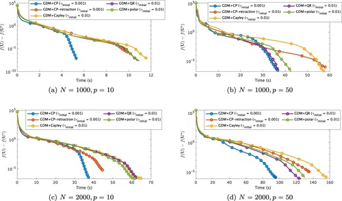
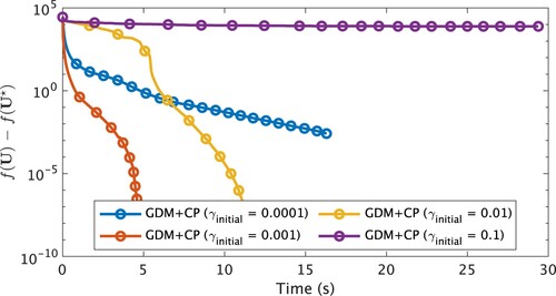
We observe that the proposed GDM+CP reaches the stopping criteria with the shortest CPU time among all five algorithms for every problem size. Possible reasons for the superiority of the proposed Cayley parametrization strategy to the retraction-based strategy are as follows.
The Cayley parametrization strategy exploits the diffeomorphic property of
For Problem 4.1, a global minimizer
As shown in Propositions 2.2 and 3.9, both and
can parameterize respectively open dense subsets of
. However, we observe that (i) the proposed GDM+CP for the minimization of
has faster convergence speed than GDM+CP-retraction for the minimization of
; (ii) the orthogonal feasibility in GDM+CP-retraction deteriorates compared than GDM+CP. We believe that these performance differences are made respectively by (i) the computational complexity for
is more efficient than that of
, and by (ii) calculations of
and
require the Sherman-Morrison-Woodbury formula for matrix inversions in order to achieve comparable computational complexities, and its formula is known to have a numerical instability [Citation22] (see Remark 3.10).
Moreover, although GDM+CP-retraction reaches the stopping criteria without achieving the same level of the final cost value as the others,Footnote9 GDM+CP-retraction has the same or better performance than GDM+Cayley in view of convergence history in Figure at every time. This indicates an efficacy of the parametrization strategy of in the vector space reformulation for Problem 1.1 because GDM+CP-retraction and GDM+Cayley used the same Cayley transform-based retraction.
Finally, we remark that if is set as too large, numerical performance of the proposed GDM+CP can deteriorate because a generated sequence
can go away from
quickly, which induces the insensitivity of
(see Section 3.3). This tendency can be observed from Figure , which illustrates average convergence histories for 10 trials of GDM+CP with each stepsize
in the scenario of Problem 4.1. Figure shows that GDM+CP with
has the best performance among four algorithms. This observation indicates that we need not set
as large for GDM+CP. Not surprisingly, we also see that too small
causes slow convergence speed of GDM+CP with move only a little along
at each iteration.
Figure 3. Convergence histories of GDM+CP with each applied to Problem 4.1 (N = 1000, p = 10) regarding the value
at CPU time for each problem size. Markers are put at every 250 iterations.
4.2. Singular-point issue
In this subsection, we tested how much the singular-points influence the performance of the proposed CP strategy. As we mentioned in Section 3.3, a risk of the slow convergence of Algorithm 1 can arise in a case where a global minimizer of Problem 1.1 is close to the singular-point set
. To see such an influence, we compared CP strategies with several centre point
by a toy Problem 1.1 for the minimization of
with a given
. Clearly, its solution is
.
In this experiment, we used centre points , the global minimizer
and an initial point
, where
is a rotation matrix. From
, we have
. Therefore,
approaches
as
, and
is farthest from
.
We used the stopping criteria (Equation35(35)
(35) ), and parameters
,
, and
for Algorithm 2 to determine a stepsize
.
Table illustrates average results for 10 trials of each algorithm with N = 1000 and p = 10 in this scenario. Figure shows the convergence history of algorithms. The plot shows CPU time on the horizontal axis versus the value on the vertical axis.
Figure 4. Convergence histories of each algorithm applied to Problem 1.1 with , and N = 1000, p = 10 regarding the value
at CPU time. Markers are put at every 250 iterations.
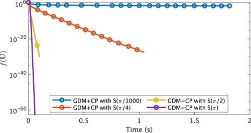
Table 2. Performance of each algorithm applied Problem 1.1 with .
From Figure , we observe that GDM+CP with is the fastest among all algorithms. On the other hand,
generated by GDM+CP with
does not approach a global minimizer
. This implies that the convergence speed of GDM+CP tends to become slower as
, or equivalently as
approaches the singular-point set.
From these observations, the performance of the proposed Algorithm 1 depends heavily on tuning as mentioned in Section 3.3. Since we can not see whether a solution
is distant from
or not in advance before running algorithms, it is desired to circumvent the influence of this singular-point issue. In [Citation38,Citation39], we presented preliminary reports for a CP strategy with an adaptive changing centre point scheme to avoid the singular-point issue by considering Problem 3.8 instead of Problem 1.4.
5. Conclusion
We presented a generalization of the Cayley transform for the Stiefel manifold to parameterize a dense subset of the Stiefel manifold in terms of a single vector space. The proposed Cayley transform is diffeomorphic between a dense subset of the Stiefel manifold and a vector space. Thanks to the diffeomorphic property, we proposed a new reformulation of optimization problem over the Stiefel manifold to transplant optimization techniques designed over a vector space. Numerical experiments have shown that the proposed algorithm outperformed the standard algorithms designed with a retraction on the Stiefel manifold under a simple situation.
Disclosure statement
No potential conflict of interest was reported by the author(s).
Additional information
Funding
Notes
1 is well-defined over
because all eigenvalues of
are pure imaginary. For the second expression in (Equation4
(4)
(4) ), see the beginning of Appendix 3.
2 The closure of is equal to
. For every
, we can approximate it by some sequence
of
with any accuracy, i.e.
.
3 The domain of with
is a subset
of
.
4 As in (Equation9(9)
(9) ),
is the common set
for every
. However, we distinguish
for each
as a parametrization of the particular subset
of
(see also Remark 1.3(b)).
5 Algorithm 1 can serve as a central building block in our further advanced Cayley parametrization strategies, reported partially in [Citation38–40].
6 The local diffeomorphism of around
can be verified with the inverse function theorem and the condition (ii) in Definition B.1.
7 Let be the eigenvalue decomposition with
and a nonnegative-valued diagonal matrix
. From (I2) in Appendix 9, we have
. Thus, we have
.
8 From the relation in Lemma 2.6,
is also a global minimizer of f over
.
9 We note that this early stopping of GDM+CP-retraction can be caused by the instability [Citation22] of the Sherman-Morrison-Woodbury formula used in and
.
10 The subspace is an orthogonal complement to the subspace
with the inner product
. The tangent space
can be decomposed as
with the direct sum ⊕. In view of the orthogonal decomposition, the first term and the second term in the right-hand side of (EquationA1
(A1)
(A1) ) can be regarded respectively as the orthogonal projection of
onto
and
.
11 The exponential mapping at
is defined as a mapping that assigns a given direction
to a point on the geodesic of
with the initial velocity
. The exponential mapping is also a special instance of retractions of
. However, due to its high computational complexity, computationally simpler retractions have been used extensively for Problem 1.1 [Citation1].
References
- Absil PA, Mahony R, Sepulchre R. Optimization algorithms on matrix manifolds. Princeton (NJ): Princeton University Press; 2008.
- Manton JH. Geometry, manifolds, and nonconvex optimization: how geometry can help optimization. IEEE Signal Process Mag. 2020;37(5):109–119.
- Sato H. Riemannian optimization and its applications. Switzerland: Springer International Publishing; 2021.
- Pietersz R, Groenen PJF. Rank reduction of correlation matrices by majorization. Quant Finance. 2004;4(6):649–662.
- Grubišić I, Pietersz R. Efficient rank reduction of correlation matrices. Linear Algebra Appl. 2007;422(2–3):629–653.
- Zhu X. A feasible filter method for the nearest low-rank correlation matrix problem. Numer Algorithms. 2015;69(4):763–784.
- Bai Z, Sleijpen G, van der Vorst H. Nonlinear eigenvalue problems. In: Bai Z, Demmel J, Dongarra J, Ruhe A, van der Vorst H, editors, Templates for the solution of algebraic eigenvalue problems. Philadelphia (PA): SIAM; 2000. p. 281–314.
- Yang C, Meza JC, Wang LW. A constrained optimization algorithm for total energy minimization in electronic structure calculations. J Comput Phys. 2006;217(2):709–721.
- Zhao Z, Bai Z, Jin X. A Riemannian Newton algorithm for nonlinear eigenvalue problems. Comput Optim Appl. 2015;36(2):752–774.
- Zou H, Hastie T, Tibshirani R. Sparse principal component analysis. J Comput Graph Stat. 2006;15(2):265–286.
- Journée M, Nesterov Y, Richtárik P, et al. Generalized power method for sparse principal component analysis. J Mach Learn Res. 2010;11(15):517–553.
- Lu Z, Zhang Y. An augmented Lagrangian approach for sparse principal component analysis. Math Program. 2012;135(1–2):149–193.
- Boufounos PT, Baraniuk RG. 1-bit compressive sensing. In: Annual Conference on Information Sciences and Systems. IEEE; 2008. p. 16–21.
- Laska JN, Wen Z, Yin W, et al. Trust, but verify: fast and accurate signal recovery from 1-bit compressive measurements. IEEE Trans Signal Process. 2011;59(11):5289–5301.
- Joho M, Mathis H. Joint diagonalization of correlation matrices by using gradient methods with application to blind signal separation. In: Sensor Array and Multichannel Signal Processing Workshop Proceedings. IEEE; 2002. p. 273–277.
- Theis FJ, Cason TP, Absil PA. Soft dimension reduction for ICA by joint diagonalization on the Stiefel manifold. In: International Symposium on Independent Component Analysis and Blind Signal Separation. Springer; 2009. p. 354–361.
- Sato H. Riemannian Newton-type methods for joint diagonalization on the Stiefel manifold with application to independent component analysis. Optimization. 2017;66(12):2211–2231.
- Helfrich K, Willmott D, Ye Q. Orthogonal recurrent neural networks with scaled Cayley transform. In: International Conference on Machine Learning. PMLR; Vol. 80; 2018. p. 1969–1978.
- Bansal N, Chen X, Wang Z. Can we gain more from orthogonality regularizations in training deep networks? In: Advances in neural information processing systems. Curran Associates Inc.; 2018. p. 4266–4276.
- Yamada I, Ezaki T. An orthogonal matrix optimization by dual Cayley parametrization technique. In: 4th International Symposium on Independent Component Analysis and Blind, Signal Separation; 2003. p. 35–40.
- Hori G, Tanaka T. Pivoting in Cayley transform-based optimization on orthogonal groups. In: Proceedings of the Second APSIPA Annual Summit and Conference; 2010. p. 181–184.
- Wen Z, Yin W. A feasible method for optimization with orthogonality constraints. Math Program. 2013;142(1–2):397–434.
- Gao B, Liu X, Chen X, et al. A new first-order algorithmic framework for optimization problems with orthogonality constraints. SIAM J Optim. 2018;28(1):302–332.
- Zhu X. A Riemannian conjugate gradient method for optimization on the Stiefel manifold. Comput Optim Appl. 2017;67(1):73–110.
- Zhu X, Sato H. Riemannian conjugate gradient methods with inverse retraction. Comput Optim Appl. 2020;77(3):779–810.
- Fraikin C, Hüper K, Dooren PV. Optimization over the Stiefel manifold. In: Proceedings in Applied Mathematics and Mechanics. Wiley; Vol. 7; 2007.
- Reddi SJ, Hefny A, Sra S, et al. Stochastic variance reduction for nonconvex optimization. In: International Conference on Machine Learning. PMLR; Vol. 48; 2016. p. 314–323.
- Ghadimi S, Lan G. Accelerated gradient methods for nonconvex nonlinear and stochastic programming. Math Program. 2016;156:59–99.
- Allen-Zhu Z. Natasha 2: faster non-convex optimization than SGD. In: Advances in neural information processing systems. Curran Associates Inc.; 2018. p. 2680–2691.
- Ward R, Wu X, Bottou L. AdaGrad stepsizes: sharp convergence over nonconvex landscapes. In: International Conference on Machine Learning. PMLR; Vol. 97; 2019. p. 6677–6686.
- Chen X, Liu S, Sun R, et al. On the convergence of a class of adam-type algorithms for non-convex optimization. arXiv preprint arXiv:1808.02941, 2018.
- Tatarenko T, Touri B. Non-convex distributed optimization. IEEE Trans Automat Control. 2017;62(8):3744–3757.
- Nocedal J, Wright S. Numerical optimization. 2nd ed. New York (NY): Springer; 2006.
- Boumal N, Absil PA. Low-rank matrix completion via preconditioned optimization on the Grassmann manifold. Linear Algebra Appl. 2015;475:200–239.
- Pitaval RA, Dai W, Tirkkonen O. Convergence of gradient descent for low-rank matrix approximation. IEEE Trans Inf Theory. 2015;61(8):4451–4457.
- Sato H, Iwai T. Optimization algorithms on the Grassmann manifold with application to matrix eigenvalue problems. Jpn J Ind Appl Math. 2014;31(2):355–400.
- Xu Y, Zeng T. Fast optimal H2 model reduction algorithms based on Grassmann manifold optimization. Int J Numer Anal Model. 2013;10(4):972–991.
- Kume K, Yamada I. Adaptive localized Cayley parametrization technique for smooth optimization over the Stiefel manifold. In: European Signal Processing Conference. EURASIP; 2019. p. 500–504.
- Kume K, Yamada I. A Nesterov-type acceleration with adaptive localized Cayley parametrization for optimization over the Stiefel manifold. In: European Signal Processing Conference. EURASIP; 2020. p. 2105–2109.
- Kume K, Yamada I. A global Cayley parametrization of Stiefel manifold for direct utilization of optimization mechanisms over vector spaces. In: International Conference on Acoustics, Speech, and Signal Processing. IEEE; 2021. p. 5554–5558.
- Edelman A, Arias TA, Smith ST. The geometry of algorithms with orthogonality constraints. SIAM J Matrix Anal Appl. 1998;20(2):303–353.
- Nikpour M, Manton JH, Hori G. Algorithms on the Stiefel manifold for joint diagonalisation. In: International Conference on Acoustics, Speech, and Signal Processing. IEEE; Vol. 2. 2002. p. 1481–1484.
- Nishimori Y, Akaho S. Learning algorithms utilizing quasi-geodesic flows on the Stiefel manifold. Neurocomputing. 2005;67:106–135.
- Absil PA, Baker CG, Gallivan KA. Trust-region methods on Riemannian manifolds. Found Comut Math. 2007;7(3):303–330.
- Abrudan TE, Eriksson J, Koivunen V. Steepest descent algorithms for optimization under unitary matrix constraint. IEEE Trans Signal Process. 2008;56(3):1134–1147.
- Absil PA, Malick J. Projection-like retractions on matrix manifolds. SIAM J Optim. 2012;22(1):135–158.
- Ring W, Wirth B. Optimization methods on Riemannian manifolds and their application to shape space. SIAM J Optim. 2012;22(2):596–627.
- Huang W, Gallivan KA, Absil PA. A Broyden class of quasi-Newton methods for Riemannian optimization. SIAM J Optim. 2015;25(3):1660–1685.
- Jiang B, Dai YH. A framework of constraint preserving update schemes for optimization on Stiefel manifold. Math Program. 2015;153(2):535–575.
- Manton JH. A framework for generalising the Newton method and other iterative methods from Euclidean space to manifolds. Numer Math. 2015;129:91–125.
- Sato H, Iwai T. A new, globally convergent Riemannian conjugate gradient method. Optimization. 2015;64(4):1011–1031.
- Kasai H, Mishra B. Inexact trust-region algorithms on Riemannian manifolds. In: Advances in neural information processing systems. Curran Associates Inc.; 2018. p. 4254–4265.
- Nesterov Y. A method for solving the convex programming problem with convergence rate o(1/k2). Dokl Akad Nauk SSSR. 1983;269:543–547.
- Siegel JW. Accelerated optimization with orthogonality constraints. J Comput Math. 2020;39(2):207–226.
- Boumal N, Mishra B, Absil PA, et al. Manopt, a Matlab toolbox for optimization on manifolds. J Mach Learn Res. 2014;15:1455–1459.
- Satake I. Linear algebra. New York (NY): Marcel Dekker Inc.; 1975.
- Van den Bos A. Parameter estimation for scientists and engineers. New York (NY): Wiley; 2007.
- Horn RA, Johnson CR. Matrix analysis. 2nd ed. Cambridge (MA): Cambridge University Press; 2012.
Appendix 1.
Basic facts on the Stiefel manifold, the Cayley transform and tools for matrix analysis
In this section, we summarize basic properties on and the Cayley transform together with elementary tools for matrix analysis.
Fact A.1
Stiefel manifold [Citation1,Citation41]
The Stiefel manifold
The dimension of
The Stiefel manifold
The tangent space to
Fact A.2
Commutativity of the Cayley transform pair, e.g. [Citation56]
The Cayley transform φ in (Equation3(3)
(3) ) and its inversion
in (Equation4
(4)
(4) ) can be expressed as
(A2)
(A2)
Fact A.3
Denseness of ; see [Citation20] for
For , define
, i.e.
Then, for
and
defined just after (Equation6
(6)
(6) ),
is a dense subset of
, i.e. the closure of
is
.
Proof.
It suffices to show for that there exists a sequence
such that
.
Let . Then,
can be expressed as
with some
and
(A3)
(A3) (see [Citation56, IV. §5]), where
satisfy
, and
. The relation
ensures
, thus the number
must be even. Define
, where
is given by replacing each diagonal block matrix
in
[in (EquationA3
(A3)
(A3) )] with
. From
for
, we have
and
, which implies
is dense in
.
Lemma A.4
Matrix norms
For
For
For
For
Proof.
(a) Let be the ith column vector of
. Then, it holds
where
stands for the Euclidean norm for vectors. Thus, we have
. By taking the transpose of
in the previous inequality, we have
.
(b) For , let
be the ith largest eigenvalue of a symmetric matrix
. Then, we have the expression
, which asserts
and
.
(c) By (a) and (b), .
(d) The nonsingularity of (see (b)) yields
, and
. Since
is continuous and
is connected,
is a positive-valued.
(e) Let be a singular value decomposition with
and a nonnegative diagonal matrix
. Then, we obtain
, implying thus
by (d). Moreover by (b), we have
and
.
Fact A.5
Derivative of matrix functions (see, e.g. [Citation57, Appendix D])
Let be an open interval. Then, the following hold:
Let
Let
Fact A.6
The Schur complement formula [Citation58, Sec. 0.8.5]
Let be a nonsingular block matrix of
. Define a Schur complement matrix of
by
. Then,
is nonsingular if and only if
is nonsingular, and the inversion
can be expressed as
Moreover, it holds
.
Fact A.7
The Sherman-Morrison-Woodbury formular [Citation58, Sec. 0.7.4]
For nonsingular matrices ,
, and rectangular matrices
,
, let
. If
and
are nonsingular, then
Appendix 2.
Retraction-based strategy for optimization over
We summarize a standard strategy for optimization over .
Definition A.8
Retraction [Citation1]
The set of mappings defined at each
is called a retraction of
if it satisfies (i)
; (ii)
for all
and
.
Retractions serve as certain approximations of the exponential mapping Footnote11. Many examples of retractions for
are known, e.g. with QR decomposition, with polar decomposition and with the Euclidean projection [Citation1,Citation45,Citation46] as well as with the Cayley transform [Citation22,Citation45].
In the view that is a Riemannian manifold, Problem 1.1 has been tackled with retractions as an application of the standard strategies for optimization defined over Riemannian manifold. In such a strategy for
based on a retraction [Citation1,Citation22,Citation24,Citation41–52], the computation for updating the estimate
to
at nth iteration is decomposed into: (i) determine a search direction
; (ii) assign
to a new estimate
. Along this strategy, optimization algorithms designed originally over a single vector space have been extended to those designed over tangent spaces, to
, by using additional tools, e.g. a vector transport [Citation1] and the inversion mapping of retractions [Citation25], if necessary. Such extensions have been made for many schemes, e.g. the gradient descent method [Citation41–43,Citation45], the conjugate gradient method [Citation24,Citation25,Citation47,Citation51], Newton's method [Citation41,Citation50], quasi-Newton's method [Citation47,Citation48], the Barzilai–Borwein method [Citation22,Citation49] and the trust-region method [Citation44,Citation52].
Appendix 3.
Proof of Proposition 2.2
The second equality in (Equation14(14)
(14) ) is verified by
. Fact A.6 and
guarantee the non-singularity of
and
(A4)
(A4) which implies
and the expressions of
in (Equation15
(15)
(15) ).
In the following, we will show on
by dividing 4 steps.
(I) Proof of . For every
, (EquationA2
(A2)
(A2) ) ensures
thus
.
is confirmed by the expression in (Equation15
(15)
(15) ), i.e.
(A5)
(A5) and
.
(II) Proof of . Let
and
in (Equation10
(10)
(10) ). Then, by
we deduce with (Equation15
(15)
(15) )
(III) Proof of . Let
and
with
. It suffices to show
and
. Then, by the definition of
in (Equation10
(10)
(10) ), (Equation11
(11)
(11) ) and (Equation12
(12)
(12) ), and by
each block matrix in (Equation10
(10)
(10) ) can be evaluated as
which implies
.
(IV) Proof of diffeomorphism of and
. From (II) and (III), we have seen
, and both
and
are homeomorphic between their domains and images, and consist of finite numbers of matrix additions, matrix multiplications and matrix inversions, which are all smooth. Therefore,
and
are diffeomorphic between their domains and images.
Appendix 4.
Proof of Theorem 2.3
(a) From the definition of in (Equation6
(6)
(6) ),
is the restriction of
to
, which implies
. Thus, it suffices to show for every
that there exists
satisfying
, which is verified by the following lemma.
Lemma A.9
Let and
with
,
, and
. Define
(A6)
(A6) Then,
and
Proof.
From the skew-symmetries of and
, we have
, thus
.
By letting , Fact A.6 yields
from the non-singularities of
and
(see Lemma A.4(b)). The expressions in (Equation6
(6)
(6) ) and (Equation4
(4)
(4) ) assert that
On the other hand, from (Equation15
(15)
(15) ), we obtain
Clearly to get
, it suffices to show
because
holds automatically by the definition of
in (EquationA6
(A6)
(A6) ). The equation
is verified by
and by
(b) (Openness) By the continuity of , the preimage
is closed on
. Since
is closed in
,
is open in
.
(Denseness) It suffices to show, for every , there exists a sequence
such that
. Let
with
, where
satisfies
. Then,
(see (a)) ensures
. By using the denseness of
in
(see Fact A.3), we can construct a sequence
such that
. Moreover by defining
, the continuity of Ξ yields
.
(c) are open dense subsets of
from Theorem 2.3(b). The openness of
is clear. To show the denseness of
in
, choose
and
arbitrarily. By the open denseness of
, there exist
and
satisfying
, where
. The denseness of
in
yields the existence of
, from which we obtain
.
(d) From (EquationA5(A5)
(A5) ), we have
for
, where
is the Schur complement matrix of
. Fact A.6 yields
due to
. Lemma A.4(d) ensures
. By Lemma A.4(e), we have
as
, implying thus
.
Assume that satisfies
. By
in Lemma A.4(e), we have
. The assumption asserts
as
.
Appendix 5.
On the choice of for in Proposition thm2.2
For 2p<N, let and
satisfy
, and
. From
, we have
(A7)
(A7) From
, Theorem 2.3(a) ensures
.
In the following, let us consider the case of to show that
is not injective on
. Since
does not depend on
, we can assume, without loss of generality,
,
and
with
and
satisfying
. We have
(A8)
(A8)
Now, by using , define
as
and
, where
is guaranteed by
and 0<N−2p. Then,
and (EquationA8
(A8)
(A8) ) with
yield
(A9)
(A9) where
,
and
Finally, by applying Lemma A.9 to (EquationA9(A9)
(A9) ) and (EquationA7
(A7)
(A7) ), we deduce
for all
. This implies that infinitely many
achieve
, and clearly
is not injective.
Appendix 6.
Proof of Proposition 2.9
The differentiability of is verified by the differentiabilities of f and
. Let
. From the chain rule, we obtain
Moreover, by
and Fact A.5, we deduce
Therefore, we have
where
is defined in (Equation22
(22)
(22) ). Furthermore, we have
, where the first equality follows by
for any symmetric matrix
and the second equality follows by (Equation21
(21)
(21) ) and
. Therefore, we obtain
(A10)
(A10)
On the other hand, by letting be the gradient of
at
, it follows
(A11)
(A11) By noting
, (EquationA10
(A10)
(A10) ) and (EquationA11
(A11)
(A11) ) imply
. By applying (EquationA4
(A4)
(A4) ) to (Equation22
(22)
(22) ), the expression (Equation23
(23)
(23) ) is derived as
By substituting into (Equation22
(22)
(22) ), and by
, we deduce
and
Appendix 7.
Proof of Proposition 2.10
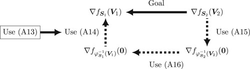
(I) Proof of Proposition 2.10(a). We need the following lemma to show Proposition 2.10(a). Figure illustrates the relation between the following lemma and Proposition 2.10(a).
Figure A1. A flow chart represents the overview of the proof of Proposition 2.10(a). The goal is to derive a transformation formula from to
under
.
Lemma A.10
Let be a differentiable function, and let
,
and
in (Equation6
(6)
(6) ), implying thus
. Then, the following hold:
For
The gradients of
If
Proof.
(a) Combining and
, we obtain
(A17)
(A17) The relation (EquationA13
(A13)
(A13) ) is obtained by substituting (EquationA17
(A17)
(A17) ) to an alternative expression of (Equation21
(21)
(21) ):
(b) (EquationA14(A14)
(A14) ) is confirmed by applying (EquationA13
(A13)
(A13) ) to (Equation20
(20)
(20) ) as
To derive (EquationA15(A15)
(A15) ) from (EquationA14
(A14)
(A14) ), let first
and apply (EquationA4
(A4)
(A4) ) with
as
(A18)
(A18) where
satisfies
. By substituting (EquationA18
(A18)
(A18) ) to (EquationA14
(A14)
(A14) ), we obtain
and
from which we obtain
(c) From , and
we see
and
by
.
Thus, it follows from and
that
Return to the proof of Proposition 2.10(a). Let and
. Since
, Lemma A.10(c) implies
. Moreover from Lemma A.10, we have the relations
Finally by substituting the second and last relations into the first relation, we complete the proof.
(II) Proof of Proposition 2.10(b) and (c). From Proposition 2.10(a), Lemma A.4(a) and (b), we obtain
where the last inequality is derived by
from the fact that each eigenvalue of a triangular matrix equals its diagonal entry. Finally by applying Lemma A.4(b) again, we obtain Proposition 2.10(b), which implies Proposition 2.10(c).
Appendix 8.
Useful properties of for optimization
The properties of in the following Proposition A.11 are useful in transplanting powerful computational arts designed for optimization over a vector space into the minimization of
over
. Indeed, the Lipschitz continuity of the gradient is one of the commonly used assumptions in optimization over a vector space (see, e.g. [Citation27–32]). The boundedness of the gradient is a key property for distributed optimization and stochastic optimization over a vector space (see, e.g. [Citation30–32]). The variance bounded of the gradient is also commonly assumed in stochastic optimization over a vector space (see, e.g. [Citation28–30]).
Proposition A.11
Bounds for gradient after Cayley parametrizaton
Let be continuously differentiable. Then, for any
, the following hold:
(Lipschitz continuity). If
(Boundedness).
(Variance boundedness). Suppose
Proof.
The existence of the maximum of over
is guaranteed by the compactness of
and the continuities of
and
. We divide the proof of (a)–(c) as follows. Recall that
and
for
were respectively defined as (Equation22
(22)
(22) ) and (Equation21
(21)
(21) ), and we have
(see Proposition 2.9). In the following, we use properties of
; (i)
for
; (ii) the linearity of
.
(I) Proof of Proposition A.11(a). First, we introduce a useful inequalities.
Lemma A.12
Lipschitz continuity of
For every ,
is Lipschitz continuous over
with a constant 2, i.e.
Proof.
From (Equation14(14)
(14) ) and Lemma A.4(a) and (c), we have
Return to the proof of Proposition A.11(a). From (Equation20(20)
(20) ), (Equation21
(21)
(21) ) in Proposition 2.9, we have
(A22)
(A22) Moreover, from (Equation22
(22)
(22) ), for all
with
, we deduce
(A23)
(A23) The first term in the right-hand side of (EquationA23
(A23)
(A23) ) can be bounded as
Similarly the last term in (EquationA23
(A23)
(A23) ) can be bounded above by
. The second term in (EquationA23
(A23)
(A23) ) can be evaluated as
Therefore, the left-hand side of (EquationA23
(A23)
(A23) ) is bounded as
which is combined with (EquationA22
(A22)
(A22) ) to get (EquationA19
(A19)
(A19) ).
(II) Proof of Proposition A.11(b). From (Equation20(20)
(20) ), (Equation21
(21)
(21) ) in Proposition 2.9, we have
By using Lemma A.4(a) and (b), we get
which implies (EquationA20
(A20)
(A20) ).
(III) Proof of Proposition A.11 A.11. From (Equation20(20)
(20) ), (Equation21
(21)
(21) ) in Proposition 2.9, we obtain, for each ξ,
By taking the expectation of both sides, we get (EquationA21
(A21)
(A21) ).
Appendix 9.
Proof of Proposition 3.7
Application of (Equation14(14)
(14) ) to
yields
(for the 2nd equality, see the proof of Lemma A.4(c)) and
where
, the second last inequality is derived by Lemma A.4(b), and the last inequality is derived by (EquationA4
(A4)
(A4) ).
To evaluate the norm , let
be the eigenvalue decomposition, where
is an orthogonal matrix and
is a diagonal matrix whose entries are non-negative. Then, we have
The norm
is bounded above as
(A25)
(A25) where the last inequality is derived from the skew-symmetry of
and Lemma A.4(b). Moreover, by
, we have
. Furthermore, from the definition of the spectral norm, we have
. By substituting these relations into (EquationA24
), we completed the proof of (Equation28
(28)
(28) ). The equation (Equation29
(29)
(29) ) is verified by
.
Appendix 10.
Gradient of
Proposition A.13
Let and
satisfy
. For a differentiable function
, the Cayley transform-based retraction
in (Equation30
(30)
(30) ), and
, the function
is differentiable with
where
and
. The matrix
can be expressed as
with
and
.
Proof.
Let . From the chain rule and Fact A.5, we obtain
(A26)
(A26) due to
(see (Equation30
(30)
(30) ) and (Equation4
(4)
(4) )) and
For
, we have
because
is skew-symmetric. Fact A.1(d) yields
.
On the other hand, we obtain
(A27)
(A27) From (EquationA26
(A26)
(A26) ), (EquationA27
(A27)
(A27) ) and
, it holds
.
In the following, let us consider the expression of along the discussion in [Citation22, Lemma 4]. From
, we have
. Then, applying the Sherman-Morrison-Woodbury formula (see Fact A.7) to
, we obtain
.