Relating hydrograph components to rainfall and streamflow: a case study from northern Taiwan

Abstract

This study investigates the characteristics of hydrograph components from a watershed in Taiwan. Hydrograph components were modelled by using a model of three serial reservoirs with one parallel reservoir. Mean rainfall was calculated by using the block kriging method. The model parameters for 38 events were calibrated by using the shuffled complex evolution optimization algorithm. The model verification was made using 18 events. Based on the study results, the following findings were obtained: (1) for single-peak events, times to peak of hydrograph components are an increasing power function of the peak time of rainfall; (2) peak discharges of hydrograph components are linearly proportional to that of total runoff, and the ratios of quick and slow runoff are approximately 83% and 17% of total runoff, respectively; and (3) the total volume of quick runoff component is 52% of total runoff and that of slow runoff is 27%.

Editor D. Koutsoyiannis

Citation Li, Y.-J., Cheng, S.-J. Pao, T.-L. and Bi, Y.-J., 2012. Relating hydrograph components to rainfall and streamflow: a case study from northern Taiwan. Hydrological Sciences Journal, 57 (5), 861–877.

Résumé

Cette étude s'intéresse aux caractéristiques des composantes de l'hydrogramme d'un bassin versant à Taïwan. Les composantes de l'hydrogramme ont été modélisées en utilisant un modèle de trois réservoirs en série avec un réservoir en parallèle. La pluviométrie moyenne a été calculée en utilisant la méthode du krigeage par blocs. Les paramètres du modèle pour 38 événements ont été calés à l'aide de l'algorithme optimal « shuffled complex evolution ». La vérification du modèle a été réalisée en utilisant 18 événements. Sur la base des résultats analytiques, on a trouvé que: (1) pour des événements à pointe unique, les temps de montée des composantes de l'hydrogramme sont corrélés avec le temps de montée des précipitations selon une loi de puissance croissante; (2) les débits de pointe des composantes de l'hydrogramme sont linéairement proportionnels à ceux du ruissellement total, le rapport étant approximativement de 83% pour un ruissellement rapide et de 17% pour un écoulement lent; et (3) les relations des débits totaux ont des rapports directs entre les composantes de l'hydrogramme et les ruissellements totaux observés, de 52% pour un ruissellement rapide et de 27% pour un écoulement lent.

Key words:

• block kriging
• linear cascade reservoir
• streamflow components
• hydrograph shape
• runoff characteristics

Mots clefs:

• krigeage par bloc
• réservoirs en cascade linéaire
• composantes du débit
• forme de l'hydrogramme
• caractéristiques du ruissellement

INTRODUCTION

In developing conceptual rainfall–runoff models it is convenient to use approximations of the convolution integral to derive the models and to generate the outlet runoff of a watershed. These models, which are derived from a convolution integral, are generally known as unit hydrograph (UH)-based models and include: the Nash model (Nash 1957); Clarke's model (Clarke 1973, Ahmad et al. 2009); the geomorphologic instantaneous unit hydrograph (GIUH) (Jin 1992, Franchini and O'Connell 1996, Nourani et al. 2009), the distributed parallel model (Hsieh and Wang 1999), and sub-watershed divisions (Agirre et al. 2005). Rainfall–runoff modelling with IUHs has been studied by O'Connell and Todini (1996), Melone et al. (1998), Bhadra et al. (2010) and others. Furthermore, the changes in hydrograph characteristics on an urbanized watershed have also been evaluated by identifying the relationships between IUH parameters and urbanization variables (Cheng and Wang 2002, Cheng et al. 2008b, 2010, Huang et al. 2008a, 2008b, Kliment and Matoušková 2009).

The essential input of UH-based models such as the Nash model are usually recordings of rainfall and streamflow. The application of models that are based on the IUH theory involves determining both the effective rainfall and the baseflow of a rainfall–runoff event in advance. The baseflow, which is computed separately from the direct runoff, is a streamflow component, and is frequently considered a constant in a rainfall–runoff event. Effective rainfall is the total rainfall, after deducting the rainfall lost to depression storage, interception, evaporation and infiltration. Various studies have addressed the effects of different methods for estimating rainfall excess and baseflow on the accuracy of modelling surface runoff (Mays and Taur 1982, Cheng and Wang 2002). Prior to development of the IHACRES (Jakeman et al. 1990, Jakeman and Hornberger 1993) and Tank models (Sugawara 1979, 1995, Madsen 2000, Yue and Hashino 2000, Hashino et al. 2002, Chen et al. 2003, Lee and Singh 2005), hydrological modelling frequently focused on generating direct runoff by a linear convolution with the specific input–output structures.

Hydrological modelling conveniently considers watersheds in terms of a cascade of linear reservoirs. The cascade assumption has been used for decades to conceptually describe the catchment response to excess rainfall. The output of an upstream reservoir becomes the input to the next reservoir downstream, and the model behaviour is governed by two parameters, as in the Nash model (Nash 1957). The IHACRES model has a linear module, which allows any configuration of stores in parallel or in series. This linear module is defined as a recursive relationship at a time step for generating streamflow, calculated as a linear combination of its antecedent values and excess rainfall. In this linear combination, the optimal configuration of two parallel storages in the linear routing module is frequently used to generate streamflow components. The IHACRES model has numerous variants, such as CMD-IHACRES (Schreider et al. 2002, Evans 2003, Croke et al. 2006, Carcano et al. 2008) and IHAC (Andréassian et al. 2001). These studies identify separate UHs for relatively quick- and slow-response components of streamflow, resulting in a continuous hydrograph separation. The Tank model is represented by a cascade of conceptual tanks, and the whole period is divided into sub-periods, in which each of the components plays the main part. The volume and shape are calculated in each sub-period, and are used for the adjustment of the respective tanks. The Tank model is composed of two types of tank, which can be approximated by a linear model by moving the side outlets or outlet to the bottom. Such complex cascade models generally have many parameters related to catchment characteristics, for example, the IHACRES model requires between five and seven parameters to be calibrated and the Tank model at least eight. Linear cascade models have several practical applications in hydrology, such as estimating a runoff hydrograph at the catchment outlet.

The assumptions of the IUH, such as the Nash-type linear reservoirs, were preserved for the model used in this study (that is, a uniform spatial distribution of rainfall and the principle of linear superposition). The model structure consists of a serial cascade of three linear reservoirs, with one in parallel. Each linear reservoir has a kernel function with an exponential expression derived from the equation of continuity and the convolution integral. The exponential expressions were used to illustrate the storage status of each linear reservoir during the rainfall–runoff process. Generating hydrograph components in a specific river during a storm is the first application of the proposed model, with hydrological serial and parallel cascades. The causal relationships among rainfall, total runoff observations and generated runoff components are discussed. The block kriging method was used to estimate the mean rainfall as the input for the model. The rate coefficients of each outlet in the three serial reservoirs with one in parallel were defined as specific parameters, which were acquired through an optimization approach. In the optimization process, three evaluated criteria and an objective function were used to compare the simulations and observations of the total runoff hydrographs. The representative parameters are proportional to the magnitudes of the outlets and were used to determine surface runoff, rapid subsurface runoff, delayed subsurface runoff and groundwater runoff. Finally, the hydrograph components (quick and slow flows) of the research watershed outlet and their characteristics in comparison to observations of rainfall and total runoff are discussed.

THE BLOCK KRIGING METHOD

The block kriging method was used to estimate the hourly, spatially-uniform rainfall over the study watershed. Variogram identification (Lebel and Bastin 1985) is an essential process before using the kriging approach. The kriging approach has several applications in various research fields, especially for the design of raingauge networks (Bastin et al. 1984, Cheng et al. 2008a), raingauge significance evaluation (Cheng 2011), spatial interpolation of rainfall (Goovaerts 2000, Syed et al. 2003) and space–time rainfall interpolation (Cheng et al. 2007). The kriging method is theoretically superior to the Thiessen method, as the former allows the uncertainty in interpolated estimates to be calculated.

Climatological mean semivariogram

The set of time sequences of discontinuous point-rainfall depths with time period p(t, x) can be considered as a realization of two-dimensional random fields. Considering n raingauges in a river basin, for each time period t, a realization π(t) of the random n vectors can be expressed as:

(1)

A basic semivariogram, the scaled climatological mean semivariogram, proposed by Bastin et al. (1984), was established through dimensionless rainfall data on a project basin (Cheng et al. 2007). The relationship between the hourly semivariogram, γ(t, h_ij ), and the scaled climatological mean semivariogram, (h_ij , a), is given as:

(2)

where h_ij represents the distance between arbitrary raingauges x_i and x_j (m); ω(t) denotes the sill of the semivariogram for time period t (mm²) and is time-variant; a represents the range of the scaled climatological mean semivariogram (m) and is time-invariant; and s(t) denotes the standard deviation (mm) of rainfall of all raingauges for time period t. The empirical semivariogram is expressed as:

(3)

The empirical experimental semivariogram can be calculated by using equation (3)(3), but as it is computed from discontinuous point-observations (i.e. rainfall depth recordings of scattered raingauges), it is not spatially continuous. A realistic application for the block kriging method is to use a semivariogram model to obtain spatial continuity of rainfall variations.

Block kriging system

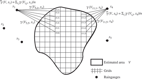
The block kriging method obtains optimal weights by assuming a given spatial structure of rainfall. The system (equation (4)(4)) is derived by applying Lagrange's multipliers, and the estimated area V must be divided into M grid cells before the hourly mean rainfall of storm events over the watershed is calculated:

(4)

where γ(x_i , x_j ) is the semivariogram of raingauges x_i and x_j (mm²); V_m is the mth grid in the estimated area; γ(V_m , x_i ) represents the semivariogram of the mth grid V_m and raingauge x_i (mm²); and λ_i is the weighting of each raingauge. Figure 1 shows the computation procedure of the mean semivariogram, , between the grid cells of the area and raingauges.

Fig. 1 Computation of the mean semivariogram between the grid cells of the area and raingauges.

CASCADE OF LINEAR RESERVOIRS MODEL

The model in this study is constructed from three serial linear reservoirs with one in parallel. The individual reservoirs are viewed as independent systems that follow the hydrological cycle, i.e. the inputs and outputs of the linear systems are analogous to natural flows such as runoff components and infiltration. The convolution integral is used to describe the interior transformations of independent systems for the inputs and outputs.

Structure and flow mechanism within the model

The proposed model is a lumped rainfall–runoff model for single input and multiple outputs. Average rainfall is the single input for the whole model system, while the outputs are surface runoff, subsurface runoff and groundwater runoff at the watershed outlet. Subsurface runoff is divided into rapid and delayed components: rapid subsurface runoff is water flowing into the soil layer near the surface, while delayed subsurface runoff is flow that is distant from the infiltration surface. Furthermore, surface runoff is also denoted as quick runoff, while slow runoff is the sum of subsurface runoff and groundwater runoff. Hence, the structure of the model comprises three serial linear reservoirs with one in parallel, as derived by Yue and Hashino (2000). The model structure is shown in Fig. 2.

Fig. 2 The model structure of three serial cascaded linear reservoirs with one in parallel.

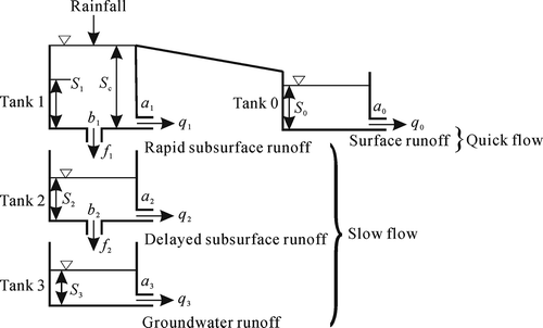
The upper and middle reservoirs in the series (Tanks 1 and 2, Fig. 2) both have one horizontal and one vertical opening, while the parallel reservoir (Tank 0) and the lowest serial reservoir (Tank 3) only have a horizontal opening. The rates at which water moves through the horizontal openings of the parallel and serial reservoirs are denoted a ₀, a ₁, a ₂ and a ₃, respectively while the vertical openings in the upper and middle reservoirs in series are denoted b ₁ and b ₂, respectively. The flow discharges, q ₁, q ₂ and q ₃, of the horizontal openings at the bottom of the three serial reservoirs are modelled as a rapid subsurface runoff, delayed subsurface runoff and groundwater runoff, respectively. The flow analogous to surface runoff is indicated by q ₀ at the horizontal opening of the parallel reservoir, which occurs when storage in the upper reservoir in the series is higher than the height, S_c , which describes the antecedent soil moisture before rainfall. The infiltration amount f ₁ flows via the vertical hole in the upper reservoir to the middle reservoir in the series, and discharge f ₂ represents the amount of percolation originating from the deep soil aquifer, flowing from the middle to the lowest serial reservoir.

Rainfall, r, first falls into the upper reservoir (Tank 1), which begins to store this rainwater (i.e. S ₁ > 0). The rapid subsurface runoff q ₁ and infiltration f ₁ are simultaneously produced and flow out of the upper reservoir. When the storage height of the upper reservoir exceeds S_c (Tank 1 is full), overflow occurs to the parallel reservoir (Tank 0), and surface runoff q ₀ is generated (i.e. S ₁ > S_c ). Infiltration f ₁ enters the middle serial reservoir (Tank 2) and is stored until the delayed subsurface runoff, q ₂, and percolation, f ₂, start flowing (S ₂ > 0). Finally, percolation, f ₂, flows into the lowest serial reservoir (Tank 3), and its storage status is the same as that in Tank 2; then groundwater, q ₃, flows from the lowest serial reservoir.

Storage functions over time

According to the flow mechanism of the model, runoff components q ₁, q ₂ and q ₃, infiltration f ₁ and percolation f ₂ are storage functions of three serial reservoirs, whereas surface runoff q ₀ is the amount that overflows from the upper serial reservoir into and out of the parallel reservoir. The outflows, excluding q ₀, are expressed (in mm/h) as:

(5)

(6)

Each reservoir in this study is considered as an independent input–output system; therefore, each satisfies the equation of continuity:

(7)

where I, Q and S denote input, output and storage, respectively. By combining equation (7)(7) and the convolution integral, the storage functions can be obtained from specific inputs of the model based on the IUH. Assuming the input of the upper reservoir is the rainfall that occurred between 0 and Δt (which depends on the recording interval for the rainfall data; 1 hour in this study), I ₁(t) = 1/Δt, and that of the other time periods is zero, then, the storage, S ₁(t), which is less than S_c , for the upper serial reservoir can be derived as:

(8)

(9)

where C ₁ = a ₁ + b ₁. Similarly, the input I ₂(t) of the middle serial reservoir is the infiltration output f ₁(t) of the upper serial reservoir (i.e. I ₂(t) = f ₁(t) = b ₁ S ₁(t)), the storage S ₂(t) for the middle serial reservoir is derived as follows:

(10)

(11)

where C ₂ = a ₂ + b ₂. Finally, the input of the lowest reservoir in serial is I ₃(t) = f ₂(t) = b ₂ S ₂(t)), the mathematical expression of storage height S ₃(t) of the lowest reservoir in serial is expressed as:

(12)

(13)

Similar to the upper serial reservoir (Tank 1), for unit input I ₀ = 1 and duration Δt, the unit pulse response function of the parallel reservoir, used to generate surface runoff, q ₀, may be obtained as:

(14)

(15)

Parameter constraints

Based on the physical characteristics of the hydrological cycle and conceptual considerations on soil infiltration and runoff generation, the model parameters should be constrained by the following eight inequalities:

1.	: rate of surface runoff q 0 should be larger than that of rapid subsurface runoff q 1;
2.	: rate of rapid subsurface runoff q 1 is larger than that of delayed subsurface runoff q 2;
3.	: rate of delayed subsurface runoff q 2 is larger than groundwater amount q 3;
4.	: rate of infiltration resulting from the upper reservoir should be larger than that of percolation f 2 coming from the middle reservoir;
5.	: sum of two opening ratios in the upper reservoir in the series should be less than or equal to 1;
6.	: sum of two opening ratios in the middle reservoir in the series is less than or equal to 1;
7.	: the opening ratio of the lowest reservoir in serial is less than or equal to 1; and
8.	: the opening ratio of the parallel reservoir is less than or equal to 1.

PARAMETER OPTIMIZATION AND EVALUATION CRITERIA

Objective function

When optimizing the parameters, an objective function must be assigned, and this is used to minimize error between simulations and observations of the runoff hydrographs. The following expression (Yue and Hashino 2000) was used for parameter optimization:

(16)

where F _obj is the value of the objective function; T is the total duration of the observed hydrograph; Q _obs(t) is the observed value of the runoff hydrograph at time period t; and Q _est(t) is the simulated value at time period t.

Evaluation criteria

Three criteria were used to evaluate the suitability of the rainfall–runoff model for the basin of interest: the coefficient of efficiency (CE, Nash and Sutcliffe 1970; Nayak et al. 2005); the error of peak discharge (EQ _p ); and the error of the time to peak (ET _p ). The CE is commonly used as a measure of model performance.

Peak discharge and time to peak are also important characteristics of flood hydrographs. Hence, differences in peak quantity and time to peak between observations and simulations were also examined herein. The EQ _p and ET _p have also been frequently used to examine simulated results (Chen et al. 2003, Moramarco et al. 2005). The evaluation criteria are calculated as follows:

Coefficient of efficiency:

(17)

where is the average discharge of the observed hydrograph. The better the fit, the closer CE is to one. A negative value for CE means that model predictions are worse than predictions using a constant that is equal to the average observed value.

Error of peak discharge (%):

(18)

where Q _est,p is the peak discharge of the simulated hydrograph and Q _obs,p is the peak discharge of the observed hydrograph.

Error of time to peak:

(19)

where T _est,p is the time for the simulated hydrograph peak to arrive and T _obs,p is the time required for the observed hydrograph peak to arrive.

WATERSHED DESCRIPTION

Geographical features

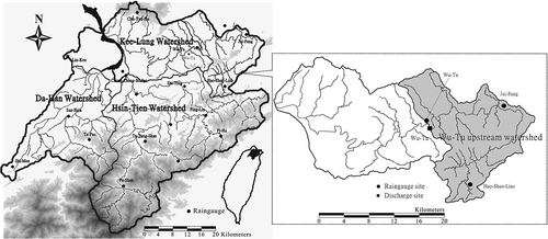
The upstream area of the Wu-Tu watershed was chosen to explore the characteristics of the modelled runoff components in the research area. The watershed surrounds Taipei city in the northern part of Taiwan (Fig. 3). The Wu-Tu watershed covers about 204 km², and the mean annual precipitation and runoff depth are 2865 and 2177 mm, respectively. Due to the rugged topography of the watershed, runoff pathlines are short and steep, and rainfall is not uniform in terms of both time and space. Large floods arrive rapidly in the middle-to-downstream reaches of the watershed, causing serious damage during summers.

Fig. 3 Location maps of the Tamshui River basin and the Wu-Tu watershed, in Taiwan.

Data studied

There are three raingauges (Jui-Fang, Wu-Tu and Huo-Shao-Liao) and one discharge measurement site (Wu-Tu) on the upstream portion of the Wu-Tu watershed. The 56 recorded rainfall–runoff events of 1966–2008 were used as the study sample. This sample includes 11 multi-peak events, the remaining ones being single-peak events. In total, 38 events (five multi-peak events) were selected for parameter calibration, and the remaining 18 (six multi-peak events) were used to verify the applicability of the calibrated parameters. The spatial variations of rainfall (i.e. semivariogram in the block kriging method) were analysed using the data from the 14 raingauges (including those at Jui-Fang, Wu-Tu and Huo-Shao-Liao) (Fig. 3) located in and around the upstream portion of the Wu-Tu watershed. Hourly inputs of mean rainfall for the model were estimated using the analysed semivariogram, kriging system and three raingauges (i.e. Jui-Fang, Wu-Tu and Huo-Shao-Liao) located in the Wu-Tu watershed.

RESULTS AND DISCUSSION

The primary goal of this study was to explore the hydrograph characteristics of runoff components in a river by simulating streamflow hydrographs and their components. Translating a single input (rainfall) into a multi-output result (streamflow components) depends on the lumped model of three serial and one parallel reservoirs. Traditionally, streamflow components during a rainfall–runoff event are divided into several components, including surface runoff, rapid subsurface runoff, delayed subsurface runoff and groundwater. The characteristics of quick and slow flows related to rainfall observations and observed total runoff hydrographs were also explored in this study. Based on the analytical results, the model applicability and variation of the calibrated parameters were evaluated, and simulations were applied for water resource planning in the research area. The runoff characteristics that are compared include the time to peak, peak discharge and total discharge.

Hourly mean rainfall

The hourly rainfall semivariogram is a function of time , but a time average form was taken for non-zero recordings in time interval, T. The analysis of the scaled climatological mean semivariogram for the 56 rainfall events, recorded by 14 raingauges in or around the watershed, was completed. The power form (Fig. 4) was then applied for fitting as follows:

(20)

Fig. 4 Scaled climatological mean semivariogram in the Wu-Tu watershed.

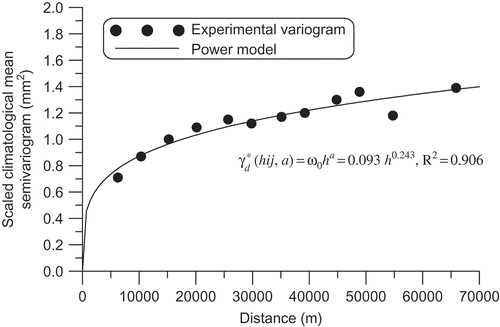
where ω₀ denotes the scale parameter of the scaled climatological mean semivariogram (mm²). Variance s ²(t) of a realization π(t) for each time period t can be calculated from the hourly rainfall measurements. Hourly semivariograms of rainfall events can then be directly calculated using equations (2)(2) and (20).

The estimated area must be divided into M grids before calculating the hourly mean rainfall during storm events over the watershed by applying equation (4)(4). The estimated area was divided into 2665 × 1-km² grids. This study used observations from three raingauges located in the Wu-Tu watershed to estimate the hourly mean rainfall for applying to the calibrated and verified events.

Parameter calibration

In the processes of translating the rainfall runoff, the model parameters for each event were determined by using the shuffled complex evolution (SCE) optimal algorithm (Duan et al. 1993). These calibrated parameters reflect the complex rainfall–runoff processes resulting from the watershed and the meteorological characteristics of each case at that time. They also reflect errors in the rainfall estimates, initial conditions and observed flow. Table 1 shows the comparisons of the simulated and observed runoff hydrographs by using the three criteria (CE, EQ _p and ET _p ). Figure 5 shows the plot of four simulation results in 38 calibrated rainfall–runoff events for quick and slow runoff hydrographs.

Table 1  Calibration results for the model of three serial reservoirs with one parallel reservoir

Event name (date)	CE	EQ p	ET p	Shape*
		(%)	(h)
Typhoon Cora (1966-09-06)	0.95	15.47	0	S
Typhoon Betty (1972-08-16)	0.97	−0.88	−1	S
Typhoon Billie (1976-08-09)	0.98	−9.01	1	S
Typhoon Vera (1977-07-31)	0.81	33.86	0	S
Typhoon Ora (1978-10-12)	0.79	23.08	−2	M
Typhoon Irving (1979-08-14)	0.94	18.97	0	S
Storm (1980-11-19)	0.87	18.61	0	S
Typhoon Andy (1982-07-29)	0.77	15.90	0	S
Typhoon Cecil (1982-08-09)	0.80	17.71	0	M
Storm (1983-10-12)	0.96	7.54	1	S
Storm (1983-10-14)	0.99	−5.74	0	S
Storm (1984-06-02)	0.94	−29.21	0	S
Storm (1984-11-18)	0.85	13.01	2	S
Typhoon Nelson (1985-08-22)	0.91	−2.56	0	S
Typhoon Alex (1987-07-27)	0.88	−5.92	2	S
Typhoon Abe (1990-08-30)	0.76	11.36	−1	S
Storm (1990-09-01)	0.92	−4.66	0	S
Storm (1990-09-02)	0.92	−16.23	2	S
Storm (1994-06-18)	0.85	−16.67	0	S
Typhoon Fred (1994-08-20)	0.93	15.31	2	S
Typhoon Gladys (1994-09-01)	0.91	−17.05	2	S
Typhoon Herb (1996-07-31)	0.95	6.23	1	S
Typhoon Winnie (1997-08-17)	0.79	−2.12	0	S
Typhoon Amber (1997-08-29)	0.75	26.26	1	S
Storm (1999-09-26)	0.82	−11.56	4	S
Typhoon Bebinca (2000-11-08)	0.68	12.79	0	M
Typhoon Rananim (2004-08-12)	0.61	−8.16	1	M
Storm (2004-08-17)	0.87	−13.36	2	S
Storm (2004-10-01)	0.79	12.78	2	S
Storm (2005-05-09)	0.78	26.76	1	S
Storm (2005-09-10)	0.76	−4.62	3	S
Storm (2005-12-04)	0.88	1.44	3	S
Storm (2005-12-11)	0.70	17.90	5	S
Storm (2006-06-06)	0.85	10.57	4	M
Storm (2007-06-15)	0.94	−28.79	1	S
Storm (2007-09-04)	0.94	−18.36	1	S
Storm (2008-05-30)	0.72	−13.62	1	S
Storm (2008-10-10)	0.87	8.55	1	S
Mean	0.85	2.78	1.03
Note: *S represents a single-peak rainfall event and M represents a multi-peak rainfall event.

Fig. 5 Calibration of runoff hydrographs for rainfall–runoff events.

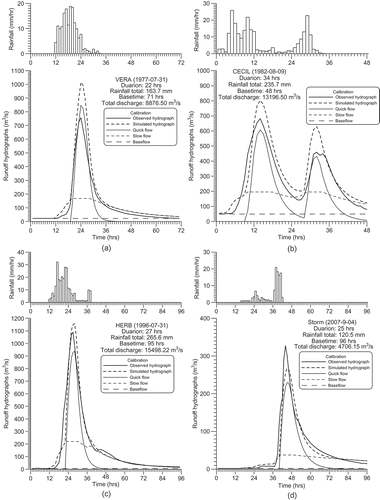
Regarding CE for model calibration, in 25 calibrated events it exceeds 0.8, in 11 cases it lies within [0.7–0.8], and in only one case it is below 0.7 (Table 1). With regard to EQ _p , in all samples it is smaller than 20%, except for six typhoons/storms. The ET _p values are less than or equal to 3 h; while in three events they are longer than 3 h. The average values of the three criteria CE, EQ _p and ET _p are 0.85, 2.78% and 1.03 h, respectively. This comparison also demonstrates that the calibration is satisfactory for regenerating rainfall–runoff processes. Model calibration using the three evaluation criteria demonstrates that the calibrated parameters are able to illustrate the situation of the studied watershed during rainfall–runoff processes.

Variations of calibrated parameters

Table 2 lists the estimated values of the seven model parameters for 38 calibrations. Parameter S_c represents the antecedent soil condition before a storm/typhoon event, and varies within a large range between a maximum of 210.94 mm and a minimum of 3.83 mm with a standard deviation of 48.25 mm. An antecedent value of a storm depends on the time interval between a storm and the previous storm. This indicates that the antecedent value for one storm may differ markedly from that for another. The rate coefficient, a ₀, of surface runoff is spread over a range of 1.0000–0.0588, with a standard deviation of 0.2664. The varied extent of a ₀ is also as large as that for the antecedent condition, as the generation of surface runoff is controlled by topography, characteristics of the surface soil layer (for example antecedent soil moisture, infiltration rate and land use), and weather factors (for example rainfall intensity). As the complexity of the natural flow generation mechanism increases, the range of its corresponding parameter increases due to several unknown/uncontrolled causes.

Table 2  The estimated values of the model parameters between 38 calibrations

Event name (date)	Sc	a 0	a 1	a 2	a 3	b 1	b 2
Typhoon Cora (1966-09-06)	94.83	0.4227	0.0268	0.0001	0.0001	0.0268	0.0001
Typhoon Betty (1972-08-16)	22.45	0.1265	0.1265	0.0051	0.0051	0.1265	0.0001
Typhoon Billie (1976-08-09)	68.77	0.2968	0.0060	0.0001	0.0001	0.0060	0.0001
Typhoon Vera (1977-07-31)	89.97	0.4706	0.0287	0.0001	0.0001	0.0287	0.0001
Typhoon Ora (1978-10-12)	11.40	0.2779	0.2779	0.2743	0.1208	0.2779	0.2741
Typhoon Irving (1979-08-14)	54.59	0.1879	0.0841	0.0001	0.0001	0.0841	0.0001
Storm (1980-11-19)	163.82	0.3086	0.0136	0.0001	0.0001	0.0136	0.0001
Typhoon Andy (1982-07-29)	117.77	1.0000	0.0101	0.0001	0.0001	0.0101	0.0001
Typhoon Cecil (1982-08-09)	91.42	0.2594	0.0283	0.0001	0.0001	0.0283	0.0001
Storm (1983-10-12)	119.97	0.3178	0.0107	0.0001	0.0001	0.0107	0.0001
Storm (1983-10-14)	52.91	0.3593	0.0336	0.0001	0.0001	0.0336	0.0001
Storm (1984-06-02)	162.41	0.3451	0.0105	0.0001	0.0001	0.0105	0.0001
Storm (1984-11-18)	82.60	0.1941	0.0211	0.0001	0.0001	0.0211	0.0001
Typhoon Nelson (1985-08-22)	210.94	0.9147	0.0090	0.0001	0.0001	0.0090	0.0001
Typhoon Alex (1987-07-27)	127.38	0.5923	0.0086	0.0001	0.0001	0.0086	0.0001
Typhoon Abe (1990-08-30)	33.16	0.1201	0.1197	0.0023	0.0007	0.1197	0.0001
Storm (1990-09-01)	102.15	1.0000	0.0023	0.0001	0.0001	0.0023	0.0001
Storm (1990-09-02)	118.71	0.3314	0.0186	0.0001	0.0001	0.0186	0.0001
Storm (1994-06-18)	111.26	0.3167	0.0156	0.0156	0.0001	0.0156	0.0156
Typhoon Fred (1994-08-20)	71.89	0.2290	0.0097	0.0001	0.0001	0.0097	0.0001
Typhoon Gladys (1994-09-01)	162.63	0.6368	0.0039	0.0001	0.0001	0.0039	0.0001
Typhoon Herb (1996-07-31)	134.15	0.3113	0.0284	0.0008	0.0002	0.0284	0.0001
Typhoon Winnie (1997-08-17)	127.02	0.1018	0.0510	0.0001	0.0001	0.0510	0.0001
Typhoon Amber (1997-08-29)	102.69	0.2514	0.0483	0.0001	0.0001	0.0483	0.0001
Storm (1999-09-26)	73.20	0.1239	0.0018	0.0001	0.0001	0.0018	0.0001
Typhoon Bebinca (2000-11-08)	3.83	0.5298	0.5000	0.0014	0.0014	0.5000	0.0011
Typhoon Rananim (2004-08-12)	97.17	0.3120	0.0023	0.0001	0.0001	0.0023	0.0001
Storm (2004-08-17)	42.55	0.1456	0.0017	0.0001	0.0001	0.0017	0.0001
Storm (2004-10-01)	71.20	0.1274	0.0029	0.0001	0.0001	0.0029	0.0001
Storm (2005-05-09)	62.11	0.0869	0.0230	0.0001	0.0001	0.0230	0.0001
Storm (2005-09-10)	69.02	0.1499	0.0032	0.0001	0.0001	0.0032	0.0001
Storm (2005-12-04)	20.96	0.0775	0.0057	0.0030	0.0030	0.0057	0.0001
Storm (2005-12-11)	13.31	0.0588	0.0588	0.0001	0.0001	0.0588	0.0001
Storm (2006-06-06)	50.46	0.0944	0.0075	0.0001	0.0001	0.0075	0.0001
Storm (2007-06-15)	81.92	0.1647	0.0049	0.0001	0.0001	0.0049	0.0001
Storm (2007-09-04)	101.14	0.1732	0.0062	0.0001	0.0001	0.0062	0.0001
Storm (2008-05-30)	143.72	1.0000	0.0041	0.0001	0.0001	0.0041	0.0001
Storm (2008-10-10)	29.60	0.1102	0.1069	0.0001	0.0001	0.1069	0.0001
Maximum	210.94	1.0000	0.5000	0.2743	0.1208	0.5000	0.2741
Minimum	3.83	0.0588	0.0017	0.0001	0.0001	0.0017	0.0001
Standard deviation	48.25	0.2664	0.0920	0.0444	0.0196	0.0920	0.0444
Variation (%)	23.30	28.30	19.05	16.25	16.36	19.05	16.26

The optimized calibration of the rate coefficients, a ₁ and b ₁, of rapid subsurface runoff and infiltration, respectively, that originate from the upper serial reservoir, are the same. Their ranges are narrower than those of the related surface runoff parameter, a ₀. The range of both coefficients is [0.0017–0.500], with a standard deviation of 0.092. The rapid subsurface flow and infiltration behaviour are related to the shallow soil layer characteristics, such as porosity, hydraulic conductivity and the suction effect. The number of factors that affect rapid subsurface flow and infiltration generation are fewer than those affecting surface runoff generation. Similar results are obtained for the rate coefficients, a ₂ and b ₂, of delayed subsurface runoff and percolation of the middle serial reservoir (Table 2). The values of a ₂ and b ₂ are almost the same: the distribution of a ₂ is in the interval [0.0001–0.2743] and that of b ₂ is [0.0001–0.2741]; both standard deviations are 0.444. The major difference between the rate coefficients of the upper and middle serial reservoirs is that the value of all rate coefficients a ₂ and b ₂ is 0.0001 after excluding the seven rainfall–runoff cases. This is because most infiltration becomes rapid subsurface runoff flowing in the shallow soil layer in a rainfall–runoff process. A delayed subsurface runoff in the deep soil layer is gradually generated after the present rainfall–runoff process. With the same analytic results as those for rate coefficients of delayed subsurface runoff, most values of a ₃ for groundwater runoff are also 0.0001, with the exception of six events.

We also examined percentage variation of the seven model parameters and these are listed in the last row of Table 2. The variation is a standard deviation, divided by the difference between the minimum and maximum parameter values. The parameter variations can be divided into four groups: the largest variation is the rate coefficient for surface runoff, a ₀ (Group 1); followed by the antecedent value, S_c (Group 2); the rate coefficients for rapid subsurface runoff, a, and infiltration, b (Group 3); and delayed subsurface runoff, percolation and groundwater runoff (Group 4).

Model verification

The remaining 18 events were used to individually verify the usability of the proposed model by using two sets of model parameters, which were established from single-peak and multi-peak calibrations. The original observations of rainfall and runoff do not have to be separated in advance of hydrological modelling; that is, the mechanism for translating rainfall into watershed runoff is constant. For verification, the calibrated parameters of 38 events were separately averaged according to single-peak and multi-peak calibrations. Table 3 lists the mean values of the seven parameters used in the proposed model. As the hourly value of antecedent soil moisture is difficult to measure or approximate, this study assumes that the value is a constant for the two single-peak and multi-peak classifications. Table 4 and Fig. 6 present the acceptable verification results.

Table 3  Averaged seven parameters of the model of three serial reservoirs with one parallel reservoir

Classification	Sc	a 0	a 1	a 2	a 3	b 1	b 2
Single-peak event	92.15	0.3349	0.0275	0.0009	0.0004	0.0275	0.0006
Multi-peak event	50.86	0.2947	0.1632	0.0552	0.0245	0.1632	0.0551

Table 4  Verification results of the model

Event names (date)	CE	EQ p	ET p	Shape*
		(%)	(h)
Typhoon Bess (1971-09-22)	0.66	26.59	2	S
Typhoon Dinah (1977-09-20)	0.62	−3.42	−2	M
Typhoon Abby (1986-09-17)	0.75	−7.89	−3	M
Typhoon Ofelia (1990-06-22)	0.72	31.86	−2	S
Storm (1993-06-05)	0.71	−36.22	0	S
Storm (1998-10-04)	0.70	10.46	−3	M
Storm (1998-11-27)	0.74	−25.66	4	S
Storm (1999-12-13)	0.74	17.61	1	M
Storm (2004-03-26)	0.72	−22.47	−3	S
Storm (2004-06-09)	0.71	−2.22	−4	S
Storm (2005-06-03)	0.89	−12.14	−1	S
Storm (2006-03-12)	0.73	−15.46	−3	S
Storm (2007-03-06)	0.67	−10.31	−5	M
Storm (2007-06-03)	0.70	−37.95	2	S
Typhoon Mitag (2007-11-18)	0.70	−36.58	−2	M
Storm (2008-01-29)	0.65	−32.07	−2	S
Storm (2008-04-21)	0.72	−18.62	−2	S
Typhoon Fung-Wong
(2008-07-28)	0.85	−33.71	0	S
Average	0.72	−11.57	−1.28
Note: *S represents a single-peak rainfall event and M represents a multi-peak rainfall event.

Fig. 6 Verification of runoff hydrographs for rainfall–runoff events.

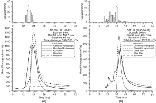
The value CE for the verification model is equal to or exceeds 0.70, excluding that for four events (Typhoon Bess on 22 September 1971, Typhoon Dinah on 20 September 1977, a storm on 6 March 2007 and a storm on 29 January 2008), and the error of peak discharge is less than 30% in all but six events. The error in the arrival time of the peak for all examined events is four hours or less, except for a storm on 6 March 2007. The comparison results indicate that the observations and simulations have an acceptable goodness-of-fit. Although the observations and simulations are not in full agreement, because of the complex behaviours of watershed responses, the calibration and verification results can still be applied to determine the usability of the proposed model. Furthermore, this model can also be applied in further applications.

Generation of runoff components

In this investigation of hydrological modelling, four hydrograph components are theoretically defined, and five runoff components must be identified for real runoff routings. These five components are surface runoff, rapid subsurface runoff, delayed subsurface runoff, groundwater runoff and baseflow. Surface runoff, rapid subsurface runoff, delayed subsurface runoff and groundwater runoff are generated by rainfall events, and are called “new discharges.” The baseflow is the groundwater flow before the rainfall starts, and is the lowest discharge of a rising limb in a total flow hydrograph when it is a constant. Therefore, baseflow can be called “old discharge” and is not a new flow generated by the present rainfall–runoff event.

In reality, various components of excessive streamflow from a typhoon event are difficult to correctly measure and divide. An alternative solution, which is the proposed model, was applied to generate hydrograph components. Horizontal outflows of the three serial linear reservoirs with one reservoir in parallel that simulate surface runoff, rapid and delayed subsurface runoff and groundwater runoff were obtained based on calibrated parameters determined from rainfall and streamflow data.

Table 5 lists the hydrograph characteristics of quick and slow components for 38 calibrated rainfall–runoff events. The amount of a slow flow is smaller than that of a quick runoff; and the ratios of slow flows to quick flows are 20.81–98.39%. From this comparison, this study infers that the amount of a slow runoff is always smaller than that of a quick runoff in a rainfall–runoff process. According to the simulation results (Table 5), the peak discharges for slow flows are smaller than those of quick flows (4.85–56.40%), and the amount of time taken to reach peak discharge for quick flows is shorter than that for slow flows (1–21 h). These simulation results correlate with our expectations. Throughout a rainfall–runoff event, the greatest proportion of streamflow originates from quick runoff, while the smaller portion consists of subsurface runoff, including rapid and delayed subsurface flows. Here, a slow flow is defined as the sum of subsurface and groundwater flows from a rainfall event.

Table 5  Hydrograph characteristics of quick and slow flows for 38 calibrated events

Event name (date)	Total discharge (m^3/s)		Peak discharge (m^3/s)		Time to peak (h)
	Quick	Slow	Quick	Slow	Quick	Slow
Typhoon Cora (1966-09-06)	4967.00	3476.19	778.85	143.67	22	24
Typhoon Betty (1972-08-16)	7679.83	4409.19	510.57	166.85	32	34
Typhoon Billie (1976-08-09)	1892.99	948.16	212.38	23.20	21	25
Typhoon Vera (1977-07-31)	5841.19	4243.69	846.28	145.87	24	28
Typhoon Ora (1978-10-12)	22639.24	10752.75	1332.63	234.92	36	57
Typhoon Irving (1979-08-14)	10150.04	5946.84	906.48	259.70	41	43
Storm (1980-11-19)	5228.03	3019.03	734.81	125.55	32	35
Typhoon Andy (1982-07-29)	2998.59	2319.19	340.08	67.41	19	26
Typhoon Cecil (1982-08-09)	7698.94	5327.74	607.13	146.30	14	33
Storm (1983-10-12)	5741.39	2957.28	637.98	72.86	20	24
Storm (1983-10-14)	5643.00	2458.92	792.65	100.49	21	25
Storm (1984-06-02)	7144.74	3390.66	900.10	96.31	35	40
Storm (1984-11-18)	5090.46	4739.72	349.74	98.55	35	49
Typhoon Nelson (1985-08-22)	8270.42	4896.83	1108.37	107.70	24	31
Typhoon Alex (1987-07-27)	3073.47	2188.87	431.39	61.83	14	18
Typhoon Abe (1990-08-30)	8411.87	4298.66	629.31	226.88	22	23
Storm (1990-09-01)	2743.92	570.94	267.96	13.00	15	28
Storm (1990-09-02)	5782.34	4342.34	573.77	124.67	27	31
Storm (1994-06-18)	3118.74	2498.25	340.61	99.47	19	24
Typhoon Fred (1994-08-20)	2345.81	1854.17	245.82	39.59	41	44
Typhoon Gladys (1994-09-01)	3058.76	2538.33	324.55	36.15	19	25
Typhoon Herb (1996-07-31)	7715.03	7285.35	938.14	215.42	28	30
Typhoon Winnie (1997-08-17)	8752.92	8612.32	649.92	366.58	38	39
Typhoon Amber (1997-08-29)	8210.89	6657.44	908.55	280.54	21	24
Storm (1999-09-26)	880.85	527.15	59.25	7.41	31	35
Typhoon Bebinca (2000-11-08)	8855.66	5100.50	551.26	110.98	30	39
Typhoon Rananim (2004-08-12)	610.99	527.10	79.95	12.59	15	19
Storm (2004-08-17)	270.20	219.57	21.40	4.08	17	20
Storm (2004-10-01)	748.66	421.16	59.98	11.67	30	33
Storm (2005-05-09)	3776.27	3198.41	237.07	80.70	39	41
Storm (2005-09-10)	923.61	598.47	77.30	12.51	37	40
Storm (2005-12-04)	709.38	376.39	37.04	6.75	14	17
Storm (2005-12-11)	3511.39	1500.79	132.58	44.31	29	33
Storm (2006-06-06)	1444.28	881.20	94.70	21.34	39	41
Storm (2007-06-15)	2120.74	1112.79	178.45	22.84	21	25
Storm (2007-09-04)	2498.97	1807.38	229.56	35.55	45	49
Storm (2008-05-30)	2403.50	2023.79	168.30	33.42	14	32
Storm (2008-10-10)	3655.98	2299.35	320.15	179.05	12	13

Times to peak for runoff components

Clarifying the times to peak for runoff components is vital for determining the time required to produce the maximum discharge of a runoff hydrograph. This study first addresses the time to peak characteristic. The time to peak for a quick runoff is less than that of a slow runoff (Table 5). The relationships between the peak time of rainfall and the time to peak of runoff components is plotted in Fig. 7. As these relationships are not simple linear correlations, the original values are translated into natural logarithm forms (or power forms) and linear regression is applied for fitting.

Fig. 7 Relationships of peak times between simulated hydrograph components and rainfall observation.

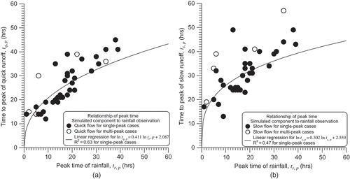
Figure 7(a) and (b) shows the correlations between peak times of hyetographs and times to peak for hydrograph components, quick runoff and slow runoff. These power correlations (Fig. 7) exclude multi-peak rainfall–runoff events. The power relationship for peak time between rainfall and quick runoff (R² = 0.63) is more distinct than that for between rainfall and slow runoff (R² = 0.47). The established relationship between rainfall and quick runoff is significantly correlated compared to that between rainfall and slow runoff. This is because slow water flowing beneath the land surface is influenced not only by infiltration resulting from rainfall, but also by porosity, soil moisture and the hydraulic conductivity of soil layers. The results of the analysis demonstrate that the time to peak of a quick flow is significantly correlated with the peak time of a hyetograph, and slow flow is visually correlated with rainfall.

Based on these results, we conclude that the time to peak of a slow runoff is higher than that of a quick runoff. Moreover, the times to peak of both hydrograph components are related to the time of peak rainfall, and their relationships are power forms excluding multi-peak events.

Peak discharges of runoff components

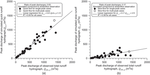
Identifying the characteristic of peak discharge of a hydrograph is essential when designing hydraulic structures. Hence, this study also analyses the relationships between hydrograph components and observed total runoffs in terms of peak discharges. The peak discharge of a quick runoff typically exceeds that of a slow runoff (Table 5). The analytical findings indicate that a large total runoff hydrograph (sum of quick runoff, slow runoff, and baseflow) has a large peak for a quick runoff and is larger than that of a slow runoff.

The relationships for peak discharges between component hydrographs and observations of total runoff are plotted in Fig. 8, with the formula results for both linear regression results. According to R² values (i.e. R² = 0.93 and R² = 0.58), two linear relationships exist between the simulated quick and slow runoffs to total runoff observations. The correlation between quick runoff and total runoff is more significant than that between slow runoff and total runoff, as slow runoff in an aquifer is more complex than surface runoff (quick runoff) that flows on the ground surface. While the peak discharges of quick runoff are slightly smaller than those of observed total runoff, the peaks of slow runoff are significantly smaller than those of observed total runoff (Fig. 8). With respect to multi-peak and single-peak cases, the ratios are 1–0.83 for observed total runoffs to surface (quick) runoffs and 1–0.17 for observed total runoffs to slow runoffs. Based on the ratios of peak discharge between total runoff observations and both runoff components, the peak discharge of a quick runoff is 4.88 times that of a slow runoff.

Fig. 8 Relationships of peak discharges between simulated hydrograph components and observed total runoff.

Total discharges of runoff components

Finally, this study discusses the final characteristic of hydrograph components, total discharge (Table 5). The total discharge of a hydrograph is equivalent to the hydrograph volume, as hydrograph volume is a multiple of total discharge; and the multiple is 3600 s (1 hour) for the time interval between the observations conducted in Taiwan. Theoretically, the total discharge of a surface (quick) runoff should exceed that of a slow runoff during a rainfall–runoff episode. Table 5 summarizes the correlation results for all cases.

The comparison results of individual components and observed total runoff to further identify the ratio percentages of component flows during rainfall–runoff events are plotted in Fig. 9. For the same events, the points representing specific values for the total discharges of surface (quick) runoffs to those of total runoffs (Fig. 9(a)) exceed those resulting from the ratios of slow runoffs to total runoffs (Fig. 9(b)). The two figures illustrate the linear correlations. Similar to the analysis results of Fig. 8, linear regression is used to determine the relationships of total discharges between total runoff and both components, quick runoff and slow runoff.

Fig. 9 Relationships of total discharges between simulated hydrograph components and observed total runoff.

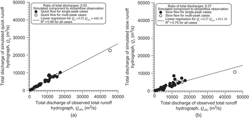
According to the analysis results of Fig. 9, the total discharge of quick flow is larger than that of slow flows in rainfall–runoff events. The variations, which are generally straight lines, can be found for percentages of quick flows to total flows (R² = 0.96) and slow flows to total flows (R² = 0.75). Regardless of whether rainfall–runoff events have a single peak or multiple peaks, the total discharge of a surface runoff is 52% that of total runoff and 27% that of a slow runoff; whereas the remainder is comprised of baseflow components. Based on the ratios for total discharge of total runoff to those of both runoff components, the total discharge of a quick runoff is 1.93 times that of a slow runoff.

Synthetic illustrations of outlet-runoff components

The structure of the proposed model can separate an outlet streamflow into several parts and then identify the runoff characteristics of each part. Generally, a quick (surface) runoff hydrograph has a large peak discharge, whereas a slow runoff hydrograph has a relatively smaller peak flow.

Excluding multi-peak rainfall–runoff events, the time to peak of hydrograph components is correlated with peak times of hyetographs; and both relationships of quick runoff to rainfall and slow runoff to rainfall are increasing power correlations. Furthermore, linear correlations of peak discharges increasingly occur between the flow components and the observed total flows for all cases, including multi-peak and single-peak storms. The strength of the linear correlation resulting from quick runoff is higher than that from slow runoff. The peak discharge of a quick runoff is approximately 83% of the total runoff peak and 17% of the peak flow for a slow flow. Moreover, the relationships for total discharges between hydrograph components and observations of total runoff are also increasingly linear correlations for all storms. A total quick/surface runoff discharge is 52% of the total runoff discharge and 27% for a slow runoff discharge.

Finally, the characteristics of quick and slow runoff hydrographs can be easily determined, as this study has identified the hydrograph characteristics of flow components, such as time to peak, peak discharge and total discharge. The analytical results facilitate the evaluations of hydrograph characteristics for quick and slow runoffs based on the given hyetographs and total runoff hydrographs. The evaluations of hydrograph components in a river-outlet provide a valuable reference for water resource management in Taiwan.

CONCLUSIONS

This study used a model of three serial reservoirs with one parallel reservoir, involving seven parameters to simulate the runoff components of a river outlet. These calibrated parameters were divided into four groups. The largest variation was the rate coefficient for surface runoff, followed by the antecedent value and rate coefficients for rapid subsurface runoff and infiltration, delayed subsurface runoff, percolation and groundwater runoff. As the complexity of the generation mechanism of natural flow increased, the range of its corresponding parameter increased, due to several unknown/uncontrolled causes.

Eight constraints of the model parameters make them conform to physical reality. These constraints can offer effective assistance when observing runoff components in the streamflows of a watershed outlet. The proposed model is suitable to evaluate the runoff components relating to rainfall–streamflow observations in this watershed and to fit data from basins in other parts of Taiwan. These evaluation results, which result from data in this and other watersheds, can be synthetically applied for watershed management in Taiwan. The structure of three serially-connected linear reservoirs with one in parallel simulate the various components of a watershed outlet hydrograph. The storage values at each reservoir are used to derive the different unit hydrographs. The expression of each unit hydrograph has an exponential function, derived from the convolution integral and continuity equation. The discharges of the runoff components resulting from specific opening sizes reflect the generation of surface runoff, subsurface runoff (rapid and delayed subsurface flows) and groundwater runoff, in which a surface runoff is a quick flow, while a slow flow is a sum of groundwater, and delayed and rapid subsurface runoff.

The quick and slow runoffs that were regenerated by using the proposed model revealed the characteristics of runoff components (that is, a quick/surface runoff acts as a sharp point in a period after rainfall and terminates within a short time, whereas slow flow stops after a long period). Therefore, the shape of a quick runoff hydrograph is more concentrated and shifts forward compared to that of a slow flow.

The following conclusions are made based on study results:

1.	The time to peak for both hydrograph components of single-peak events is an increasing power correlation corresponding to the peak time of a hyetograph. The relationship of quick runoff and rainfall is markedly stronger than that of slow runoff and rainfall.
2.	The peak discharges of hydrograph components for all events are directly and linearly proportional to the total runoff observations. The linear correlation between quick runoff and total runoff is higher than that between slow runoff and total runoff. The ratio of a quick runoff to the observed total runoff is approximately 83%, while it is 17% for slow flow for the same total runoff.
3.	The total volume of quick runoff component is 52% of total runoff and that of slow runoff is 27%. When rainfall conditions and the total runoff hydrographs are known, the results of this study significantly contribute to efforts to evaluate the hydrograph characteristics of quick and slow runoff and, thus, provide a valuable reference for watershed management in Taiwan.

Acknowledgements

The authors would like to thank the National Science Council of the Republic of China (NSC 100-2313-B-434-001) for financially supporting this research.

REFERENCES

- Agirre , U. 2005 . Application of a unit hydrograph based on subwatershed division and comparison with Nash's instantaneous unit hydrograph . Catena , 64 : 321 – 332 .
- Ahmad , M.M. , Ghumman , A.R. and Ahmad , S. 2009 . Estimation of Clark's instantaneous unit hydrograph parameters and development of direct surface runoff hydrograph . Water Resources Management , 23 : 2417 – 2435 .
- Andréassian , V. 2001 . Impact of imperfect rainfall knowledge on the efficiency and the parameters of watershed models . Journal of Hydrology , 125 : 206 – 223 .
- Bastin , G. 1984 . Optimal estimation of the average rainfall and optimal selection of raingauge locations . Water Resources Research , 20 : 463 – 470 .
- Bhadra , A. 2010 . rainfall–runoff modeling: comparison of two approaches with different data requirements . Water Resources Management , 24 : 37 – 62 .
- Carcano , E.C. 2008 . Jordan recurrent neural network versus IHACRES in modelling daily streamflows . Journal of Hydrology , 362 : 291 – 307 .
- Chen , R.S. , Pi , L.C. and Huang , Y.H. 2003 . Analysis of rainfall–runoff relation in paddy fields by diffusive tank model . Hydrological Processes , 17 : 2541 – 2553 .
- Cheng , K.S. , Lin , Y.C. and Liou , J.J. 2008a . Rain-gauge network evaluation and augmentation using geostatistics . Hydrological Processes , 22 : 2554 – 2564 .
- Cheng , S.J. 2011 . Raingauge significance evaluation based on mean hyetographs . Natural Hazards , 56 : 767 – 784 .
- Cheng , S.J. , Hsieh , H.H. and Wang , Y.M. 2007 . Geostatistical interpolation of space–time rainfall on Tamshui River Basin, Taiwan . Hydrological Processes , 21 : 3136 – 3145 .
- Cheng , S.J. 2008b . The storage potential of different surface coverings for various scale storms on Wu-Tu watershed, Taiwan . Natural Hazards , 44 : 129 – 146 .
- Cheng , S.J. , Lee , C.F. and Lee , J.H. 2010 . Effects of Urbanization Factors on Model Parameters . Water Resources Management , 24 : 775 – 794 .
- Cheng , S.J. and Wang , R.Y. 2002 . An approach for evaluating the hydrological effects of urbanization and its application . Hydrological Processes , 16 : 1403 – 1418 .
- Clarke , R.T. 1973 . A review of some mathematical models used in hydrology, with observations on their calibration and use . Journal of Hydrology , 19 : 1 – 20 .
- Croke , B.F.W. , Letcher , R.A. and Jakeman , A.J. 2006 . Development of a distributed flow model for underpinning assessment of water allocation options in the Namoi River Basin, Australia . Journal of Hydrology , 319 : 51 – 71 .
- Duan , Q. , Gupta , V.K. and Sorooshian , S. 1993 . Shuffled complex evolution approach for effective and efficient global minimization . Journal of Optimization Theory Application , 76 : 501 – 521 .
- Evans , J.P. 2003 . Improving the characteristics of streamflow modeled by regional climate models . Journal of Hydrology , 284 : 211 – 227 .
- Franchini , M. and O'Connell , P.E. 1996 . An analysis of the dynamic component of the geomorphologic instantaneous unit hydrograph . Journal of Hydrology , 175 : 407 – 428 .
- Goovaerts , P. 2000 . Geostatistical approaches for incorporating elevation into the spatial interpolation of rainfall . Journal of Hydrology , 228 : 113 – 129 .
- Hashino , M. , Yao , H. and Yoshida , H. 2002 . Studies and evaluations on interception processes during rainfall based on a tank model . Journal of Hydrology , 255 : 1 – 11 .
- Hsieh , L.S. and Wang , R.Y. 1999 . A semi-distributed parallel-type linear reservoir rainfall–runoff model and its application in Taiwan . Hydrological Processes , 13 : 1247 – 1268 .
- Huang , H.J. 2008a . Effect of growing watershed imperviousness on hydrograph parameters and peak discharge . Hydrological Processes , 22 : 2075 – 2085 .
- Huang , S.Y. 2008b . Identifying peak-imperviousness–recurrence relationships on a growing-impervious watershed, Taiwan . Journal of Hydrology , 362 : 320 – 336 .
- Jakeman , A.J. and Hornberger , G.M. 1993 . How much complexity is warranted in a rainfall–runoff model? . Water Resources Research , 29 : 2637 – 2649 .
- Jakeman , A.J. , Littlewood , I.G. and Whitehead , P.G. 1990 . Computation of the instantaneous unit hydrograph and identifiable component flows with application to two upland catchments . Journal of Hydrology , 117 : 275 – 300 .
- Jin , C.X. 1992 . A deterministic gamma-type geomorphologic instantaneous unit hydrograph based on path types . Water Resources Research , 28 : 479 – 486 .
- Kliment , Z. and Matoušková , M. 2009 . Runoff changes in the Šumava Mountains (Black Forest) and the foothill regions: extent of influence by human impact and climate change . Water Resources Management , 23 : 1813 – 1834 .
- Lebel , T. and Bastin , G. 1985 . Variogram identification by the mean squared interpolation error method with application to hydrologic field . Journal of Hydrology , 77 : 31 – 56 .
- Lee , Y.H. and Singh , V.P. 2005 . Tank model for sediment yield . Water Resources Management , 19 : 349 – 362 .
- Madsen , H. 2000 . Automatic calibration of a conceptual rainfall–runoff model using multiple objectives . Journal of Hydrology , 235 : 276 – 288 .
- Mays , L.W. and Taur , C.K. 1982 . Unit hydrographs via nonlinear programming . Water Resources Research , 18 : 744 – 752 .
- Melone , F. , Corradini , C. and Singh , V.P. 1998 . Simulation of the direct runoff hydrograph at basin outlet . Hydrological Processes , 12 : 769 – 779 .
- Moramarco , T. , Melone , F. and Singh , V.P. 2005 . Assessment of flooding in urbanized ungauged basins: a case study in the upper Tiber area, Italy . Hydrological Processes , 19 : 1909 – 1924 .
- Nash, J.E., 1957. The form of the instantaneous unit hydrograph. In: Surface water, prevision, evaporation (General Assembly of Toronto 3–14 September 1957). Wallingford, UK: IAHS Press, IAHS Publ. 45, 112–121. http://iahs.info/redbooks/a045/045011.pdf (http://iahs.info/redbooks/a045/045011.pdf)
- Nash , J.E. and Sutcliffe , J.V. 1970 . River flow forecasting through conceptual models: 1. a discussion of principles . Journal of Hydrology , 10 : 282 – 290 .
- Nayak , P.C. , Sudheer , K.P. and Ramasastri , K.S. 2005 . Fuzzy computing based rainfall–runoff model for real time flood forecasting . Hydrological Processes , 19 : 955 – 968 .
- Nourani , V. , Singh , V.P. and Delafrouz , H. 2009 . Three geomorphological rainfall–runoff models based on the linear reservoir concept . Catena , 76 : 206 – 214 .
- O'Connell , P.E. and Todini , E. 1996 . Modelling of rainfall, flow and mass transport in hydrological systems: an overview . Journal of Hydrology , 175 : 3 – 16 .
- Schreider , S. 2002 . Detecting changes in streamflow response to changes in non-climatic catchment conditions: farm dam development in the Murray-Darling basin, Australia . Journal of Hydrology , 262 : 84 – 98 .
- Sugawara , M . 1979 . Automatic calibration of the tank model . Hydrological Sciences Bulletin , 24 : 375 – 388 .
- Sugawara , M. 1995 . “ Tank model ” . In Computer models of watershed hydrology , Edited by: Singh , V.P. Littleton , CO : Water Resources Publications .
- Syed , K.H. 2003 . Spatial characteristics of thunderstorm rainfall fields and their relation to runoff . Journal of Hydrology , 271 : 1 – 21 .
- Yue , S. and Hashino , M. 2000 . Unit hydrographs to model quick and slow runoff components of streamflow . Journal of Hydrology , 227 : 195 – 206 .