Daily streamflow forecasting using a wavelet transform and artificial neural network hybrid models

Abstract

New wavelet and artificial neural network (WA) hybrid models are proposed for daily streamflow forecasting at 1, 3, 5 and 7 days ahead, based on the low-frequency components of the original signal (approximations). The results show that the proposed hybrid models give significantly better results than the classical artificial neural network (ANN) model for all tested situations. For short-term (1-day ahead) forecasts, information on higher-frequency signal components was essential to ensure good model performance. However, for forecasting more days ahead, lower-frequency components are needed as input to the proposed hybrid models. The WA models also proved to be effective for eliminating the lags often seen in daily streamflow forecasts obtained by classical ANN models. 

Editor D. Koutsoyiannis; Associate editor L. See

Citation Santos, C.A.G. and Silva, G.B.L., 2013. Daily streamflow forecasting using a wavelet transform and artificial neural network hybrid models. Hydrological Sciences Journal, 59 (2), 312–324.

Résumé

Nous proposons de nouveaux modèles hybrides d’ondelettes et de réseaux de neurones artificiels (WA) pour la prévision des débits journaliers aux horizons de 1, 3, 5 et 7 jours, basés sur les composantes basse fréquence du signal d’origine (approximations). Les résultats montrent que les modèles hybrides proposés donnent des résultats significativement meilleurs que les réseaux de neurones artificiels classiques (ANN) pour toutes les situations étudiées. Pour les prévisions à court terme (1 jour), des informations sur les composantes haute fréquence du signal sont essentielles pour assurer une bonne performance du modèle. Pour la prévision à plus long terme, les composants basse fréquence sont nécessaires comme entrée des modèles hybrides proposés. Les modèles WA se sont également avérés efficaces pour éliminer le délai souvent observé dans les prévisions de débits journaliers obtenus par des modèles ANN classiques.

Key words:

• discharge prediction
• time series
• signal decomposition

Mots clefs:

• prévision de débit
• série chronologique
• décomposition du signal

INTRODUCTION

Streamflow forecasting is essential in many activities involving the operation and optimization of water resources. For this reason, the development of mathematical models able to provide more reliable long-term forecasting has attracted the attention of hydrologists through time.

In the last decade, the applications of artificial neural networks (ANNs) to various aspects of hydrological modelling has been the objective of several investigations (ASCE Task Committee 2000a, 2000b, Maier and Dandy 2000, Cigizoglu 2004, Rajurkar et al. 2004, Bowden et al. 2005, Chandramouli et al. 2007, Coulibaly and Evora 2007, Elshorbagy and Parasuraman 2008, Feng et al. 2008, Singh et al. 2009). The interest has been motivated by the complex nature of hydrological systems and the capacity of ANNs to represent highly nonlinear correlations, as well as the fast and flexible modelling process, with no need for the complex nature of the underlying processes considered to be explicitly described in mathematical terms.

In the streamflow forecasting field, in particular, several works have demonstrated the good performance of ANN models (Dawson and Wilby 1999, ASCE Task Committee 2000b, Jayawardena and Fernando 2001, Birikundavyi et al. 2002, Shrestha et al. 2005, Dawson et al. 2006, Kerh and Lee 2006, Kisi 2007, 2008, Pulido-Calvo and Portela 2007, Kentel 2009, Santos et al. 2009, Sarmiento and Neira 2009, Turan and Yurdusev 2009, Besaw et al. 2010, Farias et al. 2011, He et al. 2011, Santos and Morais 2013). Because they overcome several difficulties related to traditional models, such as autoregressive integrated moving average models (ARIMA) and other linear and nonlinear models, ANN models have been established as one of the main hydrological forecasting tools and have been embraced enthusiastically by practitioners in water resources.

However, some difficulties are still present in the application of ANNs to streamflow forecasting. Wu et al. (2009) comment that noise generally present in streamflow series may influence the prediction quality and mention that cleaner signals used as model inputs will improve the ANN model performance. Wu et al. (2009) also note that, in daily flow modelling, the strong correlation present in the data tends to introduce lagged predictions in ANN models. The issue of lagged predictions in the ANN model has been mentioned by other researchers (e.g. Dawson and Wilby 1999, Jain and Srinivasulu 2004, de Vos and Rientjes 2005, Muttil and Chau 2006). Moreover, Cannas et al. (2006) mention that ANNs and other methods frequently have limitations with non-stationary data.

In order to deal with these issues, the application of methods to pre-process input data has been highlighted as an efficient alternative to improve the performance of ANN models. An example of such a method is wavelet analysis, which has recently received much attention. Wavelet analysis provides useful decomposition of original time series into high- and low-frequency components, so that wavelet-transformed data can improve the ability of a forecasting model by capturing useful information at various resolution levels (Kim and Valdés 2003).

The number of works involving the application of hybrid wavelet and ANN (WA) models in the context of streamflow forecasting has significantly increased in recent years. Anctil and Tape (2004) compare the 1-day ahead streamflow forecasting performance of multiple-layer artificial neurons and a neuro-wavelet hybrid system at two sites. Cannas et al. (2006) developed a hybrid model for monthly rainfall–runoff forecasting in Italy. Adamowski (2007, 2008a, 2008b) developed a completely new method of wavelet and cross-wavelet-based forecasting of floods. Wang et al. (2009) developed a wavelet neural network model to forecast the inflow at the Three Gorges Dam on the Yangtze River. Partal (2009) employed a wavelet neural network structure for the forecasting of monthly river flows in Turkey and compared the performance of WA methods with the conventional ANN methods. Kisi (2008, 2009) explored the use of WA models for daily flow forecasting of intermittent rivers. Wu et al. (2009) coupled three data pre-processing techniques: moving average (MA), singular spectrum analysis (SSA) and wavelet multi-resolution analysis (WMRA), with an ANN to improve the estimate of daily flows. Adamowski and Sun (2010) proposed a method based on coupling discrete wavelet transforms and ANNs for flow forecasting at lead times of 1 and 3 days in non-perennial rivers in semi-arid watersheds. All these studies found that the WA models outperformed the other models (such as multiple linear regression and regular ANNs that were studied for hydrological forecasting applications.

Even with the increasing number of investigations about this issue, specific studies involving the assessment of WA model performance in the forecasting of daily streamflow for more than 3 days ahead is still very limited and restricted to a few regions in the world. For this reason, it is believed that new investigations on the issue may contribute to extend and complement the results and conclusions already obtained in other research. In this sense, this work has the main objectives of assessing the efficiency of WA models in the forecasting of daily streamflows for 1, 3, 5 and 7 days ahead and comparing the results with models based on regular ANNs. The majority of the applications involving WA models published until now used the high-frequency components (details) extracted from the wavelet analysis as the main input variable. A particularity of the present work is the use of only low-frequency sub-series (approximations) as model input.

This research was mainly motivated by the fact that 90% of the electric power produced in Brazil is generated by hydroelectric systems. For this reason, the availability of good forecasting of streamflow to reservoirs is essential to the proper mid- and long-term generation planning and to the optimization of short-term generation planning. Nowadays, the National Electrical System Operator (ONS – Operador Nacional do Sistema Elétrico) uses stochastic models for streamflow forecasting, but they have limited accuracy (Guilhon et al. 2007). Therefore, there is the need to test, develop and improve other forecasting methodologies to contribute to the improvement of the planning process and operation programming of the National Interlinked System (SIN – Sistema Interligado Nacional).

MATERIALS AND METHODS

Wavelet transform

Mathematical transforms are applied to signals to obtain more information about them, when they are not available in their raw form. There are many transforms to be applied, among which Fourier transforms are the most popular. Aiming at keeping the localization of frequency over time in a signal analysis, a possibility would be to make a windowed Fourier transform (WFT), using a certain window size and sliding it over time, calculating the fast Fourier transform (FFT) at each time and using only the data inside the window. This would solve the problem of frequency localization, but it would still depend on the window size used.

The main problem with WFT is the inconsistent treatment of different frequencies; that is, in low frequencies there are so few oscillations inside the window that the frequency localization is lost, while in high frequencies there are so many oscillations that the time localization is lost. Besides, WFT also supposes that the signal may be decomposed into sinusoidal components.

The wavelet analysis focuses on solving these problems of decomposing or transforming a uni-dimensional time series into a fuzzy bi-dimensional image simultaneously in a time–frequency domain. Then, it is possible to obtain information about the amplitude of any periodic signal within the series and how this amplitude varies with time. The wavelet analysis may be used in the continuous or the discrete form. For the present study, the discrete wavelet transform is sufficient and suitable for the application proposed.

Discrete wavelet transform

A discrete wavelet transform is obtained from a continuous representation by discretizing dilation and translation parameters such that the resulting set of wavelets constitutes a frame. The dilation parameters are typically discretized by an exponential sampling with a fixed dilation step, and the translation parameter by integer multiples of a dilation-dependent step (Daubechies 1992). Unfortunately, the resulting transform is a variant under translations, a property which makes it less attractive for the analysis of non-stationary signals.

Calculating wavelet coefficients at every possible scale requires a fair amount of work and generates a lot of data, but it would be possible to calculate only a subset of scales and positions. It turns out, rather remarkably, that if we choose scales and positions based on powers of two (so-called dyadic scales and positions), then the analysis will be much more efficient and just as accurate. Such an analysis is obtained from the discrete wavelet transform (DWT). An efficient way to implement this scheme using filters was developed by Mallat (1989). The Mallat algorithm is, in fact, a classical scheme known in the signal processing community as a two-channel sub-band coder. This very practical filtering algorithm yields a fast wavelet transform, i.e. a box into which a signal passes, and out of which wavelet coefficients quickly emerge.

One-stage filtering: approximations and details

The wavelet transform can be defined as a tree of low- and high-pass filters. The low-pass filters reduce the amount of information in the raw signal, Q_o (observed streamflow, in the present case), and the high-pass filters represent the information that is lost (Fig. 1(a)).

Fig. 1 Examples of (a) simple filtering process and (b) filtering process with downsampling decomposition.

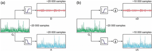
For many cases, the low-frequency content of the signal is the most important part. It is what gives the signal its identity, and that is the reason why the low-frequency content was chosen in the present study as input to the proposed hybrid WA models. The high-frequency content, on the other hand, imparts flavour or nuance. In wavelet analysis, low-frequency content is referred to as “approximations” and high-frequency content as “details”. The approximations are the high-scale, low-frequency components of the signal, and the details are the low-scale, high-frequency components.

The filtering process, at its most basic level, is shown in Fig. 1(a). The original signal, Q_o, passes through two complementary filters (high- and low-pass) and emerges as two signals. Unfortunately, when this operation is performed, there will be twice as much data as when the process started. Suppose, for instance, that the original signal Q_o consists of 20 000 samples of observed daily runoff data. Then the resulting signals will each have 20 000 samples, giving a total of 40 000 (Fig. 1(a)). The signals A and D are interesting, but there are 40 000 values instead of the original 20 000. There is a more suitable way to perform the decomposition using wavelets. For example, it is possible to keep only one point out of two in each of the two 20 000-length samples to get the complete information. This is the notion of downsampling. Then, two sequences called cA and cD are produced (Fig. 1(b)), and this process with downsampling produces DWT coefficients (c).

The actual lengths of the detail and approximation coefficient vectors are slightly more than half the length of the original signal. This has to do with the filtering process, which is implemented by convolving the signal with a filter. This is defined as one-stage discrete wavelet transform of signal Q_o.

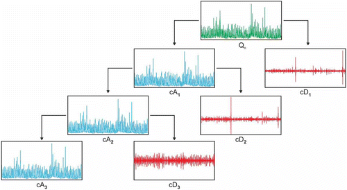
Multiple-level decomposition

The decomposition process can be iterated, with successive approximations being decomposed in turn, so that the original signal is broken down into many lower-resolution components. This is referred to as the wavelet decomposition tree (Fig. 2). Since the analysis process is iterative, in theory it can be continued indefinitely. In reality, the decomposition can proceed only until the individual details consist of a single sample or pixel. In practice, a suitable number of levels, based on the nature of the signal, or on a suitable criterion such as entropy, should be selected. The approximation (A) and detail (D) components can be obtained by a reconstruction procedure. It is also important to observe that Q_o = A₁ + D₁, or that A₁ = A₂ + D₂, and in the same way Q_o = A₃ + D₃ + D₂ + D₁.

Fig. 2 Decomposition tree at three levels.

Mother wavelet

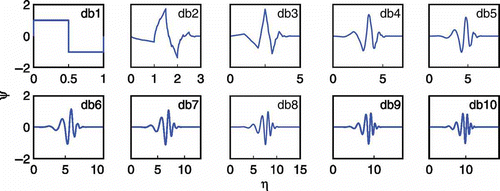
There are many basic wavelets that can be used in this type of transformation. The present application will use Daubechies wavelets, since they have been used in several applications (e.g. Cannas et al. 2006, Kisi 2008, 2009). They are named after Ingrid Daubechies and are a family of orthogonal wavelets defining a discrete wavelet transform and characterized by a maximal number of vanishing moments for some given support. With each wavelet type of this class, there is a scaling function (also called a father wavelet) which generates an orthogonal multi-resolution analysis. In Fig. 3, Daubechies wavelets may be seen from order 1 up to 10 (note, db1 is similar to the Haar wavelet). These wavelets have no explicit expression, except for db1, Haar wavelet. Most of the dbN are not symmetric, and for some, the asymmetry is well pronounced. Regularity increases with order. The N index in dbN indicates the order, which in theory may vary from 1 to infinity.

Fig. 3 Daubechies wavelets (from order 1 to 10).

Artificial neural network

Artificial neural networks are computational tools inspired by the functioning of the human brain and nervous system. The great capacity of the biological neural system to perform complex tasks has been attributed to the parallel and distributed processing nature of the biological neurons. The ANN imitates such structures where the calculus is processed through simple unities, called artificial neurons, which are interconnected to form a network.

Due to the great quantity of information available in the literature about ANNs (ASCE Task Committee 2000a, 2000b, Haykin 2005), the description presented here is short and limited to the needs of this study. In this work, the ANN used was the multilayer perceptron (MLP). The typical structure of this ANN is shown in Fig. 4.

Fig. 4 MLP network with one intermediate (hidden) layer.

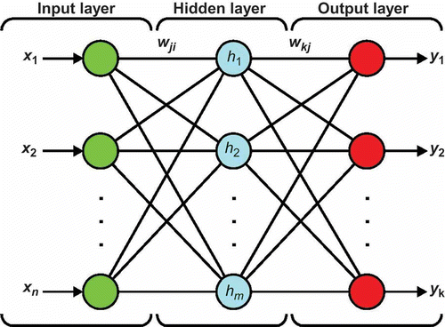
The data (x₁, x₂, …, x_n) are introduced in the input layer and the network progressively processes such data through subsequent layers, producing a result (y₁, y₂, …, y_k) in the output layer. The input neurons are linked to those in the intermediate layer through w_ji weights and the neurons in the intermediate layer are linked to those in the output layer through w_ki weights (see below). The network maps out the relationship between the input data and the output variables based on the nonlinear activation functions.

Between the input and the output layers, multiple intermediate layers may be included. In theory, the increase in the number of intermediate layers improves the mapping capacity of the network. However, it also significantly increases the processing time and the necessity of memory for storage due to the great quantity of weights. Research has demonstrated that the use of a single intermediate layer is sufficient for an ANN to approximate any complex nonlinear function, and MLP with three layers has been proven to be enough to forecast and simulate several problems related to water resources. For this reason, the setting given in Fig. 4 was used. The explicit correlation for the output values is given by:

(1)

where w_ji is the weight connecting the ith neuron in the input layer and the jth neuron in the hidden layer, w_kj is the weight connecting the kth neuron in the output layer and the jth neuron in the hidden layer, b_j is the bias for the jth hidden neuron, b_k is the bias for the kth output neuron, f_h is the activation function of the nodes in the hidden layer and f_o is the activation function of the nodes in the output layer.

Activation functions

Continuous and differential functions are necessary for relating inputs and outputs of ANNs. According to Haykin (2005), the sigmoid function is a good activation function due to its generally accepted behaviour. The tan-sigmoid function was chosen as the activation function for the hidden neurons (f_h). For the output layer neuron, a linear activation function (f_o) was used.

Training process

The determination of the ANN weights is made through a procedure called training, in which several input–output examples are presented to the ANN and its weights are iteratively modified until ANN reaches an acceptable mapping capacity, which is defined by the user. The training is performed by a back-propagation algorithm which has also been successfully applied to water resources systems.

In this approach, the Levenberg-Marquardt (LM) algorithm was used for the back-propagation training. The LM algorithm is a modification of the classic Newton algorithm for finding an optimum solution to a minimization problem (Daliakopoulos et al. 2005); it is designed to approach second-order training speed and accuracy without having to compute the Hessian matrix. Second-order nonlinear optimization techniques are usually faster and more reliable. Nowadays, the LM algorithm is, admittedly, the fastest for training an ANN of moderate size, in spite of requiring a superior amount of memory compared to other algorithms.

Performance evaluation

The efficiency of the models may be assessed using several statistical parameters that describe the degree of similarity among the data observed and those predicted by the model (Abrahart et al. 2007, Dawson et al. 2007, Napolitano et al. 2011). In this work, three indices were used, root mean square error (RMSE), mean absolute relative error (MARE) and coefficient of efficiency (CE):

(2)

(3)

(4)

where y_i corresponds to the observed values, corresponds to the values produced by the network, is the mean of the observed values and n is the sample size. The RMSE represents the variance of the error regardless of the size of the sample analysed. The best models are those which showed low RMSE and MARE and CE values close to 1.

Field data

The data used in this work correspond to the re-naturalized daily streamflow time series at the Sobradinho hydroelectric plant, in the São Francisco River, Brazil (Fig. 5). The hydroelectric plant, besides having the function of generating electric power (1 050 000 kW installed), is the main way of regulating the water resources in the region. It has a drainage basin of 498 968 km².

Fig. 5 Location of Sobradinho Dam and reservoir within the São Francisco River basin.

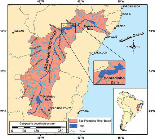
The data were extracted from the website of the National System Operator (ONS; Operador Nacional do Sistema, http://www.ons.org.br), the institution responsible for the operation of the interlinked electric system in Brazil. The data series has 18 900 points, referring to the period between 1 January 1931 and 29 September 1982, and the flows registered in the period are very high, with a maximum value of 18 525 m³/s and minimum of 602 m³/s. The main statistics of these data are given in Table 1. The flood period occurs from October to April, with maximum flood levels in March, at the end of the rainy season.

Table 1 Descriptive statistics for the observed daily streamflow into Sobradinho Dam (1931–1982).

Statistic	Value	Units
Arithmetic mean	2 811	m^3/s
Mode	1 381	m^3/s
Median	1 992	m^3/s
Harmonic mean	1 802	m^3/s
Geometric mean	2 217	m^3/s
Range	17 923	m^3/s
First quartile	1 267	m^3/s
Third quartile	3 960	m^3/s
Interquartile range	2 693	m^3/s
Median absolute deviation	1 643	m^3/s
Variance	4 374 353	(m^3/s)^2
Standard deviation	2 091	m^3/s
Coefficient of variation	0.74	—
Skewness	1.71	—
Kurtosis	4.61	—
Excess kurtosis	1.61	—

MODEL IMPLEMENTATION

ANN models

In this study, four ANN models ANN₁, ANN₃, ANN₅ and ANN₇ were built to forecast streamflows 1, 3, 5 and 7 days ahead, respectively. The models were built to forecast the flows from previously observed values. Thus, the output layer had only one neuron, corresponding to the flow forecast T days ahead (Q_t+T), and the input was formed by the flows observed on the current day and on the previous days (Q_t, Q_t–1, Q_t–2,…).

When an ANN is developed, the initial objective consists of finding an optimal architecture that permits the capture of the relationship between the input and output variables. There is no general rule that indicates the number of neurons to be used in the input and hidden layers. Normally, these quantities are defined by means of a trial-and-error procedure. In this work, for each of the four models, many settings were tested, considering as input flows from the previous 1 to 15 days. For each case, the number of neurons in the hidden layer was increased from 3 to 30, with an increment of three unities, until the RMSE of the training set was not found to improve significantly. The architectures that produced the best result in terms of RMSE for each model were chosen.

Hybrid wavelet–ANN models

The wavelet–ANN (WA) models are ANN models that use as input data sub-series obtained by means of a multi-resolution analysis. This analysis applies the wavelet transform to successively decompose the original signal into different resolution levels (scale), as explained earlier, producing low-frequency contents, the approximations (A), and high-frequency contents, the details (D). A schematic diagram of the proposed hybrid WA model is presented in Fig. 6.

Fig. 6 General structure of the proposed wavelet–ANN model.

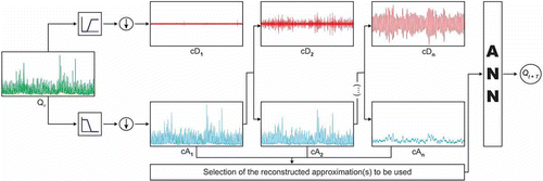
Decomposition process

The procedure of the multi-resolution analysis is presented in Fig. 2. Initially, the wavelet transform is applied to the original series (Q_o), considering the lowest possible scale. As a result of this first resolution level, the cD₁ component of the signal and the approximation cA₁ are obtained. The scale is doubled, and the wavelet transform is applied to the sub-series cA₁, the detail cD₂ and the approximation cA₂ being obtained. The process is applied iteratively to the next approximations, resulting in new levels of detail and approximation. In this way, the output decomposition structure contains the wavelet decomposition vector C and the book-keeping vector L, which are used to reconstruct the A and D components of the signal.

Once a signal has been decomposed this way, we can analyse the behaviour of the approximation information across the different scales. Furthermore, noise has a specific behaviour across scales and, hence, in many cases, we can separate the signal from the noise.

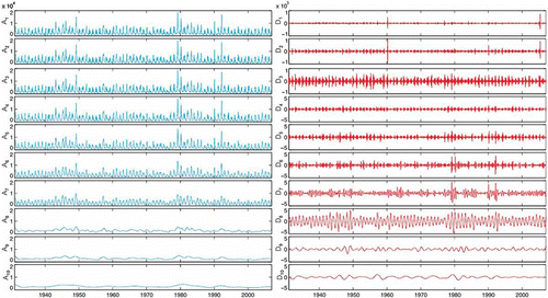
Among the Daubechies wavelets, the db10 was chosen for use in the decomposition of the flow signal due to its more detailed format, which permits better representation of the study series. Based either on the nature of the signal (a time series with 28 125 daily streamflow records) or on a suitable criterion such as entropy (the use of db10), a suitable number of 10 levels was selected, which resulted in 10 approximations and 10 details. Figure 7 shows the reconstructed approximations and details for the 10 levels of decomposition.

Fig. 7 Reconstructed approximations (A) and details (D) for 10 levels of decomposition.

Forecasting

In the same way as the regular ANN models, the WA models tested here were constructed to forecast the flows 1, 3, 5 and 7 days ahead: WA₁, WA₃, WA₅ and WA₇, respectively. The selection of appropriate components may have a positive effect on the ANN modelling capacity. In this work, the effectively used components were identified by a trial-and-error process, as well as based on the level of information that each component presents in relationship to the original Q_o signal.

In this case, several input options were tested, considering different sub-series of approximations and details, isolated (e.g. A₁) or combined (e.g. A₃ and A₄). For each situation, the performance of the corresponding model was assessed. Approximately 40 alternatives were initially considered.

The tests revealed that the use of the first five approximations (A₁, A₂, A₃, A₄ and A₅) produced the best results, because the approximations at higher levels (i.e. A₆, A₇, A₈, A₉ and A₁₀) lost significant information of the original signal. For example, the difference between the original signal Q_o (which is the same as A₁ + D₁) and the approximation A₁₀ is very apparent, and with a close look, it is possible to observe that the approximation A₆ has already lost important information (D₆). However, the incorporation of detail sub-series (D) in the input data did not directly result in significant improvement in the performance of the models. Based on this, only the first five approximations mentioned were selected as potential candidates to be the input variables of the hybrid system proposed.

It was also observed that, for forecasting with more days ahead (5 and 7 days), the use of more than one approximation improved the accuracy of the results. In these cases, new sub-series were built by means of the summation of individual approximations. This was found to decrease the number of inputs and, consequently, the ANN dimension, with no loss of important information for the modelling process. These new series were used as inputs for the WA model. The best input variables from among all the tested models ({A₁}; {A₁ + A₂}; {A₁ + A₂ + A₃}; {A₁ + A₂ + A₃ + A₄}; {A₁ + A₂ + A₃ + A₄ + A₅}; {A₂}; {A₂ + A₃}; {A₂ + A₃ + A₄}; …; {A₅}) are presented in Table 2.

Table 2 The four best tested WA hybrid models and combinations of approximations used.

Model	Approximations
WA1	A = A1
WA3	A = A2
WA5	A = A3 + A4
WA7	A = A3 + A4 + A5

RESULTS AND DISCUSSION

The original data (input and desired outputs) were conveniently standardized and then scaled before the training in order to improve the efficiency of the ANN (Demuth and Beale 2005). The standardization process consists of removing seasonality in the mean and variance. The scaling function scales the inputs and targets of the ANN so that they fall in the range [–1, 1].

The data set was divided into three subsets for training (1 January 1931–25 January 1972), validation (26 January 1972–12 April 1980) and testing (13 April 1980–29 September 1982). For each model assessed, 15 000 points were used in training, 3000 in validation and 900 for testing. The validation error is monitored during the training process. The errors on the validation and training sets usually decrease during the initial phase of training and, as soon as the network begins to over-fit the data, the validation error increases for a number of iterations (here it is six), and then the training is stopped (Joorabchi et al. 2007). Thus, the training was terminated at the point where the error in the validation data set began to rise. This ensures that the network does not over-fit the training data and then fails to generalize the unseen test data set.

Table 3 shows the results using the traditional ANNs and wavelet–ANN (WA) models obtained for the different horizons of forecasting considered (1, 3, 5 and 7 days). The values (n, m, k) indicated in the third column correspond to the number of neurons in each of the model layers.

Table 3 Assessed models (n, m, k).

Model	Days ahead	Architecture (n, m, k)	Input variables	Inputs	Output	Training			Testing
						RMSE	MARE	CE	RMSE	MARE	CE
ANN1	1	(7, 8, 1)	Q	Qt, Qt–1,…, Qt–6	Qt+1	47.1811	0.0111	0.9994	33.8431	0.0059	0.9997
ANN3	3	(7, 8, 1)	Q	Qt, Qt–1,…, Qt–6	Qt+3	166.7856	0.0385	0.9935	135.3477	0.0267	0.9957
ANN5	5	(6, 10, 1)	Q	Qt, Qt–1,…, Qt–5	Qt+5	309.1333	0.0713	0.9779	276.6977	0.0546	0.9820
ANN7	7	(7, 10, 1)	Q	Qt, Qt–1,…, Qt–6	Qt+7	457.1007	0.1097	0.9518	437.3646	0.0882	0.9537
WA1	1	(7, 8, 1)	A = A1	At, At–1,…, At–6	Qt+1	24.9232	0.0060	0.9998	17.9712	0.0035	0.9999
WA3	3	(7, 12, 1)	A = A3	At, At–1,…, At–6	Qt+3	111.9636	0.0257	0.9971	83.8876	0.0165	0.9984
WA5	5	(6, 15, 1)	A = A3 + A4	At, At–1,…, At–5	Qt+5	139.6978	0.0327	0.9955	113.2199	0.0211	0.9971
WA7	7	(7, 15, 1)	A = A3 + A4 + A5	At, At–1,…, At–6	Qt+7	178.7082	0.0428	0.9926	152.5620	0.0302	0.9947

In terms of the RMSE, MARE and CE obtained, one may observe that, in general, for all the situations tested, the WA models performed better than the ANN models. This superior performance became more evident for the 5- and 7-day ahead forecasts, where the RMSE values of some ANN models were twice those of the WA models.

In Fig. 8, the residual errors (difference between the values observed and predicted) of the forecasts for the training set are presented, and in Figs 9–12, the forecasts obtained with the WA and ANN models are compared to the observed values in the form of a hydrograph.

Fig. 8 Residual errors for 1-, 3-, 5- and 7-day ahead forecasts with ANN and WA hybrid models.

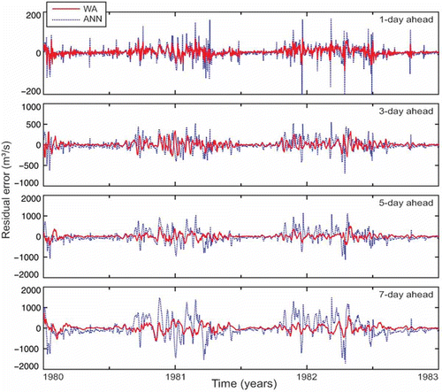
Fig. 9 Forecasting 1 day ahead with the ANN₁ model and WA₁ hybrid model compared with observed streamflow (Q_o).

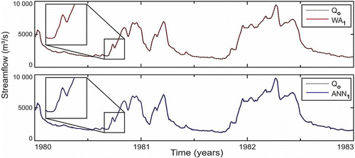
The results show that the forecast errors for WA models were always lower than those observed for ANN models and that the largest ones occurred for the highest flows. For 1- and 3-day ahead forecasts, the maximum residual error was –206.7 m³/s (2.4% of the observed value) for the ANN₁ model and –686 m³/s (8.7% of observed) for ANN₃, whereas it did not exceed –90.8 m³/s (1.0% of observed) for WA₁ and 336.4 m³/s (6.2% of observed) for WA₃. However, for more days ahead, the performance of the ANN models significantly decreased; in relative terms, the ANN₅ and ANN₇ models overestimated the forecast flows by 26% and 36%, respectively, while for the WA₅ and WA₇ models, these values were around 13% and 19%, respectively.

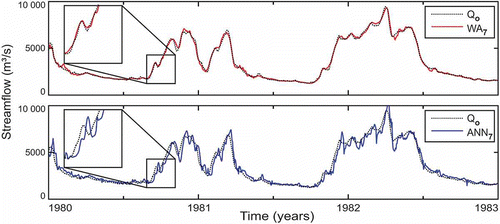
Observing the hydrographs in Fig. 10, the presence of small oscillations in the results obtained with the ANN₃ model is apparent. This type of instability was not observed for WA₃. It is also seen that the magnitude of these oscillations increased with the increase in forecast horizon (ANN₅ and ANN₇ models; Figs 11 and 12), whereas the results obtained with WA₅ and WA₇ models were stable. In addition, the 7-day ahead forecast obtained with ANN₇ seems to be noticeably lagged compared to the observed values. The same was not observed for the WA₇ model, which seems to be able to eliminate this tendency to lag. Note, from Table 3, that the inputs used in the WA₃, WA₅ and WA₇ models were the approximations A₃, A₄ and A₅, respectively. Such approximations contain no part of the high-frequency content, corresponding to details D₁, D₂ and D₃, extracted from the raw signal. With this, the oscillations and lags observed in the results of the ANN₃, ANN₅ and ANN₇ models, which used the raw flow time series as input, were avoided, improving the ANN forecasting capacity. However, it is important to be aware that the addition of more approximations to the input data does not necessarily improve the performance of WA models when the forecasting horizon increases, as has been discussed already.

Fig. 10 Forecasting 3 days ahead with the ANN₃ model and WA₃ hybrid model compared with observed streamflow (Q_o).

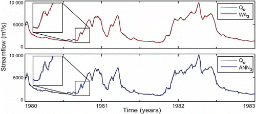
Fig. 11 Forecasting 5 days ahead with the ANN₅ model and WA₅ hybrid model compared with the observed streamflow (Q_o).

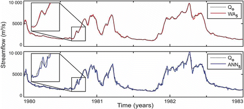
Fig. 12 Forecasting 7 days ahead with the ANN₇ model and WA₇ hybrid model compared with the observed streamflow (Q_o).

The same was not observed for 1-day ahead forecasts, where the best results were obtained when only the approximation A₁ was used as input to model WA₁. Using higher-level approximations (A₂, A₃,…), the forecasts obtained with WA₁ (not shown here) decreased significantly. These results revealed that, for the ANN to properly forecast short-term flows, it was necessary to keep practically all the content of the high-frequency signal (short-term oscillations) in the input information. Just the removal of detail D₁ was sufficient to improve the results. As D₁ also removes part of the noise present in the signal, this may be the reason why WA₁ performed better than ANN₁.

CONCLUSIONS

In this work, the performance of ANN models and wavelet–ANN hybrid models were compared for the 1-, 3-, 5- and 7-day ahead forecasts of daily streamflows. The WA models presented significantly better results than ANN models for all the situations tested. For short-term forecasting (1-day ahead), information about the high-frequency content of the signal was essential to ensure good model performance.

However, for more days ahead, the use of higher-order approximations, with less high-frequency content, were shown to be the most convenient input for WA hybrid models. These models were also found to be efficient in the elimination of the lags generally observed in the forecasting of daily flows by means of ANN models.

The results obtained here, although limited to a single application, demonstrate and quantify the benefits of wavelet transform use in the forecasting of daily streamflows by means of ANNs. The good performance of this hybrid approach is encouraging for the development of new research on this theme. It is believed that investigations in the sense of evaluating the influence of different mother-wavelet use in the development of WA models and the development of methods to select ANN input approximations may significantly contribute to the improvement of this approach.

Acknowledgements

The authors thank the ONS for the observed daily streamflow data provided.

Funding

The authors thank Brazil’s National Council for Scientific and Technological Development (CNPq) for financial support.

REFERENCES

- Abrahart, R.J., Heppenstall, A.J., and See, L.M., 2007. Timing error correction procedures applied to neural network rainfall–runoff modelling. Hydrological Sciences Journal, 52 (3), 414–431.
- Adamowski, J., 2007. Development of a short-term river flood forecasting method based on wavelet analysis. Warsaw: Polish Academy Sciences Monograph.
- Adamowski, J., 2008a. Development of a short-term river flood forecasting method for snowmelt driven floods based on wavelet and cross-wavelet analysis. Journal of Hydrology, 353, 247–266.
- Adamowski, J., 2008b. River flow forecasting using wavelet and cross-wavelet transform models. Hydrological Processes, 22, 4877–4891.
- Adamowski, J. and Sun, K., 2010. Development of a coupled wavelet transform and neural network method for flow forecasting of non-perennial rivers in semi-arid watersheds. Journal of Hydrology, 390, 85–91.
- Anctil, F. and Tape, D.G., 2004. An exploration of artificial neural network rainfall–runoff forecasting combined with wavelet decomposition. Journal of Environmental Engineering and Science, 3 (s1), s121–s128.
- ASCE Task Committee, 2000a. Artificial neural networks in Hydrology. I: preliminary concepts. Journal of Hydrologic Engineering, 5 (2), 115–123.
- ASCE Task Committee, 2000b. Artificial neural networks in hydrology II: hydrologic applications. Journal of Hydrologic Engineering, 5 (2), 124–132.
- Besaw, L.E., et al., 2010. Advances in ungauged streamflow prediction using artificial neural networks. Journal of Hydrology, 386, 27–37.
- Birikundavyi, S., et al., 2002. Performance of neural networks in daily streamflow forecasting. Journal of Hydrologic Engineering, 7 (5), 392–398.
- Bowden, G.J., Maier, H.R., and Dandy, G.C., 2005. Input determination for neural network models in water resources applications. Part 2. Case study: forecasting salinity in a river. Journal of Hydrology, 301, 93–107.
- Cannas, B., et al., 2006. River flow forecasting using neural networks and wavelet analysis. In: Proceedings of the European Geosciences Union. Munich: EGU Press.
- Chandramouli, V., et al., 2007. Backfilling missing microbial concentrations in a riverine database using artificial neural networks. Water Research, 41 (1), 217–227.
- Cigizoglu, H.K., 2004. Estimation and forecasting of daily suspended sediment data by multi-layer perceptrons. Advances in Water Resources, 27 (2), 185–195.
- Coulibaly, P. and Evora, N.D., 2007. Comparison of neural network methods for infilling missing daily weather records. Journal of Hydrology, 341, 27–41.
- Daliakopoulos, I.N., Coulibaly, P., and Tsanis, I.K., 2005. Groundwater level forecasting using artificial neural networks. Journal of Hydrology, 309 (1–4), 229–240.
- Daubechies, I., 1992. Ten lectures on wavelets. Philadelphia, PA: SIAM.
- Dawson, C.W., et al., 2006. Flood estimation at ungauged sites using artificial neural networks. Journal of Hydrology, 319 (1–4), 391–409.
- Dawson, C.W., Abrahart, R.J., and See, L.M., 2007. HydroTest: a web-based toolbox of statistical measures for the standardised assessment of hydrological forecasts. Environmental Modelling & Software, 27, 1034–1052.
- Dawson, C.W. and Wilby, R.L., 1999. A comparison of artificial neural networks used for river forecasting. Hydrology and Earth System Sciences, 3 (4), 529–540.
- Demuth, H. and Beale, M., 2005. Neural network toolbox: for use with Matlab. Natick, MA: The MathWorks.
- De Vos, N.J. and Rientjes, T.H.M., 2005. Constraints of artificial neural networks for rainfall–runoff modelling: trade-offs in hydrological state representation and model evaluation. Hydrology and Earth System Sciences, 9, 111–126.
- Elshorbagy, A. and Parasuraman, K., 2008. On the relevance of using artificial neural networks for estimating soil moisture content. Journal of Hydrology, 362, 1–18.
- Farias, C.A.S., Santos, C.A.G., and Celeste, A.B., 2011. Daily reservoir operating rules by implicit stochastic optimization and artificial neural networks in a semi-arid land of Brazil. In: G. Blöschl, et al., eds. Risk in water resources management. Wallingford: IAHS Press, IAHS Publication. 347, 191–197.
- Feng, S., et al., 2008. Neural networks to simulate regional ground water levels affected by human activities. Ground Water, 46 (1), 80–90.
- Guilhon, L.G.F., Rocha, V.F., and Moreira, J.C., 2007. Comparação de métodos de previsão de vazões naturais afluentes a aproveitamentos hidrelétricos. Revista Brasileira de Recursos Hídricos, 12 (3), 13–20.
- Haykin, S., 2005. Neural networks: a comprehensive foundation. New Delhi: Prentice-Hall.
- He, J., et al., 2011. Prediction of event-based stormwater runoff quantity and quality by ANNs developed using PMI-based input selection. Journal of Hydrology, 400, 10–23.
- Jain, A. and Srinivasulu, S., 2004. Development of effective and efficient rainfall–runoff models using integration of deterministic, real-coded genetic algorithms and artificial neural network techniques. Water Resources Research, 40, W04302.
- Jayawardena, A.W. and Fernando, T.M.K.G., 2001. River flow prediction: an artificial neural network approach. In: A.H. Schumann, et al., eds. Regional management of water resources. Wallingford: IAHS Press, IAHS Publication. 268, 239–245.
- Joorabchi, A., Zhang, H., and Blumenstein, M.M., 2007. Application of artificial neural networks in flow discharge prediction for the Fitzroy River, Australia. Journal Coastal Research, 50, 287–291.
- Kentel, E., 2009. Estimation of river flow by artificial neural networks and identification of input vectors susceptible to producing unreliable flow estimates. Journal of Hydrology, 375, 481–488.
- Kerh, T. and Lee, C.S., 2006. Neural networks forecasting of flood discharge at an unmeasured station using river upstream information. Advances in Engineering Software, 37 (8), 533–543.
- Kim, T.-W. and Valdés, J.B., 2003. Nonlinear model for drought forecasting based on a conjunction of wavelet transforms and neural networks. Journal of Hydrologic Engineering, 8 (6), 319–328.
- Kisi, Ö., 2007. Streamflow forecasting using different artificial neural network algorithms. Journal of Hydrologic Engineering, 12 (5), 532–539.
- Kisi, Ö., 2008. Stream flow forecasting using neuro-wavelet technique. Hydrological Processes, 22 (20), 4142–4152.
- Kisi, Ö., 2009. Neural networks and wavelet conjunction model for intermittent streamflow forecasting. Journal of Hydrologic Engineering, 14 (8), 773–782.
- Maier, H.R. and Dandy, G.C., 2000. Neural networks for the prediction and forecasting of water resources variables: a review of modelling issues and applications. Environmental Modelling & Software, 15 (1), 101–124.
- Mallat, S., 1989. A theory for multiresolution signal decomposition: the wavelet representation. IEEE Transactions Pattern Analysis and Machine Intelligence, 11 (7), 674–693.
- Muttil, N. and Chau, K.-W., 2006. Neural network and genetic programming for modelling coastal algal blooms. International Journal of Environment and Pollution, 28 (3/4), 223–238.
- Napolitano, G., Serinaldi, F., and See, L., 2011. Impact of EMD decomposition and random initialisation of weights in ANN hindcasting of daily stream flow series: an empirical examination. Journal of Hydrology, 406 (3–4), 199–214.
- Partal, T., 2009. River flow forecasting using different artificial neural network algorithms and wavelet transform. Canadian Journal of Civil Engineering, 36 (1), 26–38.
- Pulido-Calvo, I. and Portela, M.N., 2007. Application of neural approaches to one-step daily flow forecasting in Portuguese watersheds. Journal of Hydrology, 332, 1–15.
- Rajurkar, M.P., Kothyari, U.C., and Chaube, U.C., 2004. Modeling of the daily rainfall–runoff relationship with artificial neural network. Journal of Hydrology, 285, 96–113.
- Santos, C.A.G. and Morais, B.S., 2013. Identification of precipitation zones within São Francisco River basin by global wavelet power spectra. Hydrological Sciences Journal, 58 (4), 789–796. doi:10.1080/02626667.2013.778412.
- Santos, C.A.G., Morais, B.S., and Silva, G.B.L., 2009. Drought forecast using artificial neural network for three hydrological zones in San Francisco river basin. In: K.K. Yilmaz, et al., eds. New approaches to hydrological prediction in data-sparse regions. Wallingford: IAHS Press, IAHS Publication. 333, 302–312.
- Sarmiento, F.P. and Neira, N.O., 2009. Forecasting of monthly streamflows based on artificial neural network. Journal of Hydrologic Engineering, 14 (12), 1390–1395.
- Shrestha, R.R., Theobald, S., and Nestmann, F., 2005. Simulation of flood flow in a river system using artificial neural networks. Hydrology and Earth System Sciences, 9 (4), 313–321.
- Singh, K.P., et al., 2009. Artificial neural network modeling of the river water quality—a case study. Ecological Modelling, 220 (6), 888–895.
- Turan, M.E. and Yurdusev, M.A., 2009. River flow estimation from upstream flow records by artificial intelligence methods. Journal of Hydrology, 369, 71–77.
- Wang, W., Jin, J., and Li, Y., 2009. Prediction of inflow at Three Gorges Dam in Yangtze River with wavelet network model. Water Resources Management, 23 (13), 2791–2803.
- Wu, C.L., Chau, K.W., and Li, Y.S., 2009. Methods to improve neural network performance in daily flows prediction. Journal of Hydrology, 372, 80–93.