Regional models of flow-duration curves of perennial and intermittent streams and their use for calibrating the parameters of a rainfall–runoff model

Abstract

One of the main challenges faced by hydrologists and water engineers is the estimation of variables needed for water resources planning and management in ungauged river basins. To this end, techniques for transposing information, such as hydrological regional analyses, are widely employed. A method is presented for regionalizing flow-duration curves (FDCs) in perennial, intermittent and ephemeral rivers, based on the extended Burr XII probability distribution. This distribution shows great flexibility to fit data, with accurate reproduction of flow extremes. The performance analysis showed that, in general, the regional models are able to synthesize FDCs in ungauged basins, with a few possible drawbacks in the application of the method to intermittent and ephemeral rivers. In addition to the regional models, we summarize the experience of using synthetic FDCs for the indirect calibration of the Rio Grande rainfall–runoff model parameters in ungauged basins.

Editor D. Koutsoyiannis

Citation Costa, V., Fernandes, W., and Naghettini, M., 2013. Regional models of flow-duration curves of perennial and intermittent streams and their use for calibrating the parameters of a rainfall–runoff model. Hydrological Sciences Journal, 59 (2), 262–277.

Résumé

L’une des principales difficultés rencontrées par les hydrologues et les ingénieurs dans le domaine de l’eau est l’estimation des variables nécessaires à la planification et à la gestion des ressources en eau dans des bassins fluviaux non jaugés. A cette fin, les techniques de transposition de l’information, telles que les analyses hydrologiques régionales, sont largement utilisées. Nous présentons une méthode de régionalisation des courbes de débits classés pour les rivières pérennes, intermittentes et saisonnières, basée sur la distribution de probabilité étendue de Burr XII. Cette distribution présente une grande flexibilité pour s’ajuster aux données, avec une reproduction précise des extrêmes de débit. L’analyse des performances a montré qu’en général, les modèles régionaux sont capables de synthétiser des courbes de débits classés dans les bassins versants non jaugés, avec quelques inconvénients possibles dans l’application de la méthode aux rivières intermittentes et saisonnières. En plus des modèles régionaux, nous résumons l’expérience d’utilisation des courbes de débits classés synthétiques pour le calage indirect des paramètres du modèle pluie-débit du Rio Grande pour des bassins versants non jaugés.

Key words:

• regional models
• flow-duration curve
• extended Burr XII probability distribution

Mots clefs:

• modèles régionaux
• courbe des débits classés
• distribution de probabilité
• étendue de Burr XII

1 INTRODUCTION

Flow-duration curves (FDCs) represent the relationship between magnitude and frequency of streamflow, determining the percentage of a given time span that a specified flow is equalled or exceeded. FDCs are usually computed from daily flow records and may refer either to the annual time span or to a historical multi-year period of record. Alternatively, one can interpret an FDC as the complement of the cumulative distribution function of streamflows.

Flow-duration curves are a simple representation of the hydrological response of a river basin: their shape and slope express streamflow variability and are functions of physical, climatological, morphological and land-use characteristics. The area under the curve represents the total runoff volume in the period of record.

A wide range of uses are associated with FDCs: water availability studies, hydropower generation and reservoir operation, water quality assessment (Cole et al. 2003), hydrological regional analysis (Mohamoud 2008) and, more recently, the indirect calibration of the parameters of rainfall–runoff models (Liu and Han 2010, Pinheiro and Naghettini 2010, Westenberg et al. 2011, Prafulla et al. 2012).

Flow-duration curves can be constructed by means of two distinct approaches. In the first, all data from the period of record are used and the curve is referred to as a long-term FDC. The probabilistic interpretation of an FDC is restricted to the period of record and its use is only recommended when this period is long enough to characterize the streamflow limiting distribution. Despite these limitations, FDCs can be used to fill missing data and also to generate synthetic flow series in ungauged basins through the use of a regional model (Hughes and Smakhtin 1996).

In the second approach, construction of the curves is carried out for every year (calendar or hydrological) and the curves are termed annual AFDCs. The use of this approach has been increasing because it allows a conventional statistical treatment: inter-annual variability can be evaluated and recurrence intervals can be associated with the curves. Furthermore, one can construct a median AFDC, representative of a median hypothetical year, supposedly not affected by abnormally wet or dry periods.

Independent of the approach used, FDCs are constructed by ranking the daily streamflows and assigning an exceedence probability to each ranked flow. Several estimators can be used for this purpose (Vogel and Fenessey 1994); the most common is based on the Weibull plotting position, which expresses the exceedence probability as follows:

(1)

where i denotes the rank of a given flow and n is the total number of flow records.

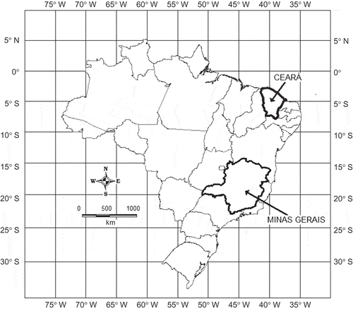
This study presents a method for identifying a regional model of FDCs sufficiently general to represent the hydrological regimes of perennial and intermittent rivers. The models are based on the extended Burr XII distribution, which is characterized by its greater flexibility of shape and its goodness of fit to empirical data. The regional models were applied to catchments located in the Brazilian states of Minas Gerais and Ceará, as shown in Fig. 1, encompassing perennial, intermittent and ephemeral streams. In addition, the experience of using synthetic FDCs for the indirect calibration of parameters for the Rio Grande rainfall–runoff model in ungauged basins is summarized, thus enabling a wide range of hydrological analyses in both regions under study.

Fig. 1 The Brazilian states, Minas Gerais and Ceará, in which the basins employed in the study are located.

2 CONSTRUCTION OF FDCS USING THE TOTAL PROBABILITY THEOREM

The use of conventional techniques for the construction of FDCs in intermittent and ephemeral rivers is not possible due to zero flows. To solve this problem, Haan (1977, in Crocker et al. 2003) suggested the use of the total probability theorem, according to which the probability of an event A, belonging to the sample space S consisting of K mutually and collectively exclusive events B_i, with i ≤ K, is given by:

(2)

For streamflow, the sample space consists of zero and non-zero flows. Thus:

(3)

Since , it follows that:

(4)

Considering the duration as the complement of the cumulative distribution function, one can express equation (4) as follows:

(5)

where p^*(i) corresponds to non-zero flow durations and p(i) corresponds to all flow durations. Equation (5) shows that the term p(Q > 0) acts like an adjustment for non-zero flow durations. More recently, Rianna et al. (2011) employed a similar approach to develop a stochastic index model to regionalize FDCs for intermittent rivers.

3 THE EXTENDED BURR XII DISTRIBUTION FUNCTION FOR MODELLING FDCs

Burr (1942) introduced a system of cumulative distribution functions, based on the following differential equation:

(6)

The solution of equation (6) is expressed as follows:

(7)

where g(x) is a function that makes F(x) vary between 0 and 1, while x varies between –∞ and +∞.

Burr (1942) proposed a family of 12 particular solutions for equation (7), highlighting the so-called type XII, given by:

(8)

where c and K ≥ 1 are shape parameters of the distribution.

Shao et al. (2004) proposed a reparameterization of the original form of the Burr XII distribution, aiming to achieve greater flexibility in fitting empirical data. They termed this new form of the distribution “the extended Burr XII distribution”, although, according to Nadarajah and Kotz (2006), this model can also be referred to as the generalized Weibull distribution. In this reparameterization, the cumulative distribution function F(x) is expressed as follows:

(9)

where α = 1/c, β = –K and λ = –b/β^α.

Shao et al. (2009) successfully applied the extended Burr XII to model FDCs in Australian catchments encompassing perennial, intermittent and ephemeral streams. However, we could not find regionalization works that used this distribution in our literature review. Thus, we describe a full application of the extended Burr XII distribution herein, both as a regional model for FDCs in perennial and intermittent rivers, and for the indirect calibration of the parameters describing a particular rainfall–runoff model, namely the Rio Grande model.

The FDC models derived from the extended Burr XII distribution can be expressed by:

(10)

where Q_p denotes the streamflow associated with duration p; λ is the scale parameter; α and β are shape parameters; and τ represents the fraction of time during which non-zero flows occur in the river. Parameter τ is termed “cease-to-flow” by Shao et al. (2009); in perennial streams, τ = 1.

It is worth understanding how these parameters affect the FDC. The cease-to-flow parameter τ changes the right end-point of the FDC, while the scale parameter λ changes it proportionally. When β ≥ 1, an increase in α will make the FDC steeper, whereas, for β < 1, an increase in α will shift the high-flow section of the FDC upwards and the low-flow section downwards. An increase in β will make the FDC steeper, particularly for the largest discharges (Shao et al. 2009).

4 FDC REGIONAL MODELS AND PERFORMANCE ANALYSIS

The construction of FDCs followed a statistical approach, in which extended Burr XII parameters, estimated at each gauging station, are related to physical, climatological and morphological characteristics of basins by means of multiple linear regression. Hereafter, these regression models are termed complete regional models (CRMs).

Following identification of the CRMs, performance and reliability analyses were carried out. In this regard, the “jack-knife” cross-validation procedure was used, as suggested by Castellarin et al. (2004). In short, the cross-validation consists of the following steps:

1. A regional model is identified for the set of N streamgauges in the study region.

2. A given gauging station, denoted by s, is removed from the set.

3. A new regional model, termed a jack-knife model (JKM), is then built on the basis of the set of remaining N – 1 streamgauges, using the same explanatory variables as obtained in Step 1.

4. The regional model identified in Step 3 is used to estimate the synthetic FDC for station s.

5. Steps 2–4 are repeated until all the stations have been removed from the set.

6. Finally, each of the N synthetic FDCs is compared with the observed FDC, using the following performance indices:

1. the relative error ε_s,j at station s, associated with duration j:

   (11)

   where denotes the flow obtained from the regional models, corresponding to duration j, and q_s,j denotes the flow as read in the observed FDC, corresponding to duration j;

2. the mean relative error at station s:

   (12)

   in which N_D denotes the number of durations used in the computation of relative errors;

3. the standard deviation of relative errors :

   (13)

4. the Nash-Sutcliffe efficiency coefficient:

   (14)

where denotes the mean flow at station s.

In addition to the above indices, the p descriptors were evaluated. These descriptors express the percentage of cases, with respect to N, for which E_s > 0.75 (p₁: good to fair fit), 0.50 < E_s < 0.75 (p₂: fair to poor fit) and E_s < 0.50 (p₃: poor fit).

5 THE RIO GRANDE RAINFALL–RUNOFF MODEL

5.1 Introduction

The Rio Grande model is a conceptual, semi-distributed rainfall–runoff model, which incorporates current solutions to the mathematical modelling of hydrological processes. It comprises a runoff production module, a flow concentration module and a flow routing module.

5.1.1 Runoff production module

This module is based on the concept of the Xinanjiang model, first described by Zhao et al. (1980). The main characteristic of the Xinanjiang model derives from the concept that runoff occurs only when the nominal maximum soil moisture storage is reached. In other words, runoff is not produced until the soil moisture content of the aeration zone reaches field capacity.

Soil, like any porous medium, has the ability to retain a certain amount of water against the force of gravity. The maximum capacity of soil moisture storage is sometimes referred to as the field capacity. Water retained by capillary forces cannot become runoff and can only be depleted by soil evaporation or plant transpiration. According to Zhao (1980), evapotranspiration is the main controlling factor of how soil moisture storage depletes over time.

A flow chart of the runoff production module is shown in Fig. 2. All symbols inside the blocks are variables (inputs, outputs and internal variables), while those outside the blocks are parameters. It follows the main elements of the Xinanjiang model (Zhao et al. 1980), incorporating some minor changes as adopted in the Rio Grande model formulation.

Fig. 2 Flow chart of the runoff production module of the Rio Grande model, which is similar to the Xinanjiang model described by Zhao et al. (1980).

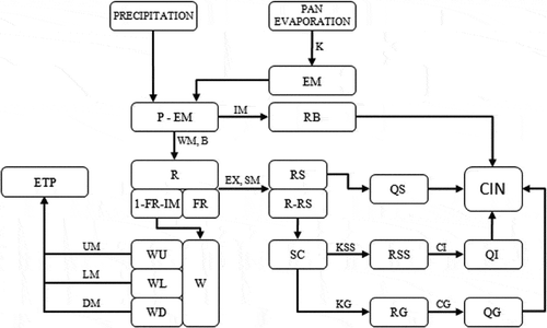
In Fig. 2, the model input variables are the mean areal precipitation (P) and daily pan evaporation (EM), and the main output is the total discharge per unit area (CIN) (in mm km^-2 d^-1).

The state variables are the mean spatial soil water (W), representing the water storage, and the mean spatial free water storage (S), representing the amount of water in the soil that is free to flow, where W has three components, WU, WL and WD, representing the water storage in the upper, lower and deep layers, respectively; FR is the runoff contributing area factor, which is related to W; RB is the runoff from the usually small portion of impermeable area; and R denotes the runoff yield of the permeable area, formed by surface (RS), interflow (RSS) and groundwater (RG) runoff components, each of which reaches the drainage system at different velocities. Therefore, the runoff components are transferred into QS, QI and QG, respectively, and together form the total inflow to the channel network of the sub-basin (CIN).

As mentioned above, the symbols outside the blocks in Fig. 2 denote parameters: K is the ratio of potential evapotranspiration to pan evaporation; WM and B describe the soil water distribution, where WM is the mean spatial soil water capacity, having components UM, LM and DM, and B is the exponent of the soil water capacity distribution curve; IM is the impermeable area factor; SM and EX describe the distribution of free water capacity, where SM is the mean spatial free water storage capacity and EX is the exponent of the free water capacity curve; KG and KSS are the outflow coefficients of the free water storage to groundwater and interflow, respectively; and, finally, CG is the daily recession constant of the groundwater flow and CI is the recession constant of the interflow.

For more details on the meaning and typical values of these parameters, the reader is referred to Zhao et al. (1980).

5.1.2 Flow concentration module

The total inflow to the channel network of the sub-basin (CIN) represents the flow generated in the basin per unit area. However, it has to be pointed out that the flow generated in different areas of the basin is concentrated at the main outlet with different time lags. In the Rio Grande model, this is dealt with by applying a transfer function based on Clark’s synthetic unit hydrograph, as originally formulated by the Hydrological Engineering Center of the US Army Corps of Engineers (Hydrological Engineering Center 1981).

5.1.3 Flow routing module

The flow routing in the Rio Grande model is based on the diffusive wave model, as suggested by Cunge (Ponce 1989), commonly referred to as the Muskingum-Cunge model. In the application described herein, the Rio Grande model was used in its lumped version and the flow routing module was not employed.

5.2 Indirect calibration using synthetic FDCs

In regionalization studies, it is usual for rainfall–runoff model parameters to be related to physical, climatological and morphological characteristics of the catchment. The drawbacks of this methodology are: the great number of parameters to be regionalized, the correlation between parameters, the difficulty of associating parameters with catchment characteristics and the existence of multiple sets of parameters providing reasonably satisfactory results (Vogel 2006).

Yu and Yang (2000) suggested a methodology for hydrological models calibration using synthetic FDCs. The main idea is to find a set of parameters able to synthetize the ranked flows, with no obligation to reproduce their serial structure (Pinheiro and Naghettini 2010). This structure is retrieved indirectly, through the evolution of rainfall and evaporation over the simulation period. The main advantage of this method is that only the parameters of the distribution function that models the FDC are regionalized.

In this paper, indirect calibration methodology was used for a number of analyses involving the Rio Grande rainfall–runoff model. For perennial streams, a comparative evaluation of parameter calibration quality (Colischonn et al. 2007), as mimicking the long-term FDC or the median AFDC as the main goal of calibration, was carried out. For intermittent and ephemeral streams, calibration was carried out only for FDCs (Pilgrim et al. 1988, De Boer 1992, Hughes 1995). The main objective was to assess the ability of the Rio Grande model to reproduce the flow intermittence condition, since its original structure had not been designed for this particular purpose. The assessment of parameter calibration quality was performed using the following indices:

1. The Nash-Sutcliffe efficiency criterion, E:

   (15)

   where i is time in days; N is the number of days of calibration, with the exception of the model warm-up period; Q_obs,i represents the observed flow on day i; Q_sim,i denotes the simulated flow on day i and is the mean observed flow;

2. the root mean square error, RMSE:

   (16)

3. the average absolute percent error, AAPE:

   (17)

Finally, two other indices were used: the K index, which is the ratio between the flow volumes as calculated for the calibrated and observed hydrographs over the full period of calibration (except for the first-year warm-up period), and the squared correlation coefficient (R²) between simulated and observed flows, which gives a summary of the concordance between simulated and observed flows, as well as the time coherence between them.

6 APPLICATION OF THE METHODOLOGY TO PERENNIAL STREAMS IN MINAS GERAIS

6.1 Identification of regional FDCs

The basins of the Pará and the Paraopeba rivers are right-bank tributaries of the Upper San Francisco River. Regional models were identified for FDCs and median AFDCs in these basins. These models will be used later in the calibration of the Rio Grande rainfall–runoff model. Ten stream gauging stations were selected for the identification of regional models, with a common period of 29 years of record. The stations and the main attributes of the sub-basins are presented in Table 1.

Table 1 Streamflow gauging stations and physical, climatological and morphological characteristics of the basins in Minas Gerais (A: drainage area of basin, L: length of main stream in basin, H_max: watershed maximum elevation, H_min: watershed minimum elevation, k_c: watershed compactness coefficient, k_f: watershed shape coefficient, P: mean annual rainfall, C_esc: runoff coefficient of the basin, given by the relationship between runoff volume and rainfall volume, DD: drainage density, S_eq: equivalent slope).

Stationcode	A(km^2)	L(km)	Hmin(m)	Hmax(m)	kf	kc	P(mm)	Cesc	DD(junc./km^2)	Seq(m/km)
40130001	1620	75.8	759	1160	0.30	1.47	1533	0.33	0.114	1.92
40300001	1558	119.1	656	1100	0.11	1.70	1432	0.31	0.099	1.82
40330000	7378	219.4	609	1160	0.15	1.66	1456	0.30	0.036	0.75
40450001	11302	293.1	589	1160	0.13	1.71	1431	0.29	0.054	0.46
40549998	461	52.0	877	1140	0.17	1.52	1400	0.38	0.098	2.69
40680000	486	47.3	863	1100	0.22	1.34	1369	0.44	0.136	1.25
40710000	2760	118.9	794	1140	0.20	1.28	1408	0.40	0.137	1.59
40740000	3939	187.4	736	1140	0.11	1.49	1422	0.35	0.134	1.21
40800001	5680	236.3	703	1140	0.10	1.64	1449	0.33	0.141	1.00
40865001	10192	419.8	633	1140	0.06	1.87	1414	0.33	0.133	0.60

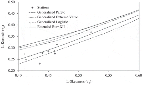
The suitability of the extended Burr XII probability distribution for representing the empirical FDCs and median AFDCs was graphically evaluated with the use of L-moment ratio diagrams (Castellarin et al. 2007). Figure 3 shows this diagram for the data used in the construction of FDCs. From the three-parameter distributions fitted in this diagram, one can observe that the extended Burr XII is a plausible candidate for the purposes of modelling the empirical FDCs, although the Generalized Pareto distribution could also be used for that purpose. In this context, other flexible models, such as the four-parameter Kappa, the Wakeby and the generalized gamma distributions, could also be included, and eventually chosen, as good candidate models on the basis of a comparative goodness of fit. Similar results, not shown here, were obtained for median AFDCs.

Fig. 3 L-moment ratio diagram for FDCs in Minas Gerais.

The parameters of the extended Burr XII probability distribution were estimated by the method of L-moments (MML). The parameters were related to the catchment characteristics through multiple linear regression. Regression equations for each parameter are shown in Table 2 (FDC) and Table 3 (AFDC), along with the values of the coefficient of determination, the adjusted coefficient of determination, the standard error and the F_total statistic.

Table 2 Regression equations for the parameters of the extended Burr XII distribution for FDCs (R²: coefficient of determination; R²_adj: adjusted coefficient of determination).

Regional equation	R^2	R^2adj.	Standard error	Ftotal
λ = 0.02003A^0.97077kc^-1.01951	0.99	0.99	0.055	1680
α = –3.23919 + 0.0008Hmax + 0.4406kc + 0.00075P + 2.40647Cesc	0.88	0.78	0.024	8.8
β = –78.24 + 11.409ln(Hmax) + 0.434ln(kf) + 5.558ln(kc) + 5.327ln(Cesc)	0.91	0.83	0.141	12.2

Table 3 Regression equations for the parameters of the extended Burr XII distribution for median AFDCs (R²: coefficient of determination; R²_adj: adjusted coefficient of determination).

Regional equation	R^2	R^2adj.	Standard error	Ftotal
λ = 0.018A^0.98kc^-1.15	0.99	0.99	0.129	312.5
α = 0.55 + 0.17(1/Seq) – 590.40(1/(Hmin) – 0.003(1/DD) + 0.126(1/Cesc)	0.90	0.82	0.020	10.9
β = –2.08 –0.15(1/DD) + 1.97(1/Seq) – 0.14(1/kf) + 437.08(1/A)	0.89	0.80	0.420	10.0

6.2 Performance analysis of regional models for FDCs

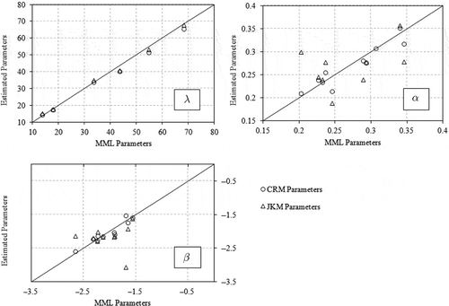
As mentioned previously, the performance analysis was based on the cross-validation procedure suggested by Castellarin et al. (2004). Figure 4 shows scatter plots of the CRM parameters and JKMs of FDCs in comparison to the MML estimates. One can see that the scatter is not high, indicating that the loss of information resulting from the removal of one station does not significantly affect the performance of the JKMs. This result suggests the robustness of the proposed methodology.

Fig. 4 Scatter plots of CRM and JKM parameters in comparison to MML estimates.

The performance indices for the set of 99 durations in the interval [1–99]% were calculated for the JKM models for FDCs; for all stations, E_s > 0.75 (p₁ = 100%). In addition, the scatter of the errors as the catchment drainage area varies was evaluated (not shown here). No trends were observed, indicating that the regional models have no bias as far as scale is concerned.

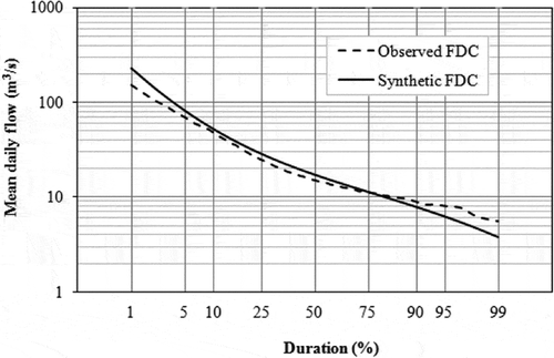
Finally, the correspondence between the synthetic and observed FDCs at Jaguaruna gauging station (Fig. 5) shows the quality of the obtained results, as this had the worst performance among the 10 stations.

Fig. 5 Comparison between synthetic and observed FDCs at Jaguaruna station (40300001).

As an illustration, performance indices were also computed for the CRM and MML models. The results for the FDCs are presented in Table 4, showing excellent goodness-of-fit measures provided by the extended Burr XII distribution function, as indicated by the low values of mean relative error, ε_s, and high Nash-Sutcliffe efficiency criterion, E. The performance of the JKMs is not significantly lower than that of the CRMs, which is clear evidence of the robustness and reliability of the proposed method.

Table 4 Performance indices for the three parameter estimation methods for FDCs (MML: method of L-moments; CRM: complete regional model; JKM: jack-knife model).

Station	MML			CRM			JKM
	εs	σe,s	Es	εs	σe,s	Es	εs	σe,s	Es
40130001	0.0006	0.059	0.973	–0.0264	0.059	0.950	–0.0039	0.085	0.979
40300001	–0.0141	0.080	0.985	0.0072	0.077	0.962	0.0822	0.129	0.823
40330000	–0.0246	0.090	0.955	–0.0613	0.084	0.946	–0.0228	0.083	0.963
40450001	–0.0014	0.080	0.957	0.0148	0.127	0.944	0.0712	0.193	0.884
40549998	0.0015	0.053	0.985	–0.0812	0.051	0.964	–0.0878	0.059	0.947
40680000	–0.0028	0.050	0.990	–0.0072	0.065	0.989	0.0390	0.108	0.981
40710000	–0.0092	0.076	0.990	–0.0108	0.069	0.978	0.0214	0.077	0.958
40740000	–0.0117	0.068	0.986	–0.0782	0.050	0.976	–0.0514	0.057	0.974
40800001	0.0004	0.061	0.978	–0.0345	0.062	0.938	0.0053	0.069	0.891
40865001	–0.0098	0.080	0.979	–0.1036	0.074	0.945	–0.0870	0.081	0.931
p descriptors	p1	100.00		p1	100.00		p1	100.00
	p2	0.00		p2	0.00		p2	0.00
	p3	0.00		p3	0.00		p3	0.00

As for the AFDCs, similar performance analyses were made. The results were slightly inferior to those achieved for the FDCs, with relatively poorer fits in the lower and upper tails. The results for the AFDC fits are summarized in Table 5.

Table 5 Performance indices for the three parameter estimation methods for median AFDCs.

Station	MML			CRM			JKM
	εs	σe,s	Es	εs	σe,s	Es	εs	σe,s	Es
40130001	–0.030	0.034	0.987	–0.026	0.048	0.982	–0.125	0.088	0.965
40300001	0.107	0.091	0.989	–0.032	0.192	0.705	–0.002	0.357	0.257
40330000	–0.093	0.093	0.967	0.115	0.106	0.945	0.063	0.105	0.951
40450001	0.106	0.118	0.977	–0.065	0.098	0.927	–0.040	0.087	0.940
40549998	–0.012	0.064	0.954	–0.108	0.137	0.941	–0.169	0.138	0.875
40680000	0.028	0.092	0.984	–0.009	0.096	0.977	–0.003	0.050	0.989
40710000	0.001	0.055	0.992	0.073	0.058	0.980	0.202	0.064	0.889
40740000	–0.003	0.062	0.990	0.073	0.132	0.874	0.090	0.154	0.811
40800001	–0.004	0.075	0.964	–0.006	0.094	0.831	–0.003	0.105	0.770
40865001	0.026	0.088	0.975	0.005	0.077	0.962	–0.039	0.076	0.947
p descriptors	p1	100.00		p1	100.00		p1	90.00
	p2	0.00		p2	0.00		p2	0.00
	p3	0.00		p3	0.00		p3	0.00

6.3 Calibration of the Rio Grande rainfall–runoff model using FDCs modelled by the extended Burr XII distribution

The parameter calibration of the Rio Grande rainfall–runoff model in the watersheds aimed to allow assessment of calibrations having FDCs as the main object of calibration compared to median AFDCs. Only the watersheds of perennial rivers in Minas Gerais state were employed for this purpose. The main input data to the model are: drainage area and dominant shape of the catchment (circular, rectangular or ellipsoidal); daily rainfall and evaporation; and attributes of the objective function, such as the duration to be evaluated and the number of iterations. The main information used to calibrate the model is the JKM parameters for FDCs and median AFDCs.

Calibration was performed for the period from October 1992 to September 1998. In the calculation of performance indices, the first year, corresponding to the “warm-up” period of the Rio Grande model, was removed from the analysis. Tables 4 and 5 show the performance indices of hydrographs for calibrations with FDCs and median AFDCs, respectively.

Tables 6 and 7 show that the calibration with median AFDCs performs better than that with FDCs. In the first case, the Rio Grande simulation was able to explain about 59.5% of the total variance of flows, whereas in the latter case the corresponding value was 48.2%. Also, for calibration with median AFDCs, the K index is closer to unity, showing the better reproduction of observed flow volumes. The AAPE and R² values were similar for both cases (Tables 6 and 7).

Table 6 Performance indices for hydrographs simulated by the Rio Grande model, as calibrated with long-term flow-duration curves (FDCs).

Station	RMSE	AAPE	E	K	R^2
40130001-2	28.642	0.301	0.197	1.193	0.861
40300001	14.258	0.181	0.641	1.061	0.766
40330000	76.695	0.200	0.541	1.113	0.884
40450001	115.092	0.184	0.365	1.226	0.893
40549998	7.447	0.304	0.232	1.034	0.692
40680000	14.219	0.338	0.642	0.860	0.659
40710000	43.080	0.322	0.380	1.049	0.698
40740000	72.844	0.243	-0.246	1.150	0.832
40800001	61.514	0.221	0.563	1.053	0.801
40865001	84.103	0.207	0.781	1.069	0.890
Mean	51.789	0.250	0.482*	1.081	0.798

*Excluding station 40740000.

Table 7 Performance indices for hydrographs simulated by the Rio Grande model, as calibrated with median annual flow-duration curves (AFDCs).

Station	RMSE	AAPE	E	K	R^2
40130001-2	26.479	0.311	0.313	1.184	0.872
40300001	19.293	0.234	0.598	1.159	0.784
40330000	61.564	0.198	0.762	1.099	0.875
40450001	79.639	0.251	0.739	1.126	0.868
40549998	6.900	0.312	0.395	1.032	0.681
40680000	10.482	0.302	0.729	0.871	0.839
40710000	43.986	0.312	0.569	1.048	0.713
40740000	51.653	0.235	0.569	1.089	0.799
40800001	59.632	0.184	0.592	1.041	0.823
40865001	86.913	0.298	0.682	1.121	0.840
Mean	44.654	0.264	0.595	1.077	0.809

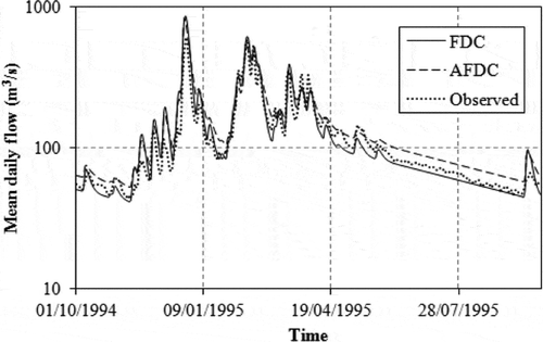
Figure 6 shows a comparison of hydrographs simulated by the model calibrated with the FDC and the median AFDC, and the observed hydrograph for the hydrological year 1 October 1994–30 September 1995, at the gauging station of Porto Pará (40450001). In Fig. 6, the calibration with the FDC fits the receding flows better, whereas slightly larger values of E and smaller RMSEs (see Tables 6 and 7) indicate that the median AFDC fits the hydrograph peaks better. The same result was observed for all gauging stations in the study region.

Fig. 6 Comparison between the hydrographs simulated by the model calibrated with the FDC and the median AFDC, and the observed hydrograph at Porto Pará gauging station for the hydrological year 1994/95.

7 APPLICATION OF THE METHODOLOGY TO INTERMITTENT AND EPHEMERAL STREAMS IN CEARÁ STATE

7.1 Identification of regional FDCs

The watersheds selected for this study, located in the state of Ceará in the semi-arid Northeast region of Brazil, are of the intermittent rivers Poti, Banabuiú, Jaguaribe, Acaraú and Salgado. Regional models were identified only for FDCs in these basins; these will be used later in the indirect calibration of the Rio Grande rainfall–runoff model. The data observation periods range from 13 to 62 years. Eight gauging stations were used to build the regional models. The stations and the main attributes of the sub-basins are given in Table 8.

Table 8 Streamflow gauging stations and physical, climatological and morphological characteristics of the basins in Ceará (A: drainage area of basin, L: length of the main stream in basin, CTD: total length of drainage in basin, P: mean annual rainfall, C_esc: runoff coefficient of the basin, C_ris: watershed percent area located on fractured rock aquifer).

Station code	A (km^2)	L (km)	CTD (m)	P (mm)	Cesc	Cris (%)
34750000	18340	255	12526	945	0.066	85.1
35210000	1643	120	1624	780	0.189	100.0
36125000	3746	139	2353	738	0.053	67.2
36210000	1756	121	1156	1041	0.070	18.5
36250000	4372	157	3105	887	0.032	24.4
36290000	12680	176	11203	928	0.080	59.0
36470000	4838	142	4102	764	0.109	100.0
35260000	2818	155	2653	720	0.16	99.6

The suitability of the extended Burr XII distribution for representing the empirical FDCs was evaluated graphically using L-moment ratio diagrams (not shown here). The shape and scale parameters of the extended Burr XII distribution function were estimated by the MML. The parameter τ is the percentage of time in which there is non-zero flow in the river. All four distribution parameters were related to physical, climatological and morphological characteristics of the catchments through multiple linear regression, and the regression equations for each parameter are presented in Table 9.

Table 9 Regression equations for the parameters of the extended Burr XII distribution function for FDCs.

Regional equation	R^2	R^2adj.	Standard error	Ftotal
λ = 0.1817CTD^0.5453Cesc^0.6463	0.93	0.91	0.576	34.7
α = 1.4916 – 0.0054CT + 0.0130Cris	0.92	0.88	0.209	27.5
β = –0.6849 – 0.000041CTD + 0.0043Cris	0.89	0.85	0.096	20.6
τ = 1.3601 – 0.0104P^0.5 + 0.0050CTD^0.5 – 0.0863Cris^0.5	0.87	0.78	1.163	9.2

7.2 Performance analysis of the regional models for FDCs

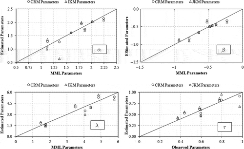
Figure 7 depicts scatter plots of the parameter estimates by the CRM and the JKM vs the MML estimates. The scatter is not great for any of the parameters; however, for some values of τ, scatter is significant. For example, for station 36290000, the, observed τ is 0.972 while the predicted value is 0.683.

Fig. 7 Scatter plots of CRM and JKM parameters vs MML estimates.

Due to the poor estimates found for parameter τ, the performance of the methodology was not as good as for the watersheds in the state of Minas Gerais (perennial rivers). For three gauging stations, the E_s index was smaller than 0.50. In addition, the relative errors are extremely high in the low-flow portion of the FDCs, which parameter τ affects most.

Due to the sensitivity of flow estimates, performance indices were also calculated for the observed values of parameter τ, keeping the jack-knife estimates of the other parameters. A significant reduction in the values of the relative errors was observed. Furthermore, only one station presented E_s in the intermediate range, which shows, on the one hand, the robustness of the regional models for this situation, and on the other hand, the need for more reliable estimates for τ.

Figure 8 shows the comparison of synthetic and observed FDCs for estimated and observed values of parameter τ at the gauging station of Sítio da Lapinha (36210000).

Fig. 8 Comparison between synthetic and observed FDCs at Sítio da Lapinha station (36210000) for estimated τ (a) and observed τ (b).

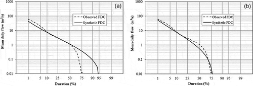
The variation of the errors with catchment drainage area was also evaluated, but no trends were observed. However, the errors associated with the estimated values of τ were much larger than those associated with observed τ. As an illustration, performance indices were calculated for CRM and MML models, taking into account the estimated and observed values of parameter τ (Table 10).

Table 10 Performance indices of FDC models for intermittent streams in Ceará state.

Station	MML models			CRM τobs			CRM τest			JKM τobs			JKM τest
	εs	σe,s	Es	εs	σe,s	Es	εs	σe,s	Es	εs	σe,s	Es	εs	σe,s	Es
34750000	0.081	0.27	0.96	0.064	0.30	0.82	0.514	1.88	0.07	1.426	6.23	0.85	3.992	20.11	0.09
35210000	–0.092	0.30	0.98	–0.113	0.27	0.95	1.038	3.50	0.96	–0.185	0.24	0.89	2.153	8.27	0.88
35260000	–0.075	0.22	0.95	–0.126	0.23	0.95	–0.612	0.29	0.89	–0.129	0.24	0.98	0.101	0.20	0.97
36110000	–0.089	0.29	0.97	0.178	0.35	0.92	–0.248	0.38	0.99	0.303	0.39	0.94	–0.481	0.36	0.97
36125000	0.179	0.51	0.98	0.189	0.72	0.93	1.299	3.54	0.95	0.051	0.41	0.95	2.414	6.77	0.89
36210000	0.389	1.27	0.98	0.257	1.28	0.99	1.053	3.55	0.98	–0.156	0.46	0.91	4.252	11.99	0.98
36290000	0.045	0.36	0.92	0.149	0.49	0.82	0.508	0.40	0.59	0.194	0.53	0.87	–0.549	0.42	0.46
36470000	–0.094	0.25	0.99	–0.135	0.24	0.94	2.648	4.34	0.91	–0.138	0.24	0.68	3.842	6.55	0.45
p descriptors	p1	100.0		p1	100.0		p1	75.0		p1	87.5		p1	62.5
	p2	0.0		p2	0.0		p2	0.0		p2	12.5		p2	0.0
	p3	0.0		p3	0.0		p3	25.0		p3	0.0		p3	37.5

Analysis of Table 10 shows that mean relative errors for the Ceará watersheds are larger than those for the Minas Gerais watersheds. This fact is largely attributed to the difficulty of modelling the low flow portions of FDCs for intermittent and ephemeral streams. The influence of parameter τ in the performance of CRMs and JKMs is evident. We conclude that the robustness of the methodology is directly related to good estimates of parameter τ. When observed τ values are employed, the performance results are satisfactory and comparable to those obtained for perennial streams, thus showing the reliability and robustness of the method under this condition.

7.3 Calibration of Rio Grande rainfall–runoff model using FDCs modelled with the extended Burr XII distribution function

Calibration of the Rio Grande model parameters for the Ceará watersheds aimed to assess the model’s ability to reproduce the stream intermittence condition in this semi-arid region. In order to accomplish this without drastically changing the model structure, the soil water reservoirs of the Rio Grande model, as described by the variation bounds for parameters W, WU, WL and WD (see Section 5.1), were made larger so that more capillary water would be lost by evapotranspiration, thus reducing the water available for sub-surface flow and baseflow.

Analogous to the previous application, the main input data to the model are: drainage area and dominant shape of the catchment (circular, rectangular or ellipsoidal); daily rainfall and evaporation; and attributes of the objective function, such as the durations to be evaluated and the number of iterations. The main information used for calibrating the model is the JKM parameters for FDCs.

Distinct calibration periods were used for the Ceará watersheds due to the different periods used in the construction of the FDCs. Table 11 shows the performance indices for the hydrographs simulated through calibration with FDCs, excluding the first “warm-up” year of simulation. The values of R² in Table 11 show that the agreement between simulated and observed flows is less than that calculated for the Minas Gerais watersheds. However, visual analysis of the hydrographs showed that temporal coherence was respected in most cases.

Table 11 Performance indices of hydrographs simulated through parameter calibration with FDCs.

Station	RMSE	AAPE	E	K	R^2
34750000	120.335	7.094	0.684	0.657	0.722
35210000	35.612	15.937	0.599	0.581	0.639
35260000	33.274	6.001	0.612	0.882	0.597
36110000	16.290	6.413	0.453	0.773	0.649
36125000	10.122	5.013	0.801	0.897	0.788
36210000	6.201	2.142	0.522	0.834	0.570
36290000	148.399	18.021	0.357	0.523	0.401
36470000	65.061	18.767	0.602	0.721	0.556
Mean	54.412	9.924	0.579	0.734	0.615

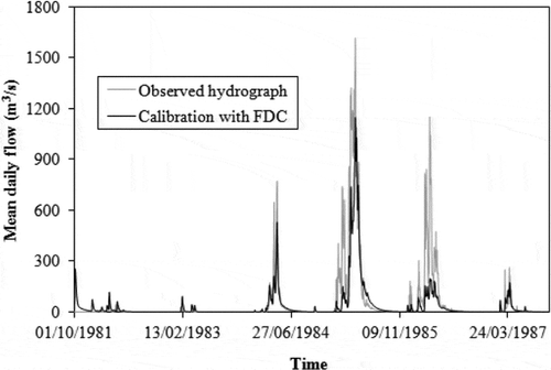
The relatively poorer indices for hydrograph simulation were due largely to the inability of the Rio Grande model to reproduce adequately the observed peak flows, which was noticed in all simulations for the Ceará watersheds, where K index values were always less than 1. This inability to adequately reproduce peak flows is attributed to the changes made in the model structure. In fact, the need to adapt the model structure to accommodate intermittent and ephemeral streams might have caused a considerable loss of water that would eventually sum up to the total runoff.

Further analyses from the observed values of the Nash-Sutcliffe efficiency criterion (E_s) do not seem appropriate, since this index gives relatively greater weight to peak flows. Although the E_s values pointed to good quality of calibration, visual analysis showed that the results were clearly not satisfactory, as exemplified by Fig. 9, which depicts the simulated and observed hydrographs for Fazenda Boa Esperança station (34750000).

Fig. 9 Comparison between the hydrograph obtained by calibration with the FDC and the observed hydrograph at Fazenda Boa Esperança station for the period 1 October 1981–30 September 1987.

8 DISCUSSION AND CONCLUSIONS

The main objective of this paper was to develop a methodology for regionalization of FDCs that is equally applicable to perennial, intermittent and ephemeral streams. For application of the methodology, the extended Burr XII distribution function was used. This distribution proved to be very flexible, satisfactorily reproducing the extremes of FDCs, although it showed a tendency to underestimate streamflow, especially in the low-flow portions of the duration curves.

Regional models identified for the perennial streams in Minas Gerais State showed satisfactory results. Even with the loss of information resulting from the removal of one station in the cross-validation procedure, the JKMs were able to reproduce with reasonable accuracy the empirical FDCs at all stations.

However, for the intermittent streams in Ceará State the results were not too good. The influence of parameter τ on the simulated flows is very strong, and there is a very large increase in the errors calculated when modelled rather than observed values of τ are used. The cross-validation procedure showed that the methodology is not robust or reliable when τ estimates are employed to calculate the FDCs. However, when the performance indices were recalculated taking into account the observed values of the τ parameter, a significant reduction in errors was observed, giving an overall performance close to that observed in the perennial watersheds in Minas Gerais state. This highlights the need to improve the regional procedures for estimating τ. In this regard, we suggest including other hydrogeological variables, more representative or more closely associated with the variation of τ, in the regression equations in order to explain more precisely the streamflow regime in these watersheds. Furthermore, the use of alternative techniques of regression, such as GLS (generalized least squares) or polynomial, can bring significant improvements to the estimates of the “cease-to-flow” parameter.

In addition to the regional models, the FDCs modelled with the extended Burr XII distribution function were used for indirect calibration of the Rio Grande rainfall–runoff model.

For the perennial streams in Minas Gerais State, a comparative assessment of the quality of calibration with FDCs and median ADFCs was performed; calibration with median AFDCs showed better performance. It was also found that simulated hydrographs resulting from calibration with FDCs reproduced the flow recession periods more adequately, while the hydrographs derived from calibration with median AFDCs reproduced the flow peaks more adequately. However, these are preliminary results and we recommend further investigation to achieve more definitive conclusions. New methods for uncertainty analysis, such as those proposed by Serinaldi (2011), can be used to this end.

For the intermittent streams in the State of Ceará, the Rio Grande model structure had to be adapted in order to simulate the no-flow condition. This adaptation, based on the greater withdrawal of water from sub-surface flow and baseflow, allowed the simulation of very low flow values. However, under this model structure, peak flows were not adequately reproduced and simulated runoff volumes were always less than the observed ones.

Acknowledgements

The authors also wish to thank reviewers A. Castellarin and F. Serinaldi for their valuable comments and suggestions.

Funding

The authors wish to thank the agencies FAPEMIG (scholarship for Veber Costa and grant PPM-00158-09) and CNPq (grant 301133/2009-3) for their financial support to this research.

References

- Burr, I.W., 1942. Cumulative frequency functions. Annals of Mathematical Statistics, 13 (2), 215–232.
- Castellarin, A., Camorani, G., and Brath, A., 2007. Predicting annual and long-term flow-duration curves in ungauged basins. Advances in Water Resources, 30 (4), 937–953.
- Castellarin, A., et al., 2004. Regional flow-duration curves: reliability for ungauged sites. Advances in Water Resources, 27, 953–965.
- Cole, R.A.J., Johnston, H.T., and Robinson, D.J., 2003. The use of flow duration curves as a data quality tool. Hydrological Sciences Journal, 48 (6), 939–951.
- Colischonn, W., et al., 2007. The MGB-IPH model for large scale rainfall–runoff modeling. Hydrological Sciences Journal, 52 (5), 878–895.
- Crocker, K., et al., 2003. Flow duration curve estimation in ephemeral catchments in Portugal. Hydrological Sciences Journal, 48 (3), 427–439.
- De Boer, D., 1992. Constraints on spatial transference of rainfall–runoff relationships in semiarid basins drained by ephemeral streams. Hydrological Sciences Journal, 37 (5), 491–504.
- Haan, C.T. 1977. Statistical methods in hydrology. 2nd ed. Ames: The Iowa State University Press.
- Hughes, D.A., 1995. Monthly rainfall–runoff models applied to arid and semiarid catchments for water resources estimation purposes. Hydrological Sciences Journal, 40 (6), 751–769.
- Hughes, D.A. and Smakhtin, V.Y., 1996. Daily flow data time series patching or extension: a spatial interpolation based on flow duration curves. Hydrological Sciences Journal, 41 (6), 851–871.
- Hydrologic Engineering Center, 1981. HEC-1 flood hydrograph package—reference manual. Davis, CA: US Army Corps of Engineers.
- Liu, J. and Han, D., 2010. Indices for calibration data selection of the rainfall–runoff model. Water Resources Research, 46, W04512. doi:10.1029/2009WR008668
- Mohamoud, Y.M., 2008. Prediction of daily flow duration curves and streamflow for ungauged catchments using regional flow duration curves. Hydrological Sciences Journal, 53 (4), 706–724.
- Nadarajah, S. and Kotz, S., 2006. On the extended Burr XII distribution. Hydrological Sciences Journal, 51 (6), 1203–1204.
- Pilgrim, D.H., Chapman, T.G., and Doran, D.G., 1988. Problems of rainfall–runoff modelling in arid and semiarid regions. Hydrological Sciences Journal, 33 (4), 379–400.
- Pinheiro, V.B. and Naghettini, M., 2010. Calibração de um modelo chuva-vazão em bacias sem monitoramento fluviométrico a partir de curvas de permanência sintéticas. Revista Brasileira de Recursos Hídricos, 15 (2), 143–156.
- Ponce, V.M. 1989. Engineering hydrology—principles and practices. Englewood Cliffs, NJ: Prentice Hall.
- Prafulla, P., Yilmaz, K.K., and Gupta, H.V., 2012. Multiple-criteria calibration of a distributed watershed model using spatial regularization and response signatures. Journal of Hydrology, 418, 49–60. doi:10.1016/j.jhydrol.2008.12.004
- Rianna, M., Russo, F., and Napolitano, F., 2011. Stochastic index model for intermittent regimes: from preliminary analysis to regionalization. Natural Hazards and Earth System Sciences, 11, 1189–1203. doi:10.5194/nhess-11-1189-2011
- Serinaldi, F., 2011. Analytical confidence intervals for index flow duration curves. Water Resources Research, 42 (7), W02542.
- Shao, Q., et al., 2004. Models for extremes using the extended three-parameter Burr XII system with application to flood frequency analysis. Hydrological Sciences Journal, 49, 685–700.
- Shao, Q., et al., 2009. A new method for modelling flow duration curves and predicting streamflow regimes under altered land-use conditions. Hydrological Sciences Journal, 54, 606–622.
- Vogel, R.M., 2006. Regional calibration of watershed models. In: V.P. Singh and D.K. Frevert, eds. Watershed models. 1st ed. Boca Raton, FL: CRC Press, 47–74.
- Vogel, R.M. and Fennessey, N.M., 1994. Flow duration curves I: new interpretation and confidence intervals. Journal of Water Resources Planning and Management, 120 (4), 485–504.
- Westerberg, I.K., et al., 2011. Calibration of hydrological models using flow-duration curves. Hydrology and Earth System Sciences, 15, 2205–2227. doi:10.5194/hess-15-2205–2011
- Yu, P.S. and Yang, T.C., 2000. Using synthetic flow duration curves for rainfall–runoff model calibration at ungauged sites. Hydrological Process, 14 (1), 117–133.
- Zhao, R.J., et al., 1980. The Xinanjiang Model. Hydro. Forecasting Proceedings of. Oxford Symposium, IAHS Publication No. 129. Wallingford: International Association of Hydrological Sciences, 351–356.