Groundwater-level forecasting under climate change scenarios using an artificial neural network trained with particle swarm optimization

Abstract

Artificial neural networks (ANNs) have recently been used to predict the hydraulic head in well locations. In the present work, the particle swarm optimization (PSO) algorithm was used to train a feed-forward multi-layer ANN for the simulation of hydraulic head change at an observation well in the region of Agia, Chania, Greece. Three variants of the PSO algorithm were considered, the classic one with inertia weight improvement, PSO with time varying acceleration coefficients (PSO-TVAC) and global best PSO (GLBest-PSO). The best performance was achieved by GLBest-PSO when implemented using field data from the region of interest, providing improved training results compared to the back-propagation training algorithm. The trained ANN was subsequently used for mid-term prediction of the hydraulic head, as well as for the study of three climate change scenarios. Data time series were created using a stochastic weather generator, and the scenarios were examined for the period 2010–2020.

Editor Z.W. Kundzewicz; Associate editor L. See

Citation Tapoglou, E., Trichakis, I.C., Dokou, Z., Nikolos, I.K., and Karatzas, G.P., 2014. Groundwater-level forecasting under climate change scenarios using an artificial neural network trained with particle swarm optimization. Hydrological Sciences Journal, 59(6), 1225–1239. http://dx.doi.org/10.1080/02626667.2013.838005

Résumé

Les réseaux de neurones artificiels (RNA) ont récemment été utilisés pour prévoir la charge hydraulique dans des puits. Dans le présent travail, l’algorithme d’optimisation par essaim de particules (OEP) a été utilisé pour former un RNA multicouche à réglage aval pour la simulation du changement de charge hydraulique dans un puits d’observation de la région d’Agia (Chania, Grèce). Trois variantes de l’algorithme OEP ont été considérées, l’une classique avec amélioration de la masse inertielle, OEP avec coefficients d’accélaration variant au cours du temps (PSO-TVAC) et OEP optimum global et local (GLBest-PSO). La meilleure performance a été obtenue par GLBest-PSO lorsqu’il est implémenté en utilisant des données de terrain de la région étudiée, qui améliorent les résultats de l’algorithme d’apprentissage par rétropropagation. Le RNA formé a ensuite été utilisé pour la prévision à moyen terme de la charge hydraulique ainsi que pour l’étude de trois scénarios de changement climatique. Les séries chronologiques de données ont été créés en utilisant un générateur stochastique de temps, et les scénarios ont été examinés pour la période 2010–2020.

Key words:

• artificial neural networks
• particle swarm optimization
• hydraulic head simulation

Mots clefs:

• réseaux de neurones artificiels
• optimisation par essaim de particules
• simulation de charge hydraulique

1 INTRODUCTION

The models currently used in hydrology for hydraulic head prediction fall into three categories: models based on geomorphology, physically based models and empirical models. Models belonging to the first category can accurately represent the structure of the hydrological system, but require various assumptions concerning the linearity of the system (Gupta and Waymire 1983). Physically based models use mathematical equations that describe the system under consideration; they show the best performance when data on the physical characteristics of the system are available, which usually are not easily accessible. Physically based models have found various applications, including flow modelling (Arnold et al. 2000, Hoffmann et al. 2006) and mass transport (Moon and Song 1997, Dokou and Pinder 2011). Artificial neural networks (ANNs) belong to the category of empirical models, which treat the system as a black box, and their purpose is to find a relationship between input and output data without using any physical data such as hydraulic conductivity and porosity (ASCE 2000).

Artificial neural networks provide an alternative to conventional numerical modelling techniques that are often limited by strict assumptions of normality, linearity and variable independence. They can be used to extract patterns and detect trends from complicated or imprecise data (Haykin 1999). Furthermore, ANNs are widely used in hydrology, for both surface water and groundwater, owing to their capacity to describe nonlinear relationships (Rogers and Dowla 1994, Hsu et al. 1995, Gupta et al. 1997, Rajurkar et al. 2004, Trichakis et al. 2011b). A comprehensive review of ANN applications in hydrology has been presented by Maier and Dandy (2000). Various researchers (Lin and Chen 2006, Samani et al. 2007) used ANNs to identify the parameters of an aquifer and examined the efficiency of networks using multi-layer perceptron ANNs and radial basis function networks. Such models have been successfully used to predict salinity (Maier and Dandy 1996), and to simulate river systems (Maier et al. 2010, Abrahart et al. 2012) and rainfall–runoff processes (Lin and Chen 2008). Several applications of ANNs have focused on the prediction of water level in wells using different input parameters, such as temperature, rainfall and water level in neighbouring wells (Coppola et al. 2005, Lallahem et al. 2005, Nayak et al. 2006). ANNs have also been applied for the prediction of the hydraulic head in wells located in karstic aquifers (Trichakis et al. 2009, 2011a).

Although back-propagation has been used extensively for ANN training, some disadvantages, such as slow training convergence and easy entrapment in a local minimum, are often encountered in the use of this method (Yao 1993, Rojas 1996, Haykin 1999). Alternative optimization methodologies have been applied for ANN training such as conjugate gradient methodology (Towsey et al. 1995), genetic algorithms (GAs) (Rogers et al. 1995) and differential evolution (DE; Trichakis et al. 2009).

Particle swarm optimization (PSO) was developed by Eberhart and Kennedy (1995) as an alternative to GAs and DE algorithms, inspired by the social behaviour of bird flocks and is one of the recent algorithms in the category of evolutionary algorithms. It has been used in various applications and has proven to be an efficient and effective heuristic optimization method, successfully used for ANN training (Chau 2006, Kiranyaz et al. 2009, Akkar 2010). However, PSO has found only limited application in the field of groundwater management. Wegley et al. (2000) used this algorithm to optimize the pumping rate in a water distribution system, while it was also used by Dokou and Karatzas (2013) to optimize the recovery of free-phase light non-aqueous phase liquid (LNAPL). In another study (Gaur et al. 2011), PSO was used to minimize the energy consumption for pumping water, while maintaining an acceptable water level and pressure in storage tanks.

The objective of this study was to examine the use of PSO for training a feed-forward, multi-layer ANN, which simulates the hydraulic head change in an observation well in the area of Agia in Crete, Greece, using the hydraulic head of the previous day, the temperature in the region and the precipitation on the previous day from two meteorological stations. Three variants of the PSO algorithm were utilized and compared with respect to the training and testing errors. The trained ANN was then used for mid-term hydraulic head prediction and for long term prediction using different climate change scenarios.

2 AREA OF STUDY

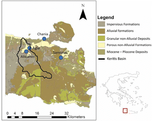
The study area is located in the prefecture of Chania in the region of Agia in Greece (Fig. 1). The area is part of the Keritis basin and has a total area of approximately 30 km². It is the primary water supplier for the city of Chania; so, its significance is high.

Fig. 1 Map showing location of the study area.

The hydrogeological characteristics and geological formations of the study fall into five categories, which include: porous Miocene and Pliocene, porous alluvial and non-alluvial formations, granular non-alluvial deposits and impervious formations, generally with medium to low permeability.

The available data for the study area consist of time series of daily rainfall measurements from two meteorological stations, daily temperature from one station and hydraulic head in the observation well on a daily time-step. The first meteorological station (S1) is located in the Alikianos area and the available rainfall data from this station cover the period between 1 July 2007 and 29 May 2009. The second station (S2) is located in the Samonas area and its data cover the period between 3 July 2007 and 31 May 2009. The available measurements for hydraulic head and temperature correspond to the period between 4 April 2005 and 12 May 2009. The time period selected for the study, providing continuous daily time series for all parameters, spans from 3 July 2007 to 12 May 2009, corresponding to 678 days.

3 ADOPTED METHODOLOGY

3.1 The artificial neural network (ANN)

Artificial neural networks were initially inspired by the structure and functional aspects of biological neural networks, and were originally suggested as mathematical models to simulate human brain function (Haykin 1999). The feed-forward neural network was the first type of ANN, where information moves in only one direction: forward. The processing of information is done at different layers, the corresponding nodes being separated into three categories—input nodes, output nodes and hidden nodes. Input nodes do not perform calculations, while output and hidden nodes are computational nodes. The computational nodes initially multiply the input (x_i) with the corresponding synaptic weight (w_i). The sum of the products of the weights is introduced as an argument to the activation function, and the resulting value is the output value of the node for the current inputs and the weights of a given iteration. This value is then either fed to the next hidden layer or the output of a neural network (ASCE 2000).

In this study, a feed-forward neural network is used to simulate the hydrological equilibrium, described by

(1)

where ΔS is the change in the aquifer storage, I is the inflow of the basin, O is the outflow of the basin, P is the precipitation, EPT is the evapotranspiration and Q is the pumping/recharge rate.

The input parameters of the ANN are directly related to the hydrological equilibrium. Since there are no surface streams in the study area, the surface inflow I and outflow O terms in equation (1) are omitted. Precipitation is a direct input to the ANN model, as measurements from the two meteorological stations in the area, while evapotranspiration is taken into account indirectly, through temperature measurements. Pumping activity data were not available in this region; so, it was assumed that the pumping is constant; therefore, the effect of this parameter will be incorporated in the ANN’s synaptic weights.

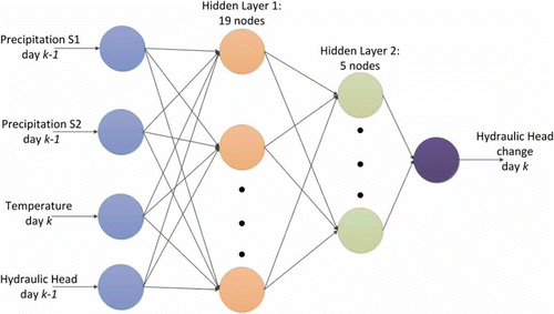
The ANN, used to predict the hydraulic head change on day , has an input layer, which consists of four nodes, namely, temperature, rainfall at meteorological stations S1 and S2 and hydraulic head in the well on day k − 1 (Fig. 2). Note that the input parameters do not include aquifer characteristics such as porosity and hydraulic conductivity. The effect of these parameters will be incorporated in the values of the synaptic weights, thus avoiding the assumption that the aquifer consists of a homogenous medium.

Fig. 2 ΑΝΝ used in this study.

The architecture of a back-propagation ANN developed and used by others in the past (Nikolos 2004, Nikolos et al. 2008, Trichakis et al. 2009) was optimized for the Agia region by Moutzouris (2010). This was achieved by testing various combinations of number of nodes, from one to 20, in each of two hidden layers. The final optimized network architecture consisted of two hidden layers, the first with 19 nodes and the second with five nodes. This configuration is used henceforth as the optimal one for this study area. The output layer consists of a single node, which corresponds to the hydraulic head change on day k, dh_k = h_k – h_k-1, where h_k denotes the hydraulic head on day k. Note that the rainfall at the stations on day k – 1 is considered as the input. This is due to the fact that the optimal time lag between rainfall and the change in hydraulic head is equal to one day for both meteorological stations (Moutzouris 2010). The time lag is the time it takes for the rain to penetrate the soil and reach the aquifer. The correlation coefficient was used in order to define the time lag between precipitation and hydraulic head change.

(2)

where a, b are the values and , the average values of time series A (rainfall) and B (hydraulic head), respectively. Different time lags from 0 to 20 days were tested, and the lag with the highest correlation coefficient was chosen. This procedure was carried out for both weather stations.

The hydraulic head change per time step (day) is used as output, instead of the hydraulic head itself. This is because of the high correlation between the input and output hydraulic head values; this can be as high as 0.998. As a result, the ANN will be highly biased and will tend to underestimate the other input parameters (Trichakis et al. 2009). This means synaptic weights for the hydraulic head input are increased, and for the rest of the input parameters they are decreased.

After the collection of field data, the ANN, defined by Moutzouris (2010), was modified in order to be able to use the PSO algorithm as a training algorithm, instead of back-propagation. The original ANN (back-propagation training method, optimized architecture) is used here as a means to evaluate the efficiency of the newly formulated network (PSO) by comparing their results on the same data set. For network training, the first 80% of the available data are used, while the remaining 20% are used for the evaluation of the trained network. The training and testing errors were calculated using the least mean squared error, between the actual data and the output of the model, as proposed for ANNs, due to its close relation to the back-propagation algorithm (delta rule) (Kröse and van der Smagt 1996).

(3)

where E is the error, N_o is the number of output variables, p is the input pattern, d_o^p is the observed hydraulic head change and y_o^p is the simulated hydraulic head change. Using equation (3), the errors for training (E_train) and testing (E_test) can be calculated using the training and testing data sets, respectively. These errors are indicators of whether the network training was satisfactory or not. The training error reflects the network’s ability to simulate the values which were used for its training. The testing error refers to the error that occurs when values which were not used for training are simulated, and is a measure of the generalization capability of the network. The aim of the training process is to achieve acceptable training and testing errors.

3.2 Particle swarm optimization (PSO)

Particle swarm optimization is a relatively new evolutionary algorithm that can be used to find optimal solutions to numerical and qualitative problems. It was proposed by Eberhart and Kennedy (1995) and was inspired by the social behaviour of animals, such as seen in flocks of birds and shoals of fish. It drew much attention because of its simple computation and rapid convergence features and has been applied to many optimization problems (Wegley et al. 2000, Akkar 2010, Jiang et al. 2010, Afshar 2012).

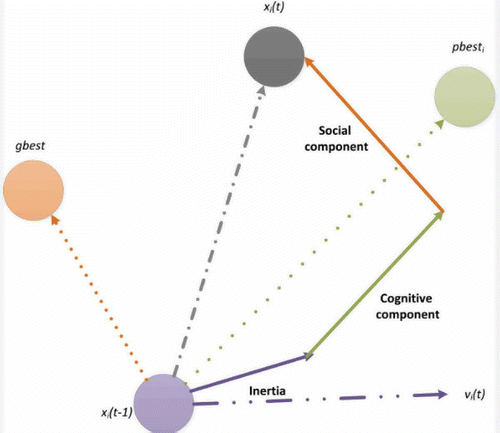
The swarm consists of particles which move in the space defined by the problem. Each particle i represents a candidate solution and is defined by its position vector (x_i) and velocity vector (v_i), where the position vector represents the design variables (parameters) of the problem (Arumugam et al. 2008). In every iteration t of the algorithm, each particle i updates its velocity vector v_i(t) by taking into account its velocity in the (t – 1) iteration v_i(t – 1), its best position pbest_i, and the best position of the swarm, gbest, according to equation (4). The personal best, pbest_i, for particle i is the position where the particle has the best encountered result for the objective function and is used in the calculation of the cognitive component of the velocity update. The global best, gbest, is the best encountered particle position in the swarm. It is used to calculate the social component of the velocity update. In the first version of PSO, the velocity update for iteration t is determined by

(4)

where x_i(t) is the position of particle i in iteration t, c₁ and c₂ are constants known as acceleration coefficients and r₁(t), r₂(t) are random values uniformly distributed in [0,1]. The latter are randomly generated at the beginning of each iteration and they are fixed for all particles during that particular iteration.

The new position of each particle is computed as

(5)

The final trajectory of a particle is schematically presented in Fig. 3 (Eberhart and Kennedy 1995).

Fig. 3 Movement of a particle in each iteration.

In each iteration, the particles are attracted to the optimum solution, based on both their own search and the search of the rest of the swarm. The process terminates when the training error is smaller than a pre-determined value, or when the algorithm completes a specific number of iterations (Poli et al. 2007).

Various modifications to the PSO algorithm have been presented in the past (Eberhart et al. 1996, Clerc 1999, Abraham et al. 2008). These changes aim at improving some characteristic of the method, and their suitability depends on the nature of the problem at hand. Three of the most commonly used variants are the standard PSO (Eberhart and Kennedy 1995), PSO with time varying acceleration coefficients (PSO-TVAC) (Ratnaweera et al. 2004) and global best PSO (GLBest-PSO) (Arumugam et al. 2008), where both the inertia weight and the acceleration coefficients change at the same time (Clerc 1999).

3.2.1 Standard PSO

In the original PSO version (Eberhart and Kennedy 1995), there was no way to control the speed of the particles so as not to get far outside the search space. This drawback was addressed by introducing a new parameter, the inertia weight (Shi et al. 1998a), which can control the impact of the velocity of the particle in iteration (t – 1) on iteration t of the algorithm. In standard PSO, the particle velocity vector is updated according to

(6)

where w is the inertia weight.

3.2.2 PSO-TVAC

In this variation, introduced by Ratnaweera et al. (2004), in addition to the inertia weight, the acceleration coefficients vary linearly with time. However, the change is not the same for c₁ and c₂; the value of c₁ decreases with time, while that of c₂ increases. In this way, the autonomous behaviour of each particle is favoured initially, while progressively the influence of the social component of the swarm is increased. Using the term t/t_max, the exploration of the search space is encouraged early in the process, while the exploitation of the optimal solution is encouraged at the end of the process. In order to do so, the term t/t_max is used in equations (7) and (8). The acceleration coefficients c₁ and c₂ are updated according to

(7)

(8)

where c_1max and c_2max are the maximum values of the acceleration coefficients, c_1min and c_2min are the respective minimum values, t_max is the maximum number of iterations and t the number of the current iteration.

3.2.3 GLBest-PSO

In this variant, presented by Arumugam et al. (2008), both the inertia weight and acceleration coefficients are functions of the personal best solution of each particle and the best solution of the swarm. Specifically, the velocity of each particle is computed as

(9)

where w and C are calculated for every particle and iteration using equations (10) and (11).

(10)

(11)

where (pbest_i)_ave is the average of all the personal best values in that particular iteration.

3.3 PSO algorithm description

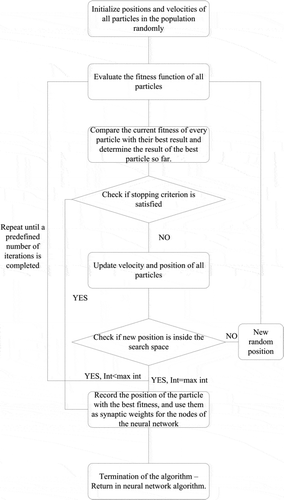
The PSO algorithm is described as follows (Fig. 4). Initially, random positions for all particles in the swarm are generated, ranging from −1 to 1, representing the synaptic weights of the ANNs. In order to initialize the population velocities, random numbers are selected, varying from −0.7 to 0.7. The maximum value that particle positions can have is 2, while the minimum is −2, values which outline the search space of the algorithm.

Fig. 4 Proposed model flowchart for particle optimization algorithm.

Next, the fitness (objective) function—defined here as the training error of the ANN for the current set of synaptic weights—is evaluated for all particles. The current value of the fitness function is evaluated for all particles in order to determine the personal best encountered value for each particle and, in turn, the global best result in the swarm. The positions of the personal and global best results are recorded as well. If the global best is less than a predefined tolerance value, its vector is used as the synaptic weight set for the ANN and the algorithm terminates. If the global best is larger than the tolerance, the position and velocity of all particles are updated and a check is performed to determine whether the new positions lie within the search space. For particles with new positions inside the search space the algorithm is repeated, starting with the evaluation of the fitness function. Otherwise, for particles with new positions outside the search space, new random positions are determined. If the tolerance value is not met after a predefined number of iterations, the algorithm terminates.

The advantages of PSO, compared to other optimization techniques, include simplicity and ease of implementation, and the fact that there are few parameters to adjust, namely number of iterations, swarm size and (depending on the variant) inertia weight and acceleration coefficients. The main advantage of using PSO instead of the back-propagation algorithm to train the ANN is that using the PSO algorithm does not get trapped in local minima and a near-global solution to the problem can be found (Salman et al. 2002, del Valle et al. 2008). However, its parameters can greatly influence the algorithm’s stability and performance, as well as the convergence and simulation results (Shi et al. 1998b).

In this work, PSO was used in order to train the ANN and find the optimal synaptic weights. Specifically, all three variations of the algorithm were tested (the standard algorithm, with the improvements of inertia weight and acceleration coefficients, the PSO-TVAC algorithm and the GLBest-PSO algorithm) in order to compare their performance.

4 RESULTS

All the runs performed in this section were executed on a computer with a 2.53 GHz Core i5 processor. The total number of decision variables was 201, representing the synaptic weights of an ANN with 4 input nodes, 19 and 5 nodes in the first and second hidden layers, respectively, and one output node.

4.1 Choice of appropriate variant

The three different algorithms, the standard algorithm, PSO-TVAC and GLBest-PSO, were tested for a fixed number (10 000) of iterations and for a small swarm size (20). According to Clerc (1999), a swarm that consists of 20–30 particles is sufficient to solve almost all classic test problems. The swarm size chosen to evaluate each algorithm was 20, a comparatively small swarm, but capable of finding a satisfactory solution. The convergence velocity was not a criterion during the selection of the final algorithm variant, since we were focused on minimizing the error irrespective of the time needed.

4.1.1 Standard algorithm

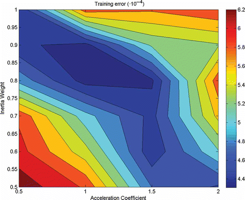
In the standard algorithm, three parameters should be determined: inertia weight w and acceleration coefficients c₁ and c₂. The parameters of the PSO algorithm were optimized simultaneously for different values of the inertia weight, varying from 0.5 to 1 at a step of 0.1, while the acceleration coefficients varied from 0.5 to 2 at a step of 0.5 and for c₁ = c₂. The values obtained from this process are presented in Fig. 5 and they correspond to the training error. Similar behaviour was observed for the testing error. When the acceleration coefficients or the inertia weight takes extreme values, the training error tends to increase. In the case of acceleration coefficients, small values mean that a particle’s movement depends mainly on its previous velocity, while larger values tend to only move particles towards the best solutions found up to that point. Small values of inertia weight are not recommended because, in such a case, the overall velocity of the particle is reduced, narrowing the exploration capabilities. Balancing these two parameters will result in the optimal set, while minimizing the training error.

Fig. 5 Training error surface for different values of inertia weight and acceleration coefficients.

The minimum value of the training error occurs for an inertia weight of 0.8 and acceleration coefficients c₁ = c₂ = 1. At this point, the training error is small because there is a balance between the algorithm’s ability to explore and exploit for the optimal solution. The best result achieved with this algorithm, among the ones presented in Table 1, has a training error of 4.31 × 10^-4 and a testing error of 3.52 × 10^-4.

Table 1 Training and testing errors for various PSO algorithms.

Run no.	Classic PSO		PSO-TVAC		GLBest-PSO
	Etrain(×10^-4)	Etest (×10^-4)	Etrain (×10^-4)	Etest (×10^-4)	Etrain (×10^-4)	Etest (×10^-4)
1	5.64	4.01	5.34	3.76	4.06	3.5
2	5.23	3.66	5.71	4.26	3.94	3.5
3	4.78	3.45	5.67	3.98	3.91	3.62
4	4.76	3.47	5.67	4.14	3.96	3.67
5	4.31	3.52	5.16	3.78	3.85	3.45
6	4.21	3.91	6.01	4.23	4.08	4.08
7	4.23	3.81	5.30	4.40	4.16	3.48
8	4.37	3.99	5.60	3.92	3.95	3.73
9	4.42	3.89	4.96	4.38	4.01	3.62
10	4.15	4.26	5.86	4.23	3.96	3.30
Mean	4.61	3.80	5.53	4.11	3.99	3.60
Execution time (min)	17		20		20

4.1.2 PSO-TVAC algorithm

In this algorithm, the velocity and position of the particles are defined according to equations (6)–(8). According to Ratnaweera et al. (2004), the value of c₁ is initially set at 2.5 and progressively decreases to 0.5, while c₂ is initially set at 0.5 and gradually increases to 2.5. In this way, the algorithm focuses either on the best result of the swarm or on the personal best result of each particle.

4.1.3 GLBest-PSO algorithm

The main advantage of this algorithm is that the parameters are determined based on the position of each particle in relation to the position of the particle with the best result, according to equation (9). The results for the training error, E_train, and the testing error, E_test, for each algorithm under consideration are shown in Table 1 for swarm size of 20 and 10 000 iterations.

The random initialization of particle position and velocity plays an important role in the execution of the algorithm. It causes a fluctuation in the errors for the same number of particles and iterations. Even if initial positions and velocities are held constant, the outcome would not be the same for every execution of the algorithm, since a random parameter is involved in every velocity update. Therefore, 10 test runs were performed for different initial values and the evaluated mean training and testing errors (Table 1) were used for the comparison of the PSO variants. At this point it should also be noted that all three variants required almost the same execution time.

As observed from the results of Table 1, the GLBest-PSO achieved the lowest values for the mean training and testing errors. Specifically, the mean training error for GLBest-PSO was 25.4% and 39.8% smaller than that for Classic PSO and PSO-TVAC, respectively, while the corresponding percentages for the mean testing error were 1.9% and 12.1%. Therefore, GLBest-PSO is the only variant to be considered henceforth. Note that GLBest-PSO exhibits the best performance in most of the runs in Table 1, except for the testing error for runs 3 and 4, where the classic algorithm gives slightly better results.

It should be pointed out that the stochastic procedures used for swarm initialization and repositioning resulted in different final optimal solutions for different runs with the same parameters, a characteristic common for all stochastic optimization methods.

4.2 GLBest-PSO parameter refinement

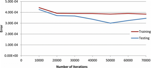
The main tuning parameter of the algorithm is the number of iterations. In order to select the suitable number of iterations for the specific problem, multiple runs were performed using different numbers of iterations, each time varying from 10 000 to 70 000, and for a swarm size equal to 20 (Fig. 6).

Fig. 6 Best training and testing errors vs number of iterations for the GLBest algorithm.

A greater number of iterations resulted in a smaller testing error, until 50 000 iterations were reached, where an increase in the testing error was evident for the larger number of iterations, with the training error remaining almost constant (Fig. 6). The decrease in testing error resulted in an increased generalization capability of the network.

In order to configure the swarm size, the algorithm was executed several times for different swarm sizes of 40–60 particles and for 40 000 iterations. Ten different runs were performed for different initial values and the results obtained are presented in Table 2. An increase in the mean training error and a decrease in the mean testing error were observed when the number of particles in the swarm was increased. That is, the larger the swarm size, the greater the network’s capacity to simulate values for which it has not been trained. The increase in training error can also be expected, because a larger number of particles may result in reduced exploration capability, because multiple near global solutions can be found in different spots in the search space. Therefore, each particle is attracted from these near global solutions towards many different directions, resulting in a decreased ability to reach a local optimum.

Table 2 Training and testing errors for different swarm sizes.

Run no.	Swarm size
	40		50		60
	Etrain (×10^-4)	Etest (×10^-4)	Etrain (×10^-4)	Etest (×10^-4)	Etrain (×10^-4)	Etest (×10^-4)
1	3.68	4.45	3.94	3.74	3.92	3.7
2	3.46	4.49	3.66	4.62	3.95	3.58
3	3.82	4.28	4.1	3.37	4.14	2.85
4	3.71	4.77	3.7	3.95	4.08	3.47
5	3.53	4.58	3.74	4.74	4.26	3.22
6	3.5	4.55	3.87	3.69	3.96	3.43
7	3.43	4.36	3.74	3.93	4.08	3.46
8	3.63	4.72	3.85	4.04	3.92	3.87
9	3.56	4.63	3.87	3.99	3.97	3.44
10	3.93	4.23	4.03	3.68	3.77	3.63
Mean	3.62	4.51	3.85	3.97	4.01	3.46
Execution time (min)	85		100		130

The smallest testing error, equal to 2.847 × 10^-4, was obtained for 60 particles, while the corresponding training error was 4.137 × 10^-4. This run was considered the most appropriate to be used for the simulation of the hydraulic head change in the observation well, despite the fact that there were runs with smaller training errors. The combination of small training error and high testing error is an indication that the network cannot properly simulate values that it has not been trained with (overtraining). In other words, it lacks the generalization ability that is critical if an ANN model is going to be used for testing future scenarios.

The error values for the “best” run were compared to those calculated when using the optimized back-propagation ANN. As shown in Table 3, the training and testing errors are lower in the case where PSO was used for training. Specifically, a 9.3% and 18% improvement was achieved for the training and testing errors, respectively.

Table 3 Comparison of training and testing error for two different training algorithms.

Training method	Etrain	Etest
Back-propagation	4.56 × 10^-4	3.47 × 10^-4
PSO	4.14 × 10^-4	2.85 × 10^-4
Improvement (%)	9.3	18

4.3 Simulation results

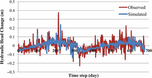
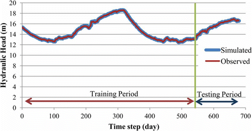
The results for the hydraulic head change obtained by the simulation model (ANN trained with GLBest-PSO with 60 particles and 40 000 iterations) are shown in Fig. 7, along with the observed hydraulic head change.

Fig. 7 Observed and simulated hydraulic head change.

The ANN captured the general trend in hydraulic head change of the natural system, although there are some overestimates and underestimates. Specifically, the magnitude of the difference between observed and simulated values takes a maximum value of 0.35 m, and a minimum of 1.7 × 10^-5 m. The model cannot accurately describe local and transient phenomena that can cause sudden changes in the water level, such as those due to the occasional pumping at nearby wells, or observed at the beginning and/or end of pumping at nearby wells.

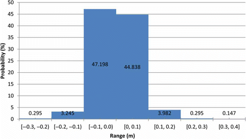
A statistical analysis of the results derived for the hydraulic head change was performed in order to verify the reliability of the simulation. The simulation error values (the difference between observed and simulated data), which ranged from a minimum of – 0.28 m to a maximum of 0.35 m, were divided in seven “bins” of 0.1 m each. The number of days with error belonging to a particular bin was recorded and the probability that the simulation error would fall within a given bin was calculated (Fig. 8). Note that the simulation error is between −0.1 and 0.1 m for over 92% of the days.

Fig. 8 Probability of error magnitude.

For visualization reasons alone the hydraulic head change was then converted a posteriori to hydraulic head (Fig. 9). Specifically, the hydraulic head for day k was obtained by adding the simulated hydraulic head change for day k to the observed hydraulic head for day k – 1.

Fig. 9 Observed and simulated hydraulic head vs time step.

4.4 Mid-term prediction

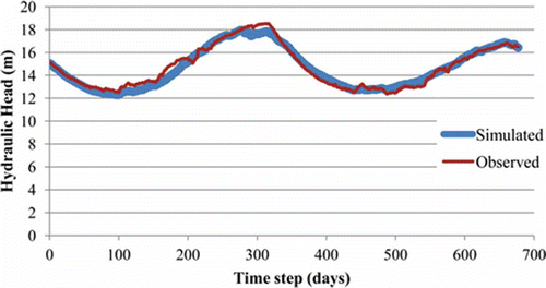
In order to investigate the network’s ability to provide accurate predictions for time periods longer than one day, a prediction period of 678 days was examined. In this case, in order to predict the hydraulic head on day k, the ANN uses the simulated rather than the observed hydraulic head on day k – 1 as input. That is, only the initial observed hydraulic head (day 1) is used for the simulation.

For the mid-term prediction, the trained ANN with the lowest testing error was used (Training method: GLBest-PSO with 40 000 iterations and swarm size 60) and its results together with the observed water level are illustrated in Fig. 10.

Fig. 10 Mid-term prediction.

Generally, the ANN tends to underestimate the hydraulic head. The difference between the simulated and the observed hydraulic heads is, in general, relatively small, with the maximum difference observed at time step 176 equal to −0.97 m. Another significant deviation of the simulated values from the observed values appears between days 286 and 320, the maximum difference being equal to −0.94 m. The accumulated error at the end of the simulation period consisting of almost two hydrological years is equal to only 0.05 m. This value is considered relatively small and insignificant, and therefore implies that the trained network is relatively accurate.

4.5 Climate change scenarios

The trained ANN was subsequently used in order to evaluate the impact of climate change scenarios on the groundwater level of the study area. These scenarios are based on a study by Tsanis et al. (2011), in which a 12% (±25%) reduction in the mean precipitation and a 1.9°C (±0.8°C) increase in the mean temperature are expected in Crete by the end of 2040. This corresponds approximately to a 0.4% (±0.4%) reduction in the mean precipitation per year and a 0.054°C (±0.026°C) increase in the mean temperature per year. Three climate change scenarios were formulated for the period 2010–2020, corresponding to: (a) the average change in precipitation and temperature, (b) the 95% upper and (c) the 95% lower confidence intervals of this prediction.

However, the prediction mentioned above cannot be directly applied to the existing data. This is due to the wet and dry spells that may occur, as well as the fact that the decrease in precipitation refers to the mean precipitation and not to each event separately. Therefore, in order to generate the necessary weather time series for the ANN, a stochastic weather generator, LARS-WG 5.0 (Semenov and Barrow 1997, 2002; http://www.rothamsted.ac.uk/mas-models/larswg.php) was used. The LARS-WG stochastic weather generator can be used for the simulation of weather data at a single site, under both current climate and future climate conditions. There are three steps to the generation of synthetic weather data with LARS-WG: model calibration, in which observed weather data are analysed to determine their statistical characteristics; model validation, in which the statistical characteristics of the observed and synthetic weather data are analysed to determine if there are any statistically significant differences; and, finally, the generation of data from the parameter files derived during calibration (Semenov and Barrow 1997, 2002). For climate change scenarios, daily synthetic data are generated using perturbed statistical characteristics of the observed data.

The LARS-WG is based on the series weather generator described in Racsko et al. (1991). It utilizes semi-empirical distributions for the lengths of wet and dry day series, daily precipitation and daily solar radiation. Precipitation occurrence is modelled as alternate wet and dry series, where a wet day is defined to be a day with non-zero precipitation. For a wet day, the precipitation value is generated from the semi-empirical precipitation distribution for the particular month, independent of the length of the wet series or the amount of precipitation on day k – 1. Daily minimum and maximum temperatures are considered as stochastic processes with daily means and daily standard deviations conditioned on the wet or dry status of the day (Semenov and Barrow 2002).

Three different climate change scenarios that describe average (Scenario 1), severe (Scenario 2, upper 95% confidence interval) and mild (Scenario 3, lower 95% confidence interval) climate change were examined in this work. According to Tsanis et al. (2011), the changes in precipitation and temperature can be further described by the following two equations, for precipitation and temperature, respectively.

(12)

(13)

where P_o is the annual precipitation (mm) in the last known year, T_o is the mean temperature (°C) during the last known year and t is the simulation year.

The last known annual precipitation for station S1 was 739.8 mm year^-1 in 2008, while for station S2 it was 587.4 mm year^-1. The last known mean temperature is 18.4°C. Using equations (12)–(13), the precipitation per year for S1 and S2, as well as the mean annual temperature can be calculated for all years between 2010 and 2020; thus, the percentage of precipitation change was determined. For the temperature the equation was directly applied to the observed data of the last known year and this case constitutes Scenario 1.

Table 4 Rainfall change (%) for Alikianos (S1) and Samonas (S2) weather stations for all three scenarios.

Year	S1			S2
	Scenario 1	Scenario 2	Scenario 3	Scenario 1	Scenario 2	Scenario 3
2010	–0.35	–1.19	0.48	–0.44	–1.28	0.39
2011	–0.71	–2.37	0.96	–0.89	–2.56	0.77
2012	–1.07	–3.57	1.43	–1.35	–3.85	1.15
2013	–1.43	–4.76	1.91	–1.80	–5.13	1.53
2014	–1.79	–5.95	2.38	–2.26	–6.43	1.90
2015	–2.15	–7.15	2.85	–2.73	–7.73	2.27
2016	–2.52	–8.35	3.31	–3.20	–9.03	2.64
2017	–2.89	–9.56	3.78	–3.67	–10.34	3.00
2018	–3.26	–10.76	4.24	–4.15	–11.65	3.35
2019	–3.64	–11.97	4.69	–4.63	–12.96	3.70
2020	–4.02	–13.19	5.15	–5.12	–14.28	4.05

The other two scenarios are based on the 95% confidence interval defined by Tsanis et al. (2011). Specifically, the further percentage reduction in precipitation was applied to the one already calculated in Scenario 1. The change in temperature was directly applied to the last observed data. The final percentages applied to the precipitation for all three climate change scenarios are shown in Table 4, while the temperature increase is provided in Table 5.

Table 5 Temperature increase (°C) for all three scenarios.

Year	Scenario 1	Scenario 2	Scenario 3
2010	0.054	0.090	0.037
2011	0.108	0.144	0.091
2012	0.162	0.198	0.145
2013	0.216	0.252	0.199
2014	0.270	0.306	0.253
2015	0.324	0.360	0.307
2016	0.378	0.414	0.361
2017	0.432	0.468	0.415
2018	0.486	0.522	0.469
2019	0.540	0.576	0.523
2020	0.594	0.630	0.577

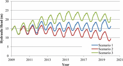
Using the precipitation and temperature time series generated by LARS-WG 5 as input to the ANN that was previously trained by the PSO algorithm, the three climatic scenarios described above were implemented, and the results are summarized in Fig. 11.

Fig. 11 Climate change scenarios.

The hydraulic head exhibits a periodic behaviour for all the scenarios studied. In Scenario 1, there is no particular increase or decrease of the hydraulic head between years, with the mean, maximum and minimum values slightly deviating from the last observed values, as can be seen in Table 6. The average hydraulic head change in this case is positive, but smaller than the current one. However, it must be noted that the current condition refers to the 2 years for which real observations are available (2008–2009), while the data used for the statistical analysis of the scenarios correspond to the period 2010–2020 (synthetic observations created using the weather generator). This is also the reason why the maximum hydraulic head is larger in Scenario 1 compared to the current condition, which only appears once in the study period and does not depict the general tendency of the system. According to this scenario, drought problems are not expected if the same management plan remains in the region.

Table 6 Summary of climate change effect on hydraulic head.

	Hydraulic head (m)
	Mean	Maximum	Minimum	Average change
2008–2009	15.1	18.6	12.46	1.77 × 10^-3
Scenario 1	15.73	19.9	11.7	6.39 × 10^-4
Scenario 2	13	16.8	8.1	–1.06 × 10^-3
Scenario 3	19.5	24.5	11.8	1.88 × 10^-3

Scenario 2 was the least favourable, since it refers to a 13.2% decrease in precipitation at S1 and 14.3% at S2 until the end of 2040. While there is still a periodic behaviour in the hydraulic head data, in this case, particularly between the years 2016–2020, the decrease in the simulated values is significant. In this case minimum, maximum and mean values of the hydraulic head are much smaller than those for Scenario 1 and the current condition. The average hydraulic head change is negative, which means that the area would be losing water and there is an increased possibility of drought problems in the future.

In Scenario 3, the hydraulic head in the well increases with time. This scenario is particularly advantageous, as it forecasts a 5.1% increase in precipitation at S1, and 4% at S2, while there is only a small increase in temperature. In particular, for the period 2012–2020, the increase in the hydraulic head is perceptible compared to the initial hydraulic head, while mean and maximum values are higher than the current ones. Similar to the maximum head in Scenario 1, the minimum value does not behave as expected, but it only refers to a single event. The average hydraulic head change in this case is positive and higher that the current value.

From Fig. 11 it can also be observed that, at the beginning of the prediction period, the hydraulic head was approximately the same for all scenarios. This behaviour continues for scenarios 1 and 2 until 2012, while, for Scenario 3, the deviation from the mean begins as soon as the end of 2011. The deviation in the beginning of the study period is small, due to the fact that the climate change is small and it does not affect the hydraulic head immediately. The only scenario in which the study aquifer is going to face a significant problem, unless the management plan changes, is Scenario 2.

It must also be noted that the results mentioned above may contain errors, which cannot be directly estimated. One source of error could be in the simulation of the ANN, while other potential errors can arise from the statistical data generation from the LARS-WG software, as the existing weather data were not enough to confirm the occurrence of dry or wet spells.

5 CONCLUDING REMARKS

In the present work, PSO was used for training an ANN in order to predict the hydraulic head change in an observation well, using the precipitation from two weather stations, the temperature and the hydraulic head of the well in the Agia region, Chania, Greece as inputs. These parameters are directly connected to the hydraulic equilibrium and the hydraulic head change. More specifically, precipitation can cause a climb in hydraulic head, while increased temperature may lead to increased evapotranspiration and, as a result, reduced hydraulic head levels.

Three different variations of the PSO algorithm were used: the classic algorithm with constant inertia weight and acceleration coefficients; PSO-TVAC, with time-varying acceleration coefficients, which are adjusted in every iteration; and GLBest-PSO, where both inertia weight and acceleration coefficients are time-varying and adjusted at every iteration according to the best personal result and the best result of the swarm. The best training results were obtained with the GLBest-PSO, which achieved smaller training and testing errors when compared to the standard back-propagation algorithm.

The algorithm with the best results, GLBest-PSO, was used to predict the hydraulic head change in an observation well. The ANN was able to accurately describe the general tendency of the natural system, while it could not simulate local and transient phenomena very well, which caused abrupt changes in the hydraulic head, resulting in an underestimation of the observed values in some cases. These changes can be attributed to occasional pumping, or can be observed at the beginning or the end of the pumping period of nearby wells. When the hydraulic head change is converted to hydraulic head, using the observed hydraulic head of the previous day, the deviations of the simulated values from the observed seem comparatively smaller.

The trained ANN was also used for mid-term prediction of the hydraulic head in the observation well. In this case, instead of the measured hydraulic head of each previous day, the simulated hydraulic head is used as an input to the network along with the measured hydraulic head value of the first day of the simulation period. The values obtained by this process were slightly smaller than the observed ones, while in two cases the difference between the observed and the simulated values was higher. However, this error does not accumulate during the simulation period of two hydrological years, and at the end of this period the error is practically negligible.

Finally, three climate change scenarios were studied, depicting small, severe and medium changes in precipitation and temperature in the region. Only the second scenario (i.e. a high decrease in precipitation) resulted in a severe negative effect on the aquifer, while results for the other two scenarios varied from neutral to positive.

REFERENCES

- Abraham, A., Das, S., and Roy, S., 2008. Swarm intelligence algorithms for data clustering. In: O. Maimon and L. Rokach, eds. Soft computing for knowledge discovery and data mining. New York: Springer, 279–313.
- Abrahart, R.J., et al., 2012. Two decades of anarchy? Emerging themes and outstanding challenges for neural network river forecasting. Progress in Physical Geography, 36 (4), 480–513. doi:10.1177/0309133312444943.
- Afshar, M.H., 2012. Large scale reservoir operation by constrained particle swarm optimization algorithms. Journal of Hydro-environment Research, 6 (1), 75–87. doi:10.1016/j.jher.2011.04.003.
- Akkar, H.A.R., 2010. Optimization of artificial neural networks by using swarm intelligent. In: 6th International Conference on Networked Computing (INC). Gyeongju: Institute of Electrical and Electronics Engineers (IEEE), 1–5.
- Arnold, J.G., et al., 2000. Regional estimation of base flow and groundwater recharge in the Upper Mississippi river basin. Journal of Hydrology, 227 (1–4), 21–40. doi:10.1016/S0022-1694(99)00139-0.
- Arumugam, S.M., Rao, M., and Chandramohan, A., 2008. A new and improved version of particle swarm optimization algorithm with global–local best parameters. Knowledge and Information Systems, 16 (3), 331–357. doi:10.1007/s10115-007-0109-z.
- ASCE Task Committee on Application of Artificial Neural Networks in Hydrology, 2000. Artificial neural networks in hydrology. I: preliminary concepts. Journal of Hydrologic Engineering, 5 (2), 115–123. doi:10.1061/(ASCE)1084-0699(2000)5:2(115).
- Chau, K.W., 2006. Particle swarm optimization training algorithm for ANNs in stage prediction of Shing Mun River. Journal of Hydrology, 329 (3–4), 363–367. doi:10.1016/j.jhydrol.2006.02.025.
- Clerc, M., 1999. The swarm and the queen: towards a deterministic and adaptive particle swarm optimization. In: Proceedings of the 1999 congress on evolutionary computation. Washington, DC: Institute of Electrical and Electronics Engineers (IEEE).
- Coppola, E.A., et al., 2005. A neural network model for predicting aquifer water level elevations. Ground Water, 43 (2), 231–241. doi:10.1111/j.1745-6584.2005.0003.x.
- del Valle, Y., et al., 2008. Particle swarm optimization: basic concepts, variants and applications in power systems. IEEE Transactions on Evolutionary Computation, 12 (2), 171–195. doi:10.1109/TEVC.2007.896686.
- Dokou, Z. and Karatzas, G.P., 2013. Multi-objective optimization for free phase LNAPL recovery using evolutionary computation algorithms. Journal of Hydrological Sciences, 58 (3), 671–685.
- Dokou, Z. and Pinder, G.F., 2011. Extension and field application of an integrated DNAPL source identification algorithm that utilizes stochastic modeling and a Kalman filter. Journal of Hydrology, 398 (3–4), 277–291. doi:10.1016/j.jhydrol.2010.12.029.
- Eberhart, R.C., et al., 1996. Computational intelligence PC tools. San Diego, CA: AP Professional.
- Eberhart, R. and Kennedy, J., 1995. A new optimizer using particle swarm theory. Proceedings of the 6th international symposium on micro machine and human science. Nagoya: Institute of Electrical and Electronics Engineers (IEEE), 39–43.
- Gaur, S., Chahar, B.R., and Graillot, D., 2011. Analytic elements method and particle swarm optimization based simulation–optimization model for groundwater management. Journal of Hydrology, 402 (3–4), 217–227. doi:10.1016/j.jhydrol.2011.03.016.
- Gupta, H.V., Kuo-lin, H., and Sorooshian, S., 1997. Superior training of artificial neural networks using weight-space partitioning. In: International conference on neural networks, 9–12 June, Houston, TX, 1919–1923.
- Gupta, V.K. and Waymire, E., 1983. On the formulation of an analytical approach to hydrologic response and similarity at the basin scale. Journal of Hydrology, 65 (1–3), 95–123. doi:10.1016/0022-1694(83)90212-3.
- Haykin, S.S., 1999. Neural networks: a comprehensive foundation. Upper Saddle River, NJ: Prentice Hall.
- Hoffmann, C.C., et al., 2006. Groundwater flow and transport of nutrients through a riparian meadow – field data and modelling. Journal of Hydrology, 331 (1–2), 315–335. doi:10.1016/j.jhydrol.2006.05.019.
- Hsu, K.-L., Gupta, H.V., and Sorooshian, S., 1995. Artificial neural network modeling of the rainfall-runoff process. Water Resources Research, 31 (10), 2517–2530. doi:10.1029/95WR01955.
- Jiang, Y., et al., 2010. Improved particle swarm algorithm for hydrological parameter optimization. Applied Mathematics and Computation, 217 (7), 3207–3215. doi:10.1016/j.amc.2010.08.053.
- Kiranyaz, S., et al., 2009. Evolutionary artificial neural networks by multi-dimensional particle swarm optimization. Neural Networks, 22 (10), 1448–1462. doi:10.1016/j.neunet.2009.05.013.
- Kröse, B. and van der Smagt, P., 1996. An introduction to neural networks. University of Amsterdam.
- Lallahem, S., et al., 2005. On the use of neural networks to evaluate groundwater levels in fractured media. Journal of Hydrology, 307 (1–4), 92–111. doi:10.1016/j.jhydrol.2004.10.005.
- Lin, G.F. and Chen, G.R., 2006. An improved neural network approach to the determination of aquifer parameters. Journal of Hydrology, 316 (1–4), 281–289. doi:10.1016/j.jhydrol.2005.04.023.
- Lin, G.F. and Chen, G.R., 2008. A systematic approach to the input determination for neural network rainfall–runoff models. Hydrological Processes, 22 (14), 2524–2530. doi:10.1002/hyp.6849.
- Maier, H.R. and Dandy, G.C., 1996. The use of artificial neural networks for the prediction of water quality parameters. Water Resources Research, 32 (4), 1013–1022. doi:10.1029/96WR03529.
- Maier, H.R. and Dandy, G.C., 2000. Neural networks for the prediction and forecasting of water resources variables: a review of modelling issues and applications. Environmental Modelling & Software, 15 (1), 101–124. doi:10.1016/S1364-8152(99)00007-9.
- Maier, H.R., et al., 2010. Methods used for the development of neural networks for the prediction of water resource variables in river systems: current status and future directions. Environmental Modelling & Software, 25 (8), 891–909. doi:10.1016/j.envsoft.2010.02.003.
- Moon, H.K. and Song, M.K., 1997. Numerical studies of groundwater flow, grouting and solute transport in jointed rock mass. International Journal of Rock Mechanics and Mining Sciences, 34 (3–4), 206.e201-206.e213.
- Moutzouris, I., 2010. Simulation of water level in an observation well in karstic aquifer using neural networks. Chania: Technical University of Crete.
- Nayak, P., Rao, Y., and Sudheer, K., 2006. Groundwater level forecasting in a shallow aquifer using artificial neural network approach. Water Resources Management, 20 (1), 77–90. doi:10.1007/s11269-006-4007-z.
- Nikolos, I., 2004. Inverse design of aerodynamic shapes using differential evolution coupled with artificial neural network. In: ERCOFTAC conference in design optimization: methods and applications, Athens: European Research Community on Flow, Turbulence and Combustion (ERCOFTAC).
- Nikolos, I.K., et al., 2008. Artificial neural networks as an alternative approach to groundwater numerical modelling and environmental design. Hydrological Processes, 22 (17), 3337–3348. doi:10.1002/hyp.6916.
- Poli, R., Kennedy, J., and Blackwell, T., 2007. Particle swarm optimization. An overview. Swarm Intelligence, 1 (1), 33–57. doi:10.1007/s11721-007-0002-0.
- Racsko, P., Szeidl, L., and Semenov, M., 1991. A serial approach to local stochastic weather models. Ecological Modelling, 57 (1–2), 27–41. doi:10.1016/0304-3800(91)90053-4.
- Rajurkar, M.P., Kothyari, U.C., and Chaube, U.C., 2004. Modeling of the daily rainfall-runoff relationship with artificial neural network. Journal of Hydrology, 285 (1–4), 96–113. doi:10.1016/j.jhydrol.2003.08.011.
- Ratnaweera, A., Halgamuge, S.K., and Watson, H.C., 2004. Self-organizing hierarchical particle swarm optimizer with time-varying acceleration coefficients. IEEE Transactions on Evolutionary Computation, 8 (3), 240–255. doi:10.1109/TEVC.2004.826071.
- Rogers, L.L. and Dowla, F.U., 1994. Optimization of groundwater remediation using artificial neural networks with parallel solute transport modeling. Water Resources Research, 30 (2), 457–481. doi:10.1029/93WR01494.
- Rogers, L.L., Dowla, F.U., and Johnson, V.M., 1995. Optimal field-scale groundwater remediation using neural networks and the genetic algorithm. Environmental Science & Technology, 29 (5), 1145–1155. doi:10.1021/es00005a003.
- Rojas, R., 1996. Neural networks: a systematic introduction. New York: Springer-Verlag.
- Salman, A., Ahmad, I., and Al-Madani, S., 2002. Particle swarm optimization for task assignment problem. Microprocessors and Microsystems, 26 (8), 363–371. doi:10.1016/S0141-9331(02)00053-4.
- Samani, N., Gohari-Moghadam, M., and Safavi, A.A., 2007. A simple neural network model for the determination of aquifer parameters. Journal of Hydrology, 340 (1–2), 1–11. doi:10.1016/j.jhydrol.2007.03.017.
- Semenov, M.A. and Barrow, E.M., 1997. Use of a stochastic weather generator on the development of climate change scenarios. Climatic Change, 35 (4), 397–414. doi:10.1023/A:1005342632279.
- Semenov, M.A. and Barrow, E.M., 2002. LARS – WG: a stochastic weather generator for use in climate impact studies. Hertfordshire: Rothamsted Research.
- Shi, Y. and Eberhart, R., 1998a. A modified particle swarm optimizer. In: IEEE international conference on evolutionary computation. Anchorage, AK: Institute of Electrical and Electronics Engineers (IEEE), 69–73.
- Shi, Y. and Eberhart, R.C., 1998b. Parameter Selection in Particle Swarm Optimization. In: Proceedings of the 7th international conference on evolutionary programming VII, San Diego, CA. New York: Springer-Verlag, 591–600.
- Towsey, M., Alpsan, D., and Sztriha, L., 1995. Training a neural network with conjugate gradient methods. In: Proceedings of IEEE international conference on neural networks. Perth: Institute of Electrical and Electronics Engineers (IEEE), 373–378.
- Trichakis, I., Nikolos, I., and Karatzas, G., 2011a. Artificial Neural Network (ANN) based modeling for karstic groundwater level simulation. Water Resources Management, 25 (4), 1143–1152. doi:10.1007/s11269-010-9628-6.
- Trichakis, I., Nikolos, I., and Karatzas, G.P., 2011b. Comparison of bootstrap confidence intervals for an ANN model of a karstic aquifer response. Hydrological Processes, 25 (18), 2827–2836. doi:10.1002/hyp.8044.
- Trichakis, I.C., Nikolos, I.K., and Karatzas, G.P., 2009. Optimal selection of artificial neural network parameters for the prediction of a karstic aquifer’s response. Hydrological Processes, 23 (20), 2956–2969. doi:10.1002/hyp.7410.
- Tsanis, I., et al., 2011. Severe climate-induced water shortage and extremes in Crete. Climatic Change, 106 (4), 667–677. doi:10.1007/s10584-011-0048-2.
- Wegley, C., Eusuff, M., and Lansey, K., 2000. Determining pump operations using particle swarm optimization. In: Proceedings of the joint conference on water resources engineering and water resources planning and management 2000, Minneapolis, MN: American Society of Civil Engineers (ASCE), 206–206.
- Yao, X., 1993. A review of evolutionary artificial neural networks. International Journal of Intelligent Systems, 8 (4), 539–567. doi:10.1002/int.4550080406.