Modelling radar-rainfall estimation uncertainties using elliptical and Archimedean copulas with different marginal distributions

Abstract

Given that radar-based rainfall has been broadly applied in hydrological studies, quantitative modelling of its uncertainty is critically important, as the error of input rainfall is the main source of error in hydrological modelling. Using an ensemble of rainfall estimates is an elegant solution to characterize the uncertainty of radar-based rainfall and its spatial and temporal variability. This paper has fully formulated an ensemble generator for radar precipitation estimation based on the copula method. Each ensemble member is a probable realization that represents the unknown true rainfall field based on the distribution of radar rainfall (RR) error and its spatial error structure. An uncertainty model consisting of a deterministic component and a random error factor is presented based on the distribution of gauge rainfall conditioned on the radar rainfall (GR|RR). Two kinds of copulas (elliptical and Archimedean copulas) are introduced to generate random errors, which are imposed by the deterministic component. The elliptical copulas (e.g. Gaussian and t-copula) generate the random errors based on the multivariate distribution, typically of decomposition of the error correlation matrix using the LU decomposition algorithm. The Archimedean copulas (e.g. Clayton and Gumbel) utilize the conditional dependence between different radar pixels to obtain random errors. Based on those, a case application is carried out in the Brue catchment located in southwest England. The results show that the simulated uncertainty bands of rainfall encompass most of the reference raingauge measurements with good agreement between the simulated and observed spatial dependences. This indicates that the proposed scheme is a statistically reliable method in ensemble radar rainfall generation and is a useful tool for describing radar rainfall uncertainty.

Editor D. Koutsoyiannis; Associate editor S. Grimaldi

Résumé

Étant donné que les précipitations par radar sont couramment utilisées dans les études hydrologiques, la modélisation quantitative de leur incertitude est très importante, car l’erreur sur les précipitations est la principale source d’erreur dans la modélisation hydrologique. L’utilisation d’un ensemble d’estimations des précipitations est une solution élégante pour caractériser l’incertitude des précipitations par radar et sa variabilité spatiale et temporelle. Cet article propose un générateur d’ensembles pour l’estimation de la précipitation par radar basé sur la méthode des copules. Chaque membre de l’ensemble est une réalisation possible du vrai champ de pluie inconnu, basée sur la distribution des erreurs des précipitations radar (PR) et leur structure spatiale. Nous proposons un modèle d’incertitude constitué d’une composante déterministe et d’un facteur d’erreur aléatoire reposant sur la répartition des précipitations mesurées par des pluviomètres, conditionnée par les précipitations radar (PP|PR). Deux types de copules (à savoir les copules elliptiques et d’Archimède) sont introduites afin de générer des erreurs aléatoires, qui sont imposées par la composante déterministe. Les copules elliptiques (par exemple gaussiennes et t-copules) génèrent des erreurs aléatoires sur la base d’une distribution de plusieurs variables, généralement en décomposant la matrice d’erreur de corrélation par l’algorithme de décomposition LU. Les copules d’Archimède (par exemple Clayton et Gumbel) utilisent la dépendance conditionnelle entre les différents pixels du radar pour obtenir des erreurs aléatoires. C’est sur cette qu’une étude de cas a été réalisée sue le bassin versant de la Brue, situé dans le Sud de l’Angleterre. Les résultats montrent que les marges d’incertitude simulées des précipitations recouvrent la plupart des mesures pluviométriques de référence, avec un bon accord entre les dépendances spatiales simulées et observées. Ceci indique que la méthode statistique proposée est fiable en génération d’ensemble de pluie par radar et se révèle utile pour décrire l’incertitude des radars pluviométriques.

Key words:

• radar-rainfall estimates
• rainfall uncertainties
• copula
• ensemble generation

Mots clefs:

• estimations des précipitations par radar
• incertitudes pluviométriques
• copule
• génération d’ensemble

1 INTRODUCTION

It is widely acknowledged that the uncertainty of real-time hydrological forecasts comes from the model structure, model parameters and the model input (Krajewski et al. 1991, Carpenter 2003, Carpenter and Georgakakos 2004, Smith et al. 2004, Gabellani et al. 2007). Many solutions have been presented to solve the former two factors, such as the generalized likelihood uncertainty estimation (GLUE) (Beven and Binley 1992, Montanari 2005), Bayesian (Krzysztofowicz 1999, Engeland and Gottschalk 2002, Mantovan and Todini 2006, Ajami et al. 2007, Jin et al. 2010) and Markov Chain Monte Carlo (MCMC) (Vrugt et al. 2003, Benke et al. 2008). As modern weather radars are able to provide estimated rainfall with high spatial and temporal resolutions covering a large area, they have been widely used in hydrological applications. However, there are large uncertainties associated with radar-rainfall estimates (Villarini and Krajewski 2010). The uncertainty of model input such as rainfall has been less studied although it is usually more influential than the other two factors. If we can realistically model the uncertainty of the radar rainfall, it should be of great importance in describing the uncertainty of the hydrological model. In this study, modelling of the uncertainties radar rainfall (RR) and generating ensemble rainfall fields are explored which could be directly input to a hydrological model.

There are numerous studies aiming at statistically modelling the error of RR with the help of raingauge information in the literature. Barnston (1991) proposed a so-called error variance separation (EVS) method, which was fully formulated by Ciach and Krajewski (1999a) and Ciach et al. (2003). EVS was able to provide a simple and easy implementation to account for radar data inaccuracy and was applied in many successive studies (Anagnostou et al. 1999, Habib and Krajewski 2002, Chumchean et al. 2003, Habib et al. 2004, 2008, Zhang et al. 2007, Mandapaka et al. 2009, Kirstetter et al. 2010, Bringi et al. 2011, Seo and Krajewski 2011). Ciach et al. (2007) proposed a product-error driven (PED) method to model the RR error by separating the radar uncertainties into deterministic error and random error. There are some decent achievements in this method. First, it is a plain exploratory data analysis and can be easily implemented. Furthermore, the nonparametric characteristics of the method are estimated using a kernel regression approach (Ciach 2003). Raingauge data are used as an approximation of the true rainfall because that is all that is available for the analysis. Finally, this method is within the particular model structure expressing conditional distributions of ‘true’ rainfall as a function of RR. Many applications and improvements have been undertaken based on this model (Habib et al. 2008, Villarini et al. 2008, 2009, Villarini and Krajewski 2009, 2009, 2010, Mandapaka et al. 2010, Habib and Qin 2011). In addition, radar bias including overall bias and conditional bias has been studied and applied in most of the aforementioned error model studies (Smith and Krajewski 1991, Anagnostou et al. 1998, Seo et al. 1999, Borga and Tonelli 2000, Ciach et al. 2000).

Ensemble generation of probable true surface rainfall fields is considered an effective method in modelling the uncertainty of radar rainfall. Krajewski and Georgakakos (1985) generated synthetic radar rainfall by imposing random noise on the known radar-rainfall field. The noise field is determined based on the statistical condition, typically of the mean, variance and correlation to the resultant field. This idea is considered to be the basic conceptual framework in the foregoing studies. Germann et al. (2009) proposed a solution to generate an ensemble of precipitation fields by characterizing the residual errors in RR estimates. It is based on singular value decomposition of the error covariance matrix using the LU decomposition method (Cressie 1992, Goovaerts 1997). However, no strict error model was used in this study. Instead, the RR error was simply regarded as the difference between the radar and gauge rainfall for every time-step, and the variance was computed using the primitive mathematic definition, with the radar intensity as the weight. Villarini et al. (2009) used a similar approach, but with more consideration of the error model. The product-error-driven error model proposed by Ciach et al. (2007) was introduced to compute the deterministic component and build the covariance matrix. In the same way as Germann et al. (2009), this study required the residual error of RR to be Gaussian distributed due to the constraint of the LU decomposition method, which is not always satisfied in all catchments (Anagnostou et al. 1999, Ciach et al. 1999b). In addition, the spatial dependence of residual error was attained using the Pearson correlation coefficient. Due to the limitations and shortcomings of this spatial correlation, more detailed studies are needed. Recently, AghaKouchak et al. (2010a, 2010b) developed an ensemble generation method for remotely-sensed rainfall estimates using copulas. The simulated rainfall fields consisted of the original radar rainfall and uncertainty component multiplied by the radar rainfall, with the assumption that the radar rainfall is proportional to the magnitude of the true rainfall rate (Aghakouchak et al. 2010d, AghaKouchak et al. 2010e). The uncertainty field is generated by a presumed copula. The focus of such research lies on the selection of appropriate copula functions, with little consideration of the marginal distribution of the RR errors.

The main advantage provided by using a copula is that the marginal distribution for each radar pixel can come from different distribution families or different parameters for a family. There is no need to assume a specific distribution, typically in most previous studies, the Gaussian distribution. In this study, uncertainties of RR are fully modelled and ensemble rainfall fields are generated based on the error model. After analysing the statistics of the GR|RR errors, we introduced seven traditional models to fit the GR|RR distribution and optimized the best one. Based on this, we built the multivariate copula to generate the perturbation field. The probable realizations for radar precipitation estimation are obtained by adding the perturbation values to the unperturbed radar rainfall field.

This paper is organized as follows. Section 2 (Data) describes the radar and gauge data used; Section 3 describes the algorithm of generating ensemble rainfall; next we discuss the selection of marginal distribution (Section 4) and the copula functions (Section 5); the outcomes of the simulation and evaluation are presented in Section 6; and, finally, in Section 7, we summarize the key findings and future work.

2 DATA

The Brue catchment in Somerset, southwest England (51.08°N, 2.58°W), was chosen as the experimental catchment for this study (Moore et al. 2000, Roberts et al. 2000). The catchment boundary and terrain elevation are depicted in Fig. 1. The radar and raingauge datasets used were collected from the Hydrology Radar Experiment (HYREX) conducted by the Natural Environment Research Council (NERC) Special Topic Programme. Those data are available through the British Atmospheric Data Centre (BADC, http://badc.nerc.ac.uk/data/hyrex/). The radar used is Wardon Hill radar, located at about 40 km from the centre of the Brue catchment. The radar completes one cycle through four different scan elevations (0.5°, 1.0°, 1.5° and 2.5°) every 5 min, and the lowest one is used here. The spatial resolution of rainfall intensity is 2 km, with 76 × 76 pixels. There are almost 30 pixels covering the Brue catchment and 28 pixels have at least one raingauge (Moore et al. 2000, Wood et al. 2000b) (Fig. 1). The Marshall-Palmer Z–R relationship (Marshall et al. 1955), the standard equation used in the UK (Harrison et al. 2000, Rico-Ramirez and Cluckie 2007), is applied in this study to convert radar reflectivity into rainfall intensity:

(1)

Fig. 1 Map of the raingauge network and the Brue catchment with the terrain elevation as background. The dots represent the raingauge locations and the grid represents the radar pixels. The number in the pixel refers to the index of the corresponding pixel.

where Z and R refer to radar reflectivity and rainfall intensify, respectively. The gauge rainfall is from a dense network of 49 tipping bucket raingauges (TBRs), with 0.2 mm resolution (Bell and Moore 2000, Wood et al. 2000a). The radar and raingauge locations are shown in Fig. 1. The radar and gauge datasets cover the period from October 1993 to April 2000. We accumulate the original data into hourly rainfall in the study. Some typical errors for gauge data, such as timing errors and blockages, are discussed by Bringi et al. (2011). Three typical storm events were chosen for this study. Their start and end times, durations, and accumulated averaged rainfall over the catchment are listed in Table 1. The dataset for the period July–December 1996 is used to compute the correlation coefficients of the generated ensemble.

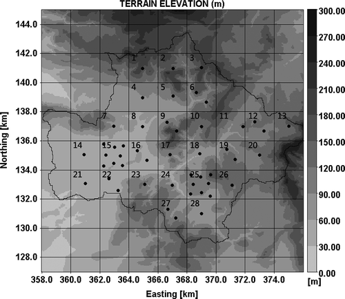
Table 1 Duration and accumulated rainfall for three storm events. Accumulated rainfall is the areally-averaged rainfall in the Brue catchment.

Event	Storm start time	Storm end time	Duration (h)	Accumulated rainfall (mm)
Event A	1995-04-22 00:00	1995-04-23 00:00	24	24.37
Event B	1996-10-14 00:00	1996-10-14 18:00	18	14.32
Event C	1996-11-19 00:00	1996-11-20 06:00	30	34.55

3 ENSEMBLE GENERATOR

Given a radar rainfall estimate, the probable true rainfall can be defined as the sum of the deterministic distortion component and the random component. The ensemble generator for RR estimation produces a number of probable true rainfall outcomes by adding a series of random perturbation fields to the deterministic component of rainfall:

(2)

where is a realistic true areally-averaged pixel-scale rainfall with respect to the radar measurement R_t for ensemble member i and time-step t, h_t(R_t) is the systematic component of radar rainfall conditioned on the given rainfall intensity, and ε_t,i(R_t) represents the corresponding random field, which also depends on the rainfall intensity. The perturbation fields must satisfy two requirements. Primarily, they should yield the marginal distribution of random errors for each radar pixel with reasonable accuracy. In addition, the perturbation fields should maintain the spatial and temporal dependence structure for the whole study area. In this study, we take advantage of a copula to generate a number of perturbation fields.

A copula is defined as a multivariate distribution function whose one-dimensional marginal distributions are uniform on [0,1] (Nelsen 1999). Two kinds of copula are introduced herein, elliptical copulas and Archimedean copulas, due to their special features as explained in Section 5. Suppose ε₁, …, ε_n (n is the number of radar pixels) are random errors of RR with continuous distribution functions F₁, … F_n, then Sklar (1959) proved that there exists a unique copula C such that for all ε = (ε ₁, …, ε_n):

(3)

The main advantage provided by copulas is that the marginal distribution of equation (3) can come from different parametric families. Thus, for example, F₁ might be a Gaussian distribution while F₂ might be from a log-normal family. In the presented scheme, we assume that the distributions of random error for each radar pixel have the same family of distribution, but with different parameters. The detailed assumption as well as the selection of marginal distribution, are discussed in Section 4. The copula is uniquely determined and can be constructed from the marginal functions if the random variables are continuous:

(4)

where u_i is the marginal of random error on [0,1]. For the sake of brevity, a short introduction on copula is presented here. The interested reader can refer to Salvadori et al. (2007) and Nelsen (1999) for the detailed definition and derivation. Using copula, the generation of ensemble RR can be divided into three steps. In the first step, we determine the marginal distribution for each radar pixel. This is achieved by optimizing the empirical uncertainty model for RR estimates using a long-term radar–gauge dataset. It is worth remarking that each radar pixel corresponds to a raingauge in the study area. This is not an essential condition as we only need to build the marginal distribution for those radar pixels having a raingauge. The main parameters and statistical characteristics of the marginal distribution are derived from the distribution of GR|RR (see Section 4). Then the individual marginal distributions are joined together using copula functions. The set of parameters of the copula are obtained through a system of estimating formulas, with each formula being a score function from the marginal distribution (Joe 1997). The score function is the partial derivate of a log-likelihood function. This method is called the Inference Function for Margins (IFM) method (Godambe 1960, 1976, Xu 1996, Joe 1997), which is a special case of the Generalized Method of Moments (GMM). Suppose a copula belongs to a family of copulas indexed by parameter θ and the marginal distributions are indexed by parameter α₁, … α_n, then equation (3) turns out to be:

(5)

From the notations of Sklar’s theorem, the density function of n-dimensional F is written as:

(6)

where f₁, …, f_n are the univariate marginal probability density functions. The foregoing equation implies the following decomposition of the log-likelihood function:

(7)

So the estimation of parameters of a copula function consists of two parts. As we have done the separate optimizations of the marginal univariate likelihoods based on the distribution of GR|RR in the first step, the next problem is to determine the dependence parameter by optimizing the multivariate likelihood function; that is (Genest and Favre 2007):

(8)

Having obtained the parameters of the copula, we can simulate a vector of uniform random variable u (u₁, …u_n) with marginal distributions of U (U₁, … U_n) ( using the copula. The two families of copulas used in this study have different implementation processes in generating random variables. For an elliptical copula, typically of Gaussian copula and t-copula, the related random variables are obtained at the same time based on their multivariate distribution. Take the Gaussian copula for example, we first generate a set of correlated normally distributed variates v (v₁, …v_n) by Choleski’s decompositions (Cressie 1992) of covariance matrix:

(9)

(10)

where µ_v is the mean of the variates, M is the matrix of correlated parameters of the copula function, and ξ is a vector of independent Gaussian random variables with zero mean and unit variance. Then we can transform v (v₁, …v_n) to uniform:

(11)

where Φ is the Gaussian cumulative density function. As a special case, Germann et al. (2009) and Villarini et al. (2009) directly used Choleski’s decompositions to generate a vector of Gaussian distributed random error for RR.

In terms of Archimedean copulas, the uniform random variable u is sampled from the conditioned distributed method. Initially we generate the first random variable u₁ according to its marginal distribution Then the u₂ is attained through generating a variate with uniform distribution U₂ (details can be found in Nelsen 1999). Given U₁ = u₁, u₂ is computed using the quasi-inverse of the conditional distribution function:

(12)

Thus one gets the desired pair (u₁,u₂). The key problem associated with this procedure is solving the conditioned copula. For two variables, the conditional copula is given by (Nelsen 1999):

(13)

As the number of iteration times increases, the maximum theoretical dependence that can be achieved in Archimedean copulas decreases. To reduce the iteration times, the random vector generates from the centre pixel of the study area. Then the values of its four neighbouring pixels (or eight pixels) are obtained based on the aforementioned method. This procedure is repeated until the whole study area is covered. Hence, the multivariate uniform random variables with a given correlation structure are attained. Having these fields, we can obtain the random error with the right marginal distributions by probability integral transform. According to Sklar’s theorem (Sklar 1959), the random error of RR is:

(14)

where F^-1 is the inverse of the continuous distribution functions for random error. In the final step, the random error is superimposed onto the original unperturbed component using equation (2). Thus, we obtain an ensemble of probable rainfall for the whole study area.

4 SELECTION OF MARGINAL DISTRIBUTION

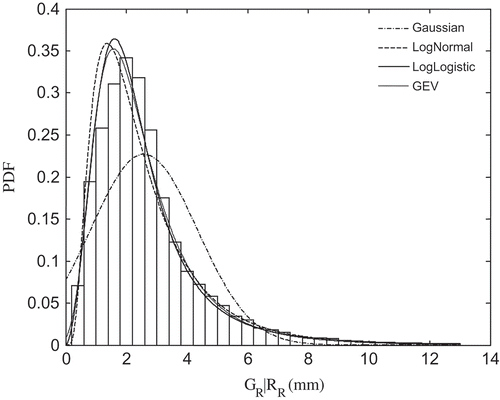
In the literature, the marginal distribution of random error for radar-based estimates is assumed to be either Gaussian or log-normal (Krajewski and Georgakakos 1985, Smith and Krajewski 1993, Anagnostou et al. 1999, Carpenter et al. 2006a, 2006b). In fact, there is an inevitable problem with the Gaussian model due to the fact that the rainfall must be positive. Based on this evidence, we optimize the empirical marginal distribution of random error for RR estimates using a long-term radar–gauge dataset. Presuming the single raingauge rainfall (R_G) can sufficiently represent the true rainfall, where the possible loss under this assumption has been studied in the published literature (Ciach et al. 1999a, Habib et al. 2004, Bringi et al. 2011), the empirical marginal distribution can be fitted using the distribution of GR|RR. We have tested seven distributions which are commonly used in hydrology and meteorology (Gaussian, log-normal, gamma, Weibull, log-logistic, GEV, kappa) and explore the most representative one. The cross-validation is conducted to compare the fit effects of different distributions. The original GR|RR sample is randomly partitioned into a number of subsamples. Among them, a single subsample is retained as the validation data and the remaining subsamples are used to fit the distribution. The Chi-squared test is performed by comparing the observed cumulative distribution function (cdf) of the validation data to the expected one. A series of tests showed that the best model for GR|RR distribution is the generalized extreme value (GEV) model. To illustrate the fitting behaviour of each model, we plotted the probability density function (pdf) for four main distributions, together with the original GR|RR distribution in Fig. 2. Although the Gaussian model is not the most accurate model representing the GR|RR distribution, we still use it here as it is more tractable for the ensemble generator. Based on this evidence, we confine our attention to the GEV and Gaussian models.

Fig. 2 Probability density functions (PDF) of four major models with frequency distributions of the GR|RR. The GR|RR dataset is conditioned on the radar rainfall equals to 3 mm.

The parameters for each model are estimated using the maximum-likelihood estimation method. As the RR error is conditioned on the rainfall intensity, we need to estimate the parameters for each rainfall rate. To get sufficient data for fitting a distribution, we introduce the kernel regression method (Ciach 2003, Ciach et al. 2007). The window size is around 1.8, depending on the different marginal distributions. In other words, the GR|RR dataset is obtained conditioned on a range of RR values centred on a given rainfall rate, rather than conditioned on a single value. To better apply the parameters in the copula estimation, the location and scale parameters of the distribution are fitted using power law functions with a scale coefficient a and exponent coefficient b (see Fig. 3). For example, the location parameter τ can be fitted as:

(15)

Fig. 3 Relationship between the deterministic component (left) and variance (right) of the random error and the rainfall intensities. The scatter points are fitted using power law functions.

Because the shape parameter of the GEV model does not change very much for each rainfall rate, the averaged value is used for the copula estimation. The parameterized results are listed in Table 2. The location parameter is also called a deterministic component in this study. We subtract this deterministic bias when generating the ensemble member for random error, and add it in computing the final ensemble rainfall. As a result, the random error is unbiased.

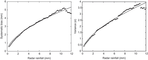
Table 2 Parameters of marginal distribution. Location parameter τ and variance parameter σ are fitted to power law functions; coefficient s refers to the mean of the shape parameters k.

Pixel	Gaussian				GEV
	τ		σ		τ		σ		k
	a	b	a	b	a	b	a	b	s
1	1.82	0.27	1.20	0.32	1.04	0.35	0.65	0.37	0.23
2	1.61	0.35	0.94	0.39	0.97	0.41	0.56	0.47	0.20
3	1.62	0.34	1.17	0.27	1.02	0.35	0.78	0.17	0.25
4	1.59	0.42	1.16	0.38	0.96	0.45	0.59	0.49	0.21
5	1.49	0.37	1.10	0.26	0.87	0.44	0.56	0.42	0.23
6	1.77	0.21	1.31	0.06	1.01	0.32	0.80	0.17	0.18
7	1.33	0.54	0.74	0.65	0.88	0.50	0.56	0.49	0.28
8	1.14	0.66	0.67	0.73	0.87	0.53	0.50	0.58	0.21
9	1.40	0.49	0.65	0.80	0.94	0.39	0.67	0.33	0.38
10	1.89	0.28	1.50	0.28	1.05	0.31	0.78	0.25	0.32
11	1.13	0.71	0.68	0.83	0.99	0.44	0.70	0.37	0.29
12	1.51	0.35	1.51	0.12	0.91	0.34	0.68	0.33	0.20
13	1.55	0.41	1.13	0.55	0.86	0.41	0.56	0.45	0.32
14	1.16	0.63	0.47	1.04	0.88	0.46	0.57	0.47	0.33
15	1.49	0.48	1.24	0.46	0.85	0.49	0.57	0.51	0.26
16	1.35	0.55	0.90	0.53	0.78	0.59	0.55	0.53	0.19
17	1.28	0.64	0.77	0.72	0.94	0.52	0.65	0.48	0.21
18	1.57	0.61	1.76	0.38	1.14	0.43	0.97	0.32	0.35
19	1.32	0.50	0.54	0.82	0.94	0.40	0.67	0.34	0.21
20	1.40	0.42	1.16	0.35	0.89	0.37	0.63	0.36	0.28
21	1.51	0.51	1.10	0.61	0.83	0.49	0.56	0.46	0.42
22	1.33	0.54	0.59	0.80	0.94	0.47	0.67	0.28	0.30
23	1.39	0.46	0.91	0.54	0.81	0.47	0.59	0.43	0.25
24	1.72	0.43	1.47	0.39	1.09	0.36	0.73	0.38	0.27
25	1.64	0.44	1.11	0.44	0.93	0.49	0.64	0.39	0.23
26	1.98	0.21	1.58	0.10	1.08	0.33	0.73	0.32	0.22
27	1.77	0.39	0.95	0.58	1.08	0.39	0.75	0.36	0.23
28	1.52	0.43	0.72	0.69	1.03	0.37	0.62	0.41	0.24

5 COPULA FUNCTIONS AND DEPENDENCE

Two elliptical copulas (Gaussian and t-copula) and two Archimedean copulas (Clayton and Gumbel) are introduced for simulating the ensemble random errors. The elliptical copula is defined as the dependence structure of a correlated elliptical marginal distribution and is attained by standardizing the marginal functions (Mai and Scherer 2012). However, in reality, multivariate elliptical copulas sometimes contain different classes of marginal distributions (not necessarily elliptically distributed), which are also known as meta-elliptical copula (Fang et al. 2002, Abdous et al. 2005, Genest et al. 2007). In this study, we use not only the elliptically marginal distribution (Gaussian model), but also the non-elliptically distributed (GEV) model. The elliptical form of the copula differs from most other copula families such that only an implicit analytical expression is available (Mai and Scherer 2012), and it has a density form f (x^T x). This is the reason why we use the covariance matrix rather than the conditional distribution to obtain the random vector. By far the most commonly used examples of elliptical copulas are the Gaussian copula and t-copula. The multivariate Gaussian copula is determined by a symmetric, positive definite correlation matrix. The t-copula, also known as the Student copula, is defined by two parameters: the aforementioned correlation matrix and the number of degrees of freedom. The bivariate probability density functions for these two copulas are shown in Fig. 4.

Fig. 4 Bivariate copula density functions for (a) Gaussian, (b) t, (c) Clayton and (d) Gumbel copulas. U and V refer to the random variables on [0 1].

The class of Archimedean copulas is a key copula family as they are easy to construct and have good analytical properties. In addition, only one parameter is needed to parameterize Archimedean copulas, which allows the modelling of dependence with arbitrary strength. In fact, Archimedean copulas are not suitable for large-dimensional problems (Joe 1997). The ensemble generation of rainfall using Archimedean copulas is based on the conditional distribution of radar rainfall between two radar pixels. If we produce the ensemble rainfall for each radar pixel one by one, the deviation of the spatial correlation between the first radar pixel and the last one should be vast after 28 (the number of radar pixels) iterations. For this reason, we generate the ensemble rainfall from the centre pixel to the marginal pixel (see Section 3). Thus, only 2–4 iterations are needed. If readers want to apply Archimedean copulas to model the uncertainty of radar rainfall in other study areas, this issue should also be considered. In contrast to the elliptical copula, most common Archimedean copulas allow an explicit formula for the copula function (e.g. Clayton and Gumbel used in this study). The Clayton copula (Clayton 1978, Cook and Johnson 1981, 1986) is a positively-ordered asymmetric copula, exhibiting greater dependence coefficients in the negative tail than in the positive, whereas the Gumbel copula (Gumbel 1960), also known as Gumbel-Hougard copula, has higher positive tail dependence compared to the negative one. The bivariate pdfs for these two copulas are depicted in Fig. 4.

To test the goodness of the presented scheme, the dependence of the generated ensemble variable derived by copulas is compared to the correlation between the original data. There are two methods that measure the dependence: the Pearson correlation coefficient and the rank correlation coefficient. As the Pearson correlation coefficient only measures the linear relationship without anomalous values between the variables, only the rank correlation coefficient is considered in this study. Rank correlation incorporates the information about the dependence between the variables, which is independent of their marginal behaviour. Kendall’s tau correlation coefficient (Kendall 1970) is a typical rank correlation, which takes advantage of concordance to compute the correlation between two variables. For n observations X (x₁, … x_n) and Y (y₁, … y_n), the number that are concordant C and discordant D are denoted:

(16)

(17)

Then Kendall’s coefficient is defined as:

(18)

The challenge for comparing the dependence of copula and Kendall’s correlation is to derive the relationship between them, which varies with copula models. For the Gaussian and t-copulas, the relationship is obtained based on the correlation parameter ρ of the copula (Salvadori et al. 2007):

(19)

There is only one parameter (dependence parameter θ) that exists in Clayton and Gumbel copulas. So the conversion lies in the θ and rank correlation coefficient τ. They are given by (Salvadori et al. 2007):

(20)

(21)

Except for the Gaussian dependence between two variables, the tail dependence (Joe 1997, Schmidt 2002, Melchiori 2003, Aghakouchak et al. 2010c, Salvadori and De Michele 2013) of copulas also play a key role in describing the characteristics of RR. In essence, the so-called tail dependence describes the limiting proportion that one margin exceeds a certain threshold given that the other margin has already exceeded that threshold (see Joe 1997, Aghakouchak et al. 2010c, AghaKouchak et al. 2013, for more critical definitions of tail dependence). The upper tail can give the probability occurrence of positive large values at a joint condition. So modelling the upper tail dependence is of great importance for extreme rainfall. Among the four copulas applied in this study, the upper tail dependence coefficients of Gaussian and Clayton copulas are equal to zero. From this point of view, they are not the preferred method in describing extreme rainfall. The lower and upper tail dependence coefficients of t-copula are equal (Salvadori et al. 2007):

(22)

where t_v denotes the univariate student distribution with v degrees of freedom. The upper tail of a Gumbel copula (Salvadori et al. 2007) is expressed with the dependence parameter as:

(23)

6 RESULTS

As discussed, we used the IFM method to estimate the parameters of copula functions. The parameters of the marginal distribution and dependence are fixed and obtained before the generation of ensemble rainfall. At each time-step, one has a vector of rainfall for 28 radar pixels. Then each marginal distribution is determined according to the relationship between rainfall intensities and parameters. The spatial dependence parameters depend on the spatial location between different radar pixels. Having these parameters, one can generate a vector of random variables, and consequently, transform them based on Sklar’s theorem to get the ensemble rainfall. Figure 5 shows the generated ensemble (500 realizations) using Gaussian and Gumbel copulas with the Gaussian marginal distribution for the three events (Table 3). Corresponding plots (Fig. 6) are presented for the GEV marginal distribution. The solid line represents the gauge rainfall and the shaded area is the simulated rainfall ensembles with the dashed line as the unperturbed fields. As expected, the uncertainty of radar rainfall is proportional to the magnitude of the rainfall intensity. With a few exceptions, the estimated uncertainty bands encompass the raingauge measurements. The differences between the uncertainty bands of different copulas are relatively small. The copula mainly determines the spatial correlation between different radar pixels. There are significant differences between the uncertainty bands for marginal distributions. For example, the dashed line (refers to the deterministic component) is almost in the centre of the uncertainty band for the Gaussian distribution, which cannot be observed for the GEV distribution. We use the theoretical cumulative distribution function (cdf) instead of the observed cdf in generating the vector of random errors because there is not enough data to create a reasonable observed cdf in some cases, especially for extreme rainfall.

Fig. 5 Generated ensemble (500 realizations) using Gaussian (top) and Gumbel (bottom) copulas with the Gaussian marginal distribution for the three events detailed in Table 3.

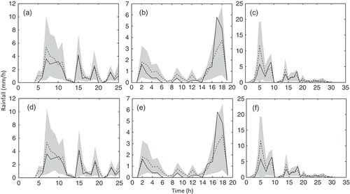
Fig. 6 Generated ensemble (500 realizations) using Gaussian (top) and Gumbel (bottom) copulas with the GEV marginal distribution for the three events detailed in Table 3.

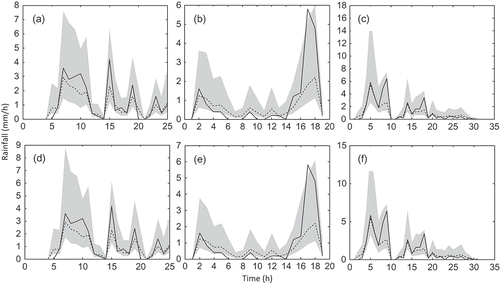
Table 3 Mean absolute error (MAE) of the simulated and observed correlation matrixes for four copulas. Theoretical and tail correlations refer to the simulated correlation coefficient derived by copula dependence parameters and tail dependence parameters, respectively. Generated correlation refers to the spatial correlation coefficient between different radar pixels computed using the generated ensemble rainfall.

	Gaussian	t	Clayton	Gumbel
Theoretical correlation	0.019	0.007	0.067	0.015
Generated correlation	0.093	0.069	0.148	0.105
Tail correlation	-	0.053	-	0.122

To assess the performance of the proposed scheme, we need to test the marginal distribution of rainfall for each radar pixel and dependence between different pixels. As copulas can maintain the marginal characteristics, the spatial dependence is of more concern. The simulated correlation coefficients can be computed in two ways. The first method is to derive the theoretical correlation coefficients using equations (19)–(21), based on the relationship between the dependence parameters of copulas and rank correlation coefficients, which is the so-called theoretical correlation. We can also compute them by the generated ensemble rainfall, which is named the generated correlation. Figure 7 shows the correlation matrices for 28 pixels derived from the copula dependence and observed data. The rank correlation matrices calculated using the observed radar data and gauge data are shown in Fig. 7(a) and (b) respectively. There are two obvious characteristics in the observed radar rainfall estimates (RRE) fields (Fig. 7(a)). Primarily, the maps seem to be divided by a couple of squared zones, and except for the main diagonal line, where the correlation coefficients are equal to one, there are two minor oblique lines with high correlation coefficients. These features are caused by the distances of different pixels. For example, the correlation coefficient between the 7th pixel and 14th pixel is relatively high, as they are close to each other (see Fig. 1). Looking at the correlation matrices derived by different copulas, we can still crudely observe the minor oblique lines, indicating that the copula can maintain the high correlation. The squared zones are not obvious, but can still be observed from the simulated matrices.

Fig. 7 Correlation matrices (for 28 radar pixels) based on original radar rainfall estimates (RRE), raingauge measurement and four copulas, respectively.

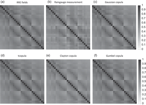
To quantitatively compare the performance of different copulas and marginal distributions, the mean absolute errors (MAEs) of the simulated correlation matrix with respect to the observed correlation matrix are listed in Table 3. Results are given only for the Gaussian marginal distribution, as the marginal distribution has no influence on the dependence behaviour of copulas. As stated earlier, the tail dependence plays a vital role in hydrological applications, and so the performance of the tail dependence generated by the proposed scheme is also investigated. The rank correlations of copulas are calculated based on equations (22)–(23) using the tail dependence parameters of the copulas. Except for the Clayton and Gumbel copulas, the MAEs are less than 0.1 in all cases. The correlations attained by the generated ensemble are generally worse than those of the theoretical ones. This is possible as the realizations are obtained randomly at each time-step (only one member is generated at each time-step) and outline values may contaminate the outcomes. In all cases the t-copula results are better than for any other copulas. Given that the t-copula can also describe the tail dependence of the observed rainfall well, it is the best choice among the considered copulas.

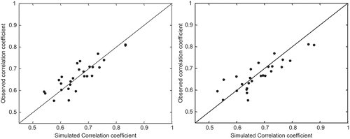
To better illustrate the effects, we plotted the comparison of the simulated and observed correlation coefficients in Figs 8–10. The correlation coefficients are computed between the central pixel of the catchment (Pixel 17) and the other pixels. Figure 8 shows the simulated theoretical correlation and that this proposed method almost accurately simulates the spatial correlation of the observed correlations. In terms of tail dependence (see Fig. 9), there is an obvious overestimation of the simulated fields for the Gumbel copula. The level of overestimation is nearly constant, so it can be regarded as a bias in the process of generating the ensemble. There is also visual agreement between the two correlation coefficients in Fig. 10 for the correlation calculated using the ensemble members. In Fig. 10 the simulation procedure was carried out with a dataset covering the period July 1996 to December 1996. It is apparent that the differences between the simulated and observed correlations do not always decrease with the growth of dataset size.

Fig. 8 Comparison of simulated spatial correlation coefficient between different radar pixels through theoretical equations and observed correlation coefficient for Gaussian (left) and Gumbel (right) copulas for Pixel 17.

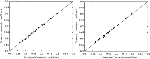
Fig. 9 Comparison of the spatial correlation coefficients between different radar pixels derived from tail dependence and observed correlation coefficients for the t-copula (left) and Gumbel copula (right).

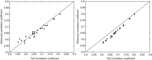
Fig. 10 Comparison of simulated correlation coefficient using generating random variable and observed correlations coefficient for the Gaussian (left) and Gumbel (right) copulas for Pixel 17. The data cover the period between July and December of 1996.

The intergauge rank correlation coefficients of random error are shown in Fig. 11, which illustrates the relationship between the correlation coefficients and lag distances. We fit the scattered points with a three-parameter exponential function:

(24)

Fig. 11 Spatial correlation of the radar rainfall error with a three-parameter exponential model. The left figure refers to correlation of the original observed data, and the right one is that of the generated ensemble.

where Δs is the lag distance, ρ₀ refers to the immediate correlation jump, R₀ is the long correlation radius, and F is the shape coefficients of the parametric model. The fitted coefficients are listed in Table 4. We compare the spatial correlations computed by the generated ensemble rainfall and the original observed data. The good agreement between two fitted curves proves that the proposed method can maintain the spatial dependence between different pixels quite well.

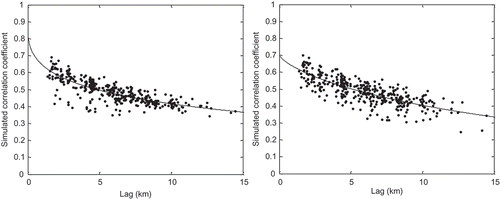
Table 4 Coefficients of the parameterized model for the spatial correlation of the original observed rainfall and generated ensemble rainfall.

Coefficients	Observed	Simulated
ρ0	0.72	0.70
R0	21.16	22.80
F	0.65	0.72

7 SUMMARY AND DISCUSSION

In this paper a fully formulated scheme for ensemble radar rainfall generation based on elliptical and Archimedean copulas is proposed with different marginal distributions. The output ensemble rainfall can maintain the marginal distribution for each radar pixel as well as the spatial dependence across the whole study area. The fact that the simulated uncertainty band of radar rainfall encompasses most of the reference raingauge measurements, and with a good agreement between the simulated and observed spatial dependences, proves the accuracy of the proposed scheme. The key findings can be summarized as follows:

1. The uncertainty model of RR based on the conditional GR|RR distribution can perform well in generating ensemble radar rainfall.

2. The GEV model is the best distribution for representing the marginal distribution of the error of RR in the Brue catchment. The Gaussian model, which is commonly used as an error model, also achieves good performances in the ensemble generation. In addition, the location and scale parameters of both models can be fitted with a power law equation.

3. The case study in the Brue catchment reveals that the Gaussian, t-copula and Clayton copulas simulate the spatial dependence of RR values with slight differences compared with the observed rank correlation coefficients.

4. The tail dependence is of great importance in modelling the extreme rainfall. The copula functions can achieve good performances in simulating upper tail dependence.

It is generally recognized that there are three constraints in generating ensemble radar rainfall, namely the marginal constraints, spatial dependence and temporal dependence. In the course of implementing the presented scheme, we only consider the former two factors. Habib et al. (2008) concluded that the temporal autocorrelation can be neglected as it is close to zero for larger time lags. Despite this, it is commonly agreed that the radar rainfall error does have temporal dependence during short time lags (Ciach et al. 2007, Germann et al. 2009). We believe that temporal dependence can also be incorporated into the proposed scheme. More precisely, we generate the ensemble rainfall from the central pixel (Pixel 17) of the study area for Archimedean copulas in this study (which is also considered as the seed pixel), and then proceed to the whole area based on the spatial conditional distribution of RR. To maintain the temporal consistence, one may generate the ensemble rainfall for the next time from the seed pixel based on the temporal conditional distribution. Then the rainfall values of the other pixels at the next time-step are obtained based on the seed rainfall. This procedure is repeated until the end of the event. It is a simple and practical approach and easily implemented in the real-time hydrological system. However, with the growth of time-steps, the temporal dependence may diverge from the real dependence as the method is based on the conditioned correlation. Besides this approach, autoregressive filtering is also a promising method for recognizing the temporal dependence. The integration of the copula method and a second-order autoregressive model provides a possible solution to describe the spatio-temporal uncertainty of radar-rainfall estimation. This scheme is rooted in imposing the desired temporal structure on the generated ensemble rainfalls which satisfy the marginal and spatial constraints. Exploration of those approaches will be carried out in future work.

REFERENCES

- Abdous, B., Genest, C., and Rémillard, B., 2005. Dependence properties of meta-elliptical distributions. In: Statistical modeling and analysis for complex data problems. New York: Springer, 1–15. doi:10.1007/0-387-24555-3_1
- AghaKouchak, A., Bárdossy, A., and Habib, E., 2010a. Conditional simulation of remotely sensed rainfall data using a non-Gaussian v-transformed copula. Advances in Water Resources, 33 (6), 624–634. doi:10.1016/j.advwatres.2010.02.010
- AghaKouchak, A., Bárdossy, A., and Habib, E., 2010b. Copula‐based uncertainty modelling: application to multisensor precipitation estimates. Hydrological Processes, 24 (15), 2111–2124.
- Aghakouchak, A., Ciach, G., and Habib, E., 2010c. Estimation of tail dependence coefficient in rainfall accumulation fields. Advances in Water Resources, 33 (9), 1142–1149. doi:10.1016/j.advwatres.2010.07.003
- Aghakouchak, A., Habib, E., and Bárdossy, A., 2010d. A comparison of three remotely sensed rainfall ensemble generators. Atmospheric Research, 98 (2–4), 387–399. doi:10.1016/j.atmosres.2010.07.016
- AghaKouchak, A., Habib, E., and Bárdossy, A., 2010e. Modeling radar rainfall estimation uncertainties: random error model. Journal of Hydrologic Engineering, 15 (4), 265–274. doi:10.1061/(ASCE)HE.1943-5584.0000185
- AghaKouchak, A., Sellars, S., and Sorooshian, S., 2013. Methods of tail dependence estimation. In: Extremes in a changing climate. New York: Springer, 163–179. doi:10.1007/978-94-007-4479-0_6
- Ajami, N.K., Duan, Q., and Sorooshian, S., 2007. An integrated hydrologic Bayesian multimodel combination framework: confronting input, parameter, and model structural uncertainty in hydrologic prediction. Water Resources Research, 43 (1).
- Anagnostou, E.N., et al., 1998. Mean-field rainfall bias studies for WSR-88D. Journal of Hydrologic Engineering, 3 (3), 149–159.
- Anagnostou, E.N., Krajewski, W.F., and Smith, J., 1999. Uncertainty quantification of mean-areal radar-rainfall estimates. Journal of Atmospheric and Oceanic Technology, 16 (2), 206–215.
- Barnston, A.G., 1991. An empirical method of estimating raingage and radar rainfall measurement bias and resolution. Journal of Applied Meteorology, 30, 282–296. doi:10.1175/1520-0450(1991)030<0282:AEMOER>2.0.CO;2
- Bell, V. and Moore, R., 2000. The sensitivity of catchment runoff models to rainfall data at different spatial scales. Hydrology and Earth System Sciences Discussions, 4 (4), 653–667. doi:10.5194/hess-4-653-2000
- Benke, K.K., Lowell, K.E., and Hamilton, A.J., 2008. Parameter uncertainty, sensitivity analysis and prediction error in a water-balance hydrological model. Mathematical and Computer Modelling, 47 (11–12), 1134–1149. doi:10.1016/j.mcm.2007.05.017
- Beven, K. and Binley, A., 1992. The future of distributed models: model calibration and uncertainty prediction. Hydrological Processes, 6 (3), 279–298. doi:10.1002/hyp.3360060305
- Borga, M. and Tonelli, F., 2000. Adjustment of range-dependent bias in radar rainfall estimates. Physics and Chemistry of the Earth, Part B: Hydrology, Oceans and Atmosphere, 25 (10–12), 909–914. doi:10.1016/S1464-1909(00)00124-6
- Bringi, V., Rico-Ramirez, M., and Thurai, M., 2011. Rainfall estimation with an operational polarimetric c-band radar in the United Kingdom: comparison with a gauge network and error analysis. Journal of Hydrometeorology, 12 (5), 935–954. doi:10.1175/JHM-D-10-05013.1
- Carpenter, T.M., 2003. A methodology for assessing the utility of distributed model forecast applications in an operational environment. In: Y. Tachikawa, et al. eds. Weather radar information and distributed hydrological modelling. Wallingford: International Association of Hydrological Sciences, IAHS Publ. 282, 85–92. http://iahs.info/uploads/dms/iahs_282_085.pdf [Accessed 29 August 2014].
- Carpenter, T.M. and Georgakakos, K.P., 2004. Impacts of parametric and radar rainfall uncertainty on the ensemble streamflow simulations of a distributed hydrologic model. Journal of Hydrology, 298 (1–4), 202–221.
- Carpenter, T.M. and Georgakakos, K.P., 2006a. Discretization scale dependencies of the ensemble flow range versus catchment area relationship in distributed hydrologic modeling. Journal of Hydrology, 328 (1–2), 242–257. doi:10.1016/j.jhydrol.2005.12.008
- Carpenter, T.M. and Georgakakos, K.P., 2006b. Intercomparison of lumped versus distributed hydrologic model ensemble simulations on operational forecast scales. Journal of Hydrology, 329 (1), 174–185.
- Chumchean, S., Sharma, A., and Seed, A., 2003. Radar rainfall error variance and its impact on radar rainfall calibration. Physics and Chemistry of the Earth, Parts A/B/C, 28 (1–3), 27–39. doi:10.1016/S1474-7065(03)00005-6
- Ciach, G.J., 2003. Local random errors in tipping-bucket rain gauge measurements. Journal of Atmospheric and Oceanic Technology, 20 (5), 752–759. doi:10.1175/1520-0426(2003)20<752:LREITB>2.0.CO;2
- Ciach, G.J., Habib, E., and Krajewski, W.F., 2003. Zero-covariance hypothesis in the error variance separation method of radar rainfall verification. Advances in Water Resources, 26 (5), 573–580.
- Ciach, G.J. and Krajewski, W.F., 1999a. On the estimation of radar rainfall error variance. Advances in Water Resources, 22 (6), 585–595. doi:10.1016/S0309-1708(98)00043-8
- Ciach, G.J. and Krajewski, W.F., 1999b. Radar-rain gauge comparisons under observational uncertainties. Journal of Applied Meteorology, 38 (10), 1519–1525. doi:10.1175/1520-0450(1999)038<1519:RRGCUO>2.0.CO;2
- Ciach, G.J., Krajewski, W.F., and Villarini, G., 2007. Product-error-driven uncertainty model for probabilistic quantitative precipitation estimation with NEXRAD data. Journal of Hydrometeorology, 8 (6), 1325–1347. doi:10.1175/2007JHM814.1
- Ciach, G.J., Morrissey, M.L., and Krajewski, W.F., 2000. Conditional bias in radar rainfall estimation. Journal of Applied Meteorology, 39 (11), 1941–1946. doi:10.1175/1520-0450(2000)039<1941:CBIRRE>2.0.CO;2
- Clayton, D.G., 1978. A model for association in bivariate life tables and its application in epidemiological studies of familial tendency in chronic disease incidence. Biometrika, 65 (1), 141–151.
- Cook, R.D. and Johnson, M.E., 1981. A family of distributions for modelling non-elliptically symmetric multivariate data. Journal of the Royal Statistical Society. Series B (Methodological), 43 (2), 210–218.
- Cook, R.D. and Johnson, M.E., 1986. Generalized Burr-Pareto-logistic distributions with applications to a uranium exploration data set. Technometrics, 28 (2), 123–131.
- Cressie, N., 1992. Statistics for spatial data. Terra Nova, 4 (5), 613–617. doi:10.1111/j.1365-3121.1992.tb00605.x
- Engeland, K. and Gottschalk, L., 2002. Bayesian estimation of parameters in a regional hydrological model. Hydrology and Earth System Sciences Discussions, 6 (5), 883–898.
- Fang, H.-B., Fang, K.-T., and Kotz, S., 2002. The meta-elliptical distributions with given marginals. Journal of Multivariate Analysis, 82 (1), 1–16. doi:10.1006/jmva.2001.2017
- Gabellani, S., et al., 2007. Propagation of uncertainty from rainfall to runoff: a case study with a stochastic rainfall generator. Advances in Water Resources, 30 (10), 2061–2071. doi:10.1016/j.advwatres.2006.11.015
- Genest, C., et al., 2007. Metaelliptical copulas and their use in frequency analysis of multivariate hydrological data. Water Resources Research, 43 (9). doi:10.1029/2006WR005275
- Genest, C. and Favre, A.-C., 2007. Everything you always wanted to know about copula modeling but were afraid to ask. Journal of Hydrologic Engineering, 12 (4), 347–368.
- Germann, U., et al., 2009. REAL—Ensemble radar precipitation estimation for hydrology in a mountainous region. Quarterly Journal of the Royal Meteorological Society, 135 (639), 445–456. doi:10.1002/qj.375
- Godambe, V., 1960. An optimum property of regular maximum likelihood estimation. The Annals of Mathematical Statistics, 31 (4), 1208–1211.
- Godambe, V., 1976. Conditional likelihood and unconditional optimum estimating equations. Biometrika, 63 (2), 277–284.
- Goovaerts, P., 1997. Geostatistics for natural resources evaluation. New York: Oxford University Press on Demand.
- Gumbel, E.J., 1960. Bivariate exponential distributions. Journal of the American Statistical Association, 55 (292), 698–707.
- Habib, E., Aduvala, A.V., and Meselhe, E.A., 2008. Analysis of radar-rainfall error characteristics and implications for streamflow simulation uncertainty. Hydrological Sciences Journal, 53 (3), 568–587. doi:10.1623/hysj.53.3.568
- Habib, E., Ciach, G.J., and Krajewski, W.F., 2004. A method for filtering out raingauge representativeness errors from the verification distributions of radar and raingauge rainfall. Advances in Water Resources, 27 (10), 967–980. doi:10.1016/j.advwatres.2004.08.003
- Habib, E. and Krajewski, W.F., 2002. Uncertainty analysis of the TRMM ground-validation radar-rainfall products: application to the TEFLUN-B field campaign. Journal of Applied Meteorology, 41 (5), 558–572. doi:10.1175/1520-0450(2002)041<0558:UAOTTG>2.0.CO;2
- Habib, E. and Qin, L., 2011. Application of a radar‐rainfall uncertainty model to the NWS multi‐sensor precipitation estimator products. Meteorological Applications, 20 (3), 276–286.
- Harrison, D., Driscoll, S., and Kitchen, M., 2000. Improving precipitation estimates from weather radar using quality control and correction techniques. Meteorological Applications, 7 (2), 135–144. doi:10.1017/S1350482700001468
- Jin, X., et al., 2010. Parameter and modeling uncertainty simulated by GLUE and a formal Bayesian method for a conceptual hydrological model. Journal of Hydrology, 383 (3–4), 147–155. doi:10.1016/j.jhydrol.2009.12.028
- Joe, H., 1997. Multivariate models and dependence concepts. London: Chapman Hall.
- Kendall, M.G., 1970. Rank correlation methods. London: St. Martin’s Griffin.
- Kirstetter, P.-E., et al., 2010. Toward an error model for radar quantitative precipitation estimation in the Cévennes–Vivarais region, France. Journal of Hydrology, 394 (1–2), 28–41. doi:10.1016/j.jhydrol.2010.01.009
- Krajewski, W.F., et al., 1991. A Monte Carlo study of rainfall sampling effect on a distributed catchment model. Water Resources Research, 27 (1), 119–128. doi:10.1029/90WR01977
- Krajewski, W.F. and Georgakakos, K.P., 1985. Synthesis of radar rainfall data. Water Resources Research, 21 (5), 764–768. doi:10.1029/WR021i005p00764
- Krzysztofowicz, R., 1999. Bayesian theory of probabilistic forecasting via deterministic hydrologic model. Water Resources Research, 35 (9), 2739–2750. doi:10.1029/1999WR900099
- Mai, J.-F. and Scherer, M., 2012. Simulating copulas: stochastic models, sampling algorithms and applications. London: Imperial College Press.
- Mandapaka, P.V., et al., 2009. Estimation of radar-rainfall error spatial correlation. Advances in Water Resources, 32 (7), 1020–1030. doi:10.1016/j.advwatres.2008.08.014
- Mandapaka, P.V., et al., 2010. Effect of radar-rainfall uncertainties on the spatial characterization of rainfall events. Journal of Geophysical Research, 115 (D17), D17110. doi:10.1029/2009JD013366
- Mantovan, P. and Todini, E., 2006. Hydrological forecasting uncertainty assessment: incoherence of the GLUE methodology. Journal of Hydrology, 330 (1–2), 368–381. doi:10.1016/j.jhydrol.2006.04.046
- Marshall, J., Hitschfeld, W., and Gunn, K., 1955. Advances in radar weather. Advances in geophysics, 2, 1–56.
- Melchiori, M., 2003. Which Archimedean copula is the right one? Working Paper. Santa Fe: Universidad Nacional del Litoral.
- Montanari, A., 2005. Large sample behaviors of the generalized likelihood uncertainty estimation (GLUE) in assessing the uncertainty of rainfall–runoff simulations. Water Resources Research, 41 (8). doi:10.1029/2004WR003826
- Moore, R., et al., 2000. Design of the HYREX raingauge network. Hydrology and Earth System Sciences Discussions, 4 (4), 521–530.
- Nelsen, R.B., 1999. An introduction to copulas. New York: Springer Verlag.
- Rico-Ramirez, M. and Cluckie, I., 2007. Bright‐band detection from radar vertical reflectivity profiles. International Journal of Remote Sensing, 28 (18), 4013–4025. doi:10.1080/01431160601047797
- Roberts, A., et al., 2000. Appendix: data management and data archive for the HYREX Programme. Hydrology and Earth System Sciences Discussions, 4 (4), 669–679.
- Salvadori, G., et al., 2007. Extremes in nature: an approach using copulas. Dordrecht: Springer.
- Salvadori, G. and De Michele, C., 2013. Multivariate extreme value methods. In: Extremes in a changing climate. New York: Springer, 115–162. doi:10.1007/978-94-007-4479-0_5
- Schmidt, R., 2002. Tail dependence for elliptically contoured distributions. Mathematical Methods of Operations Research, 55 (2), 301–327.
- Seo, B.-C. and Krajewski, W.F., 2011. Investigation of the scale-dependent variability of radar-rainfall and rain gauge error covariance. Advances in Water Resources, 34 (1), 152–163.
- Seo, D.-J., Breidenbach, J., and Johnson, E., 1999. Real-time estimation of mean field bias in radar rainfall data. Journal of Hydrology, 223 (3–4), 131–147. doi:10.1016/S0022-1694(99)00106-7
- Sklar, A., 1959. Fonctions de répartition á n dimensions et leurs marges. Publications de I’Institut de Statistique de L’Université de Paris, 8, 229–231.
- Smith, M.B., et al., 2004. Runoff response to spatial variability in precipitation: an analysis of observed data. Journal of Hydrology, 298 (1–4), 267–286. doi:10.1016/j.jhydrol.2004.03.039
- Smith, J.A. and Krajewski, W.F., 1991. Estimation of the mean field bias of radar rainfall estimates. Journal of Applied Meteorology, 30 (4), 397–412. doi:10.1175/1520-0450(1991)030<0397:EOTMFB>2.0.CO;2
- Smith, J.A. and Krajewski, W.F., 1993. A modeling study of rainfall rate-reflectivity relationships. Water Resources Research, 29 (8), 2505–2514.
- Villarini, G., et al., 2009. Product‐error‐driven generator of probable rainfall conditioned on WSR‐88D precipitation estimates. Water Resources Research, 45 (1).
- Villarini, G., et al., 2010. Towards probabilistic forecasting of flash floods: the combined effects of uncertainty in radar-rainfall and flash flood guidance. Journal of Hydrology, 394 (1–2), 275–284. doi:10.1016/j.jhydrol.2010.02.014
- Villarini, G. and Krajewski, W.F., 2009. Empirically based modelling of radar-rainfall uncertainties for a C-band radar at different time-scales. Quarterly Journal of the Royal Meteorological Society, 135 (643), 1424–1438. doi:10.1002/qj.454
- Villarini, G. and Krajewski, W.F., 2010. Review of the different sources of uncertainty in single polarization radar-based estimates of rainfall. Surveys in Geophysics, 31 (1), 107–129. doi:10.1007/s10712-009-9079-x
- Villarini, G., Serinaldi, F., and Krajewski, W.F., 2008. Modeling radar-rainfall estimation uncertainties using parametric and non-parametric approaches. Advances in Water Resources, 31 (12), 1674–1686.
- Vrugt, J.A., et al., 2003. A Shuffled Complex Evolution Metropolis algorithm for optimization and uncertainty assessment of hydrologic model parameters. Water Resources Research, 39 (8), 1201.
- Wood, S., Jones, D., and Moore, R., 2000a. Accuracy of rainfall measurement for scales of hydrological interest. Hydrology and Earth System Sciences Discussions, 4 (4), 531–543. doi:10.5194/hess-4-531-2000
- Wood, S., Jones, D., and Moore, R., 2000b. Static and dynamic calibration of radar data for hydrological use. Hydrology and Earth System Sciences Discussions, 4 (4), 545–554. doi:10.5194/hess-4-545-2000
- Xu, J.J., 1996. Statistical modelling and inference for multivariate and longitudinal discrete response data. Thesis (PhD). University of British Columbia.
- Zhang, Y., Adams, T., and Bonta, J.V., 2007. Subpixel-scale rainfall variability and the effects on separation of radar and gauge rainfall errors. Journal of Hydrometeorology, 8 (6), 1348–1363. doi:10.1175/2007JHM835.1