Can satellite land surface temperature data be used similarly to river discharge measurements for distributed hydrological model calibration?

Abstract

A new methodology is proposed for the calibration of distributed hydrological models at the basin scale by constraining an internal model variable using satellite data of land surface temperature (LST). The model algorithm solves the system of energy and mass balances in terms of a representative equilibrium temperature that governs the fluxes of energy and mass over the basin domain. This equilibrium surface temperature, which is a critical model state variable, is compared to operational satellite LST, while calibrating soil hydraulic parameters and vegetation variables differently in each pixel, minimizing the errors. This procedure is compared to the traditional calibration using only discharge measurements. The distributed energy water balance model, Flash-flood Event-based Spatially-distributed rainfall–runoff Transformation – Energy Water Balance model (FEST-EWB), is used to test this approach. This methodology is applied to the Upper Yangtze River basin (China) using MODIS LST retrieved from satellite data in the framework of the NRSCC-ESA DRAGON-2 Programme. The calibration procedure based on LST seems to outperform the calibration based on discharge, with lower relative error and higher Nash-Sutcliffe efficiency index on cumulated volume.

Editor D. Koutsoyiannis; Associate editor C. Perrin

Résumé

Cette étude propose une nouvelle méthodologie de calage des modèles hydrologiques distribués à l’échelle du bassin versant, en contraignant une variable interne du modèle par des données satellitaires de température de surface. L’algorithme du modèle résout le système de bilan de masse et d’énergie au niveau d’une température représentative d’équilibre, qui gouverne les flux de masse et d’énergie sur le domaine du bassin versant. Cette température de surface d’équilibre, qui est une variable d’état clé du modèle, est comparée à la température de surface fournie en routine par des satellites, en calant les paramètres hydrauliques du sol et les variables de végétation différemment dans chaque pixel par minimisation des erreurs. Cette procédure a été comparée au calage traditionnel utilisant seulement les mesures de débit. Le modèle distribué de bilan eau-énergie, FEST-EWB (Flash-flood Event-based Spatially-distributed rainfall–runoff Transformation – Energy Water Balance model ; Modèle événementiel et spatialement distribué pour la transformation pluie-débit et le bilan eau-énergie lors des crues éclair) a été utilisé pour tester cette approche, appliquée au bassin amont du fleuve Yangtze, en Chine, en utilisant la température de surface MODIS obtenue à partir de données satellitaires dans le cadre du programme NRSCC-ESA DRAGON-2. La procédure de calage exploitant la température de surface semble être plus performante que le calage basé sur le débit, avec une erreur relative plus faible et un meilleur indice d’efficacité de Nash-Sutcliffe sur les volumes cumulés.

Key words:

• energy water balance model
• satellite land surface temperature
• river discharge measurements

Mots clefs:

• modèle de bilan d’eau et d'énergie
• température de surface par satellite
• mesures de débit au sol

1 INTRODUCTION

The reliability of distributed hydrological models is an important aspect in hydrological modelling to ensure their ability to estimate energy and water fluxes at the agricultural district scale as well as at the basin scale for water resources management for agricultural water use and flood forecasting.

Many studies have demonstrated that the initial and boundary conditions of state variables such as soil moisture (SM), soil temperature or snow coverage at different temporal and spatial scales exercise strong controls on hydrological processes (Castillo et al. 2003, Montaldo et al. 2007). Nevertheless, the application of distributed hydrological models, in both operational practice and scientific research, is limited by the difficulties of verifying evaporative fluxes and soil water content at the basin scale. In fact, calibration and validation of distributed models generally depend on comparison between simulated and observed discharge (Q) at the available river cross-sections (Noilhan and Planton 1989, Famiglietti and Wood 1994, Brath et al. 1998, Ciarapica and Todini 2002, Caparrini et al. 2004, Rabuffetti et al. 2008). Soil moisture, which is recognized as the key variable in these hydrological energy water balance models, is most of the time confined to an internal numerical model variable, and the link between internal variables of the processes, e.g. soil moisture, land surface temperature (LST) and evapotranspiration fluxes (ET), and external variables, e.g. discharge measurements, is not yet resolved.

These problems drove the scientific community to the use of hydrological modelling in conjunction with remote sensing data in the thermal infrared bands (Kalma et al. 2008). In recent years, LST images have been widely used as input variables to energy and/or water balance models for evapotranspiration estimation, setting up a family of models which (a) compute evapotranspiration as a residual term of the energy balance equation using LST as input data, e.g. the SEBAL model (Bastiaanssen et al. 1998), the SEBS model (Su 2002), the TSEB model (Norman et al. 1995), S-SEBI (Roerink et al. 2000), or (b) solve the water and energy balance using LST but coupled with an assimilation scheme, e.g. VIC (Liang et al. 1994), or TOPLATS (Famiglietti and Wood 1994, Lakshmi 2000, Kumar and Kaleita 2001, Crow et al. 2003).

Some effort has been focused on understanding whether satellite LST can be used to calibrate and validate hydrological model parameters; a few examples are available in the literature. Franks and Beven (1999) calibrated the TOPUP model using satellite LSTs for surface flux estimates; and Gutmann and Small (2010) developed a method for the determination of the hydraulic properties of soil using satellite surface temperature in the Noah land surface model. In particular, Crow et al. (2003) calibrated the VIC model using satellite LST and streamflow observations to improve evapotranspiration estimates, highlighting the need for a multi-objective approach instead of a single-objective one during the calibration process.

Given this context, in this paper we try to improve the actual modelling techniques, increasing the accuracy of hydrological process simulation at the basin scale using land surface remote sensing data and a distributed hydrological energy water balance model. This approach can fill the gap between quantitative hydrology and remote sensing information. In fact, despite the intuitive synergy between remote sensing data and distributed hydrological models, both given at pixel scale, a review of the literature attests to the difficulty of using remote sensing information in hydrological models. The use of thermal infrared data integrated with a hydrological model offers the opportunity to solve the limitations of microwave remote sensors in determining surface soil moisture.

In recent years a large number of satellites has been launched for the retrieval of soil moisture using passive or active microwave sensors (Wagner and Scipal 2000, Kerr et al. 2001, Naeimi et al. 2009). However, problems can arise if the satellite images need to be used in conjunction with hydrological models for operational water management applications. One of the main problems of passive sensors is linked with the spatial resolution of the available products, which ranges between 25 and 50 km and is too coarse for hydrological model output comparison. Some efforts are now focused in the direction of soil moisture pixel disaggregation (Merlin et al. 2005, 2008). Moreover, there are problems linked to the saturation of soil moisture retrieval algorithms for active radars (Giacomelli et al. 1995).

Satellite LST information seems to solve many limitations and difficulties of the previous technology based on microwave satellite images, even though some uncertainties should be addressed, in particular over heterogeneous areas, and regarding their spatial resolution, the scan angle of view of the sensor and surface emissivity (Sobrino et al. 1994, Jacob et al. 2004, Kustas et al. 2004, Sòria and Sobrino 2007).

This work presents an innovative way to write the energy and water balance system as a function of LST, so that remote sensing LST can be directly compared with modelled values. This approach offers the possibility of controlling evapotranspiration fluxes at the pixel scale, opening a new vision to control the mass balance based not just on the discharge measurements (generally few at the basin scale), but for any pixel in which the basin surface is discretized. A distributed hydrological model, the Flash-flood Event-based Spatially-distributed rainfall–runoff Transformation – Energy Water Balance (FEST-EWB) model (Mancini 1990, Corbari et al. 2011), was used for these analyses. The model algorithm solves the system of energy and mass balance equations as a function of the equilibrium pixel temperature or representative equilibrium temperature (RET) that governs the energy and mass fluxes over a basin domain. The LST is a critical model state variable and remote sensing LST can be effectively used, in combination with energy and mass balance modelling, to monitor latent and sensible heat fluxes as well as soil moisture conditions. This equilibrium surface temperature, which is an internal model variable, is compared to LST as retrieved from the operational MODIS sensor to calibrate soil hydraulic and vegetation parameters.

So the main objective of this paper is the investigation of the potential in using operational remote sensing surface temperature observations for the calibration of a distributed energy water balance model as a proxy for surface soil moisture (Crow et al. 2008). In particular, LST from remote sensing will be used for model internal calibration as a complementary method to the traditional discharge measurements. Hence, soil hydraulic parameters and vegetation variables will be calibrated according to the comparison between observed and simulated LST, minimizing the errors. A similar procedure will also be applied to perform the traditional calibration using only discharge measurements.

The present approach contributes to the research direction highlighted 30 years ago by Jim Dooge (Dooge 1986), who encouraged the scientific modelling community to analyse the behaviour of the model internal state variable (e.g. soil moisture and its proxy) in addition to the traditional external fluxes (e.g. discharge) to obtain better understanding of hydrological process and model analysis. We believe that the use of LST and RET concepts from energy water balance modelling is a contribution in this direction and is synergistic with the efforts made in microwave remote sensing of soil moisture.

This methodology will be applied to the Upper Yangtze River basin (China), one of the largest rivers in the world, using MODIS satellite data of LST and ground measurements of river discharge collected between 2000 and 2010.

2 CASE STUDY: UPPER YANGTZE RIVER BASIN

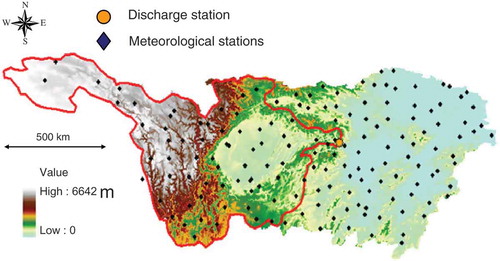
The test area is the Upper Yangtze River basin, China, gauged at Yichang, where the Three Gorges Dam is located. The basin is delimited by a continuous line in Fig. 1. The total area is about 1 005 500 km². The main river length is 2400 km, with an average discharge of 13 200 m³ s^-1 and a mean annual precipitation of about 800 mm, concentrated during the monsoon period when flood events are frequent. The basin drains a region of which 60% is mountainous and 40% agricultural plains (Jiang et al. 2007, Xu et al. 2008).

Fig. 1 DEM of the Upper Yangtze River basin with the meteorological and hydrological stations.

2.1 Meteorological ground stations

Daily meteorological data of rainfall, air temperature, relative air humidity and horizontal wind velocity are available from 1 January 2000 to September 2010 from the NDCD database (http://www.ncdc.noaa.gov/oa/ncdc.html). Daily incident short-wave solar radiation, which is needed for energy balance computation, is computed with the Allen (1997) equation using maximum and minimum daily air temperature and the extraterrestrial radiation.

The FEST-EWB hydrological model should be run at the hourly scale given the basic idea of the project to calibrate the soil and vegetation parameters using instantaneous satellite data of LST. The daily meteorological data are rescaled at the hourly scale. Specifically, for air temperature estimation, the method proposed by De Wit et al. (1978) is used, which is based on a sinusoidal algorithm considering sunrise and sunset hours. The Baig et al. (1991) model is used for incoming shortwave radiation computation based on a Gaussian curve. Rainfall, wind velocity and relative air humidity are assumed constant during the day.

Only 71 meteorological stations are available in this big basin, a very low spatial density compared to European or US river basins (Fig. 1).

Discharge measurements are available at Yichang station (30.66°N, 111.23°E) where the Three Gorges Dam is located, from 1 January 2000 to 31 December 2004 and for the year 2006, before construction of the dam.

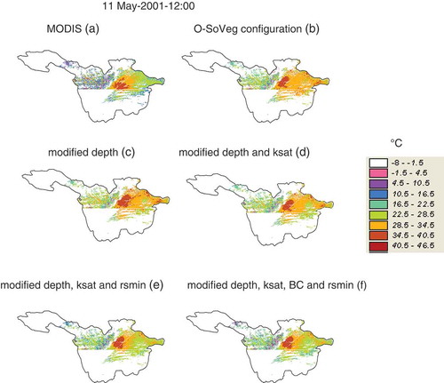
Fig. 2 MODIS LST (a) and RET images for the O-SoVeg configuration (b) and for some significant simulations (modified Depth (c), modified Depth and k_sat (d), modified Depth, k_sat and rs_min (e), modified Depth, k_sat, BC and rs_min (f)) for 11 May 2001 at 12:00.

2.2 Soil database and hydraulic properties

Available digital cartographic data include the digital elevation model (DEM) that has been developed at the US Geological Survey’s (USGS) EROS Data Center as a 30 arc-second DEM of the world (GTOPO30). Flow directions, slope and aspect were computed starting from the DEM resampled at a spatial resolution of 5000 m × 5000 m.

The pedological characteristics of the soils are available from the Harmonized World Soil Database (HWSD; FAO 2009). For the Yangtze River basin only three main classes can be identified: the soil texture is predominantly (for 94.5% of the region) in the sandy clay loam class, while only 2% has sand soils and 3.5% clay soils. From this available basic thematic layer, hydraulic soil parameters required for the application of the hydrological model were derived using the well-known database of Rawls and Brakensiek (1985), quantifying the saturated hydraulic conductivity, residual and saturated soil moisture, pore size distribution index, wilting point, field capacity and the Brooks-Corey index. In Table 1 the parameters subjected to calibration are reported.

Table 1 Saturated hydraulic conductivity (k_sat), active soil depth (Depth), minimum stomatal resistance (rs_min) and Brooks-Corey index (BC) for the three considered soil classes (mean values are reported together with the relative standard deviations in brackets). O-SoVeg: original soil–vegetation parameters.

Calibration procedure	ksat (m s^-1)	Depth (m)	BC	rsmin
O-SoVeg configuration	2.37 × 10^-6 (9.9 × 10^-6)	0.52 (0.16)	0.36 (0.11)	130.7 (49.6)
Modified parameters (calibration against LST)	1.92 × 10^-6 (4.3 × 10^-5)	0.75 (0.5)	0.24 (0.19)	85.9 (74.9)
10Ksat – 2Depth (calibration against Q)	2.37 × 10^-5 (9.9 × 10^-6)	1.04 (0.16)	0.36 (0.11)	130.7 (49.6)

2.3 Vegetation parameters

The land cover map for the Yangtze River basin was derived from the ESA Globcover Land Cover which was generated from the 300-m MERIS time series for the period between 2005 and June 2006 (Arino et al. 2007), with 22 land cover types defined according to the UN Land Cover Classification System. From this classification, vegetation height (h_v) and minimum stomatal resistance (rs_min) are defined for each type of vegetation. Twelve maps of h_v have been defined, one per month.

Leaf area index (LAI) maps were retrieved from the MODIS LAI products generated over an 8-day compositing period with a spatial resolution of 1 km aggregated at 5 km (http://ladsweb.nascom.nasa.gov/index.html). Images were taken every 16 days. Albedo (r) maps were retrieved from the MODIS white-sky product over an 8-day compositing period at 5 km (Liang 2001).

2.4 MODIS land surface temperature data

Land surface temperature was retrieved from MODIS LST daily L3 global 1km sin grid v004. Land surface temperature was retrieved from MODIS on board the satellites TERRA and AQUA with a spatial resolution of 1 km in the thermal infrared bands (Barnes et al. 1998). In total, 528 day-time and nocturnal images of MODIS11 LST products were selected for the whole simulation period from January 2000 to December 2010, and 170 images collected during the calibration period from 2000 to 2004. The images have been aggregated at the same spatial resolution as the FEST-EWB model simulations, i.e. 5 km, computing the mean value of the included pixels at 1 km.

3 MATERIAL AND METHODS

3.1 FEST-EWB hydrological model

The FEST-EWB model is a distributed hydrological energy water balance model (Corbari et al. 2010, 2011, 2013) and was developed starting from FEST-WB (Mancini 1990, Rabuffetti et al. 2008). The FEST-EWB model computes the main processes of the hydrological cycle: evapotranspiration, infiltration, surface runoff, flow routing, subsurface flow (Ravazzani et al. 2011) and snow dynamics (Corbari et al. 2009). The model is distributed so that the computation domain is discretized with a mesh of regular square cells in each of which every parameter is defined or calculated.

The input parameters of the model are: (a) meteorological variables, such as air temperature, incoming shortwave radiation, wind velocity, precipitation and air humidity; (b) the soil parameters in distributed maps, such as the saturated hydraulic conductivity (k_sat), the field capacity (fc), wilting point (wp), residual (θ_r) and saturated (θ_s) soil water content, Brooks-Corey index (BC), bubbling pressure (bp) and soil depth (Depth); (c) the vegetation parameters, such as LAI, vegetation height, minimum stomatal resistance (rs_min) and albedo; and (d) the digital elevation model (DEM) and land-use/land-cover map.

The core of the model is the system between the water and energy balance equations which are linked through evapotranspiration. In the energy balance between the soil surface, vegetation and near-surface atmosphere, all the terms are computed and the equation is solved looking for a representative equilibrium temperature that is the LST that closes the energy balance equation. This equilibrium surface temperature, which is an internal model variable, is comparable to LST as retrieved from operational remote sensing data at different spatial and temporal resolutions.

Soil moisture (SM) evolution for a generic cell at position i,j is described by the system between the energy and water balance equations:

(1)

where P is the precipitation rate (mm h^-1); R is the runoff flux (mm h^-1); PE is the drainage flux (mm h^-1); ET is the evapotranspiration rate (mm h^-1); z is the soil depth (m); Rn (W m^-2) is the net radiation; G (W m^-2) is the soil heat flux; H (W m^-2) and LE (W m^-2) are, respectively, the sensible heat and latent heat fluxes; and ΔW/Δt (W m^-2) encloses the energy storage terms which cannot be computed for this large basin. All these terms of the system are functions of the input soil and vegetation parameters.

Evaoptranspiration (ET) is linked to the latent heat flux (LE) through the latent heat of vaporization (λ) and the water density (ρ_w):

(2)

The latent heat flux (LE), as reported in Corbari et al. (2011), is then computed as:

(3)

where ρ_a is the air density; γ is the psychometric constant (Pa °C^-1); f_v is the vegetation fraction; c_p is the specific heat of humid air (MJ kg^-1 K^-1); the saturation vapour pressure, e* is computed as function of RET (Brutsaert 2005) and vapour pressure, e_a, as a function of air temperature; r_c is the canopy resistance, expressed following Jarvis (1976); r_s is the soil resistance according to Sun (1982); and the aerodynamic resistance (r_a for vegetation and r_abs for bare soil) is computed using the model from Thom (1975).

The sensible heat flux is computed as:

(4)

where T_a is the air temperature (°C).

The net radiation is computed as the algebraic sum of the incoming and outgoing shortwave and longwave radiation:

(5)

where R_s is the incoming shortwave radiation (W m^-2); r is albedo; ξ_c is the atmosphere emissivity; ξ_s is surface emissivity; and σ is the Stefan-Boltzmann constant (W m^-2 K^-4). Shortwave net radiation is calculated considering the effect of topography (Corbari et al. 2011).

The soil heat flux is the heat exchanged by conduction with the subsurface soil and is evaluated as:

(6)

where g_term is soil thermal conductivity (W m^-1 K^-1) and T_soil is soil temperature (°C) at 10 cm depth.

Thus, all the terms of the energy balance depend on RET and the energy balance equation can be solved looking for the thermodynamic equilibrium temperature that closes the equation with the Newton-Raphson method:

(7)

where RET_n is the actual value, RET_n-1 is the value at the previous iteration, f_t(RET_n-1) is the energy balance function and f_t′(RET_n-1) is its derivative. The solution is acceptable when:

with tolerance equal to 0.001.

The runoff routing throughout the hillslope and the river network is performed via a diffusion wave scheme based on the Muskingum-Cunge method in its nonlinear form with time variable celerity; details are given by Montaldo et al. (2007). Runoff is computed according to a modified SCS-CN method extended for continuous simulation (Ravazzani et al. 2007), where the potential maximum retention is updated cell by cell at the beginning of rainfall as a linear function of the degree of saturation.

The subsurface flow routing is computed with a linear reservoir routing scheme governed by the constant value k_prof which is a function of the ratio between cell dimension and inclination multiplied by the hydraulic conductivity for deep soil. The subsurface flow is computed only in sloping cells where the influence of the inclination of the mountainside is relevant, while in the plain this subsurface flow is not computed.

The FEST-EWB model was proved to make accurate predictions of actual evapotranspiration by comparisons against energy and mass exchange measurements acquired by an eddy covariance station (Corbari et al. 2011), and also at the agricultural district scale by comparisons with ground and remote sensing information (Corbari et al. 2010).

3.2 Calibration and validation methodology

3.2.1 Calibration strategies

At the basin scale, satellite images of LST provide the opportunity to calibrate distributed hydrological models in each pixel of the domain as a complementary method to traditional calibration with discharge measurements at the few available control cross-sections.

So the innovative contribution of this article is the possibility to calibrate model internal state variables (e.g. land surface temperature) in addition to the traditional external fluxes (e.g. discharge) to obtain better understanding of hydrological processes and model analysis at the pixel scale (Dooge 1986, Refsgaard 1997). The traditional calibration based only on river discharge data in a few rivers sections lumps all the hydrological processes together, so that the correct spatial determination of mass and energy fluxes becomes more difficult. When a pixel-by-pixel calibration is performed, a better spatial distribution should be achieved. The proposed methodology is based on a pixel-by-pixel scale modification of soil and/or vegetation parameters through comparison of the model internal state variable RET and the remotely observed LST. This procedure for the calibration of soil hydraulic parameters, and so of LST and soil water content, is based on a trial-and-error approach. Different percentages of change for the different ranges of differences between LST and RET are tested in different simulations based on random choice.

The procedure can be divided into four steps:

1. the FEST-EWB model is run in the configuration with the original soil–vegetation parameters (O-SoVeg);

2. RET is compared with LST from MODIS in each pixel of the domain, and statistical parameters, histograms and spatial autocorrelation functions are computed;

3. soil and/or vegetation parameters are modified differently in each pixel of the domain in order to minimize errors between observed and modelled LST; and

4. FEST-EWB is run with the new configuration.

The procedure is then repeated from (b).

The parameters subjected to calibration are: soil hydraulic conductivity, Brooks-Corey index, soil depth and minimum stomatal resistance, which were selected from the sensitivity analysis (see Section 3.3). These are modified ensuring that their values remain within the physical ranges (Rawls and Brakensiek 1985).

The traditional calibration procedure based on comparison against ground observed flow data is also performed. In this calibration against discharge, each soil parameter is multiplied or divided by a factor which is constant for the entire basin, whereas in the LST calibration procedure, every single pixel is multiplied by a different factor according to the relative difference in terms of temperature.

Moreover, LST is a driving factor of the surface processes, especially during dry conditions, while discharges are a function of both the surface and subsurface processes that the LST cannot control alone. Given this context, to compare the two calibration strategies, a comparison of only surface flows is performed. The measured flow is divided into surface and basal flow using the methodology described in Lim et al. (2005). Only cumulated volumes of surface flow are considered, because in this analysis only water quantity is needed and not the timing of the flow hydrograph.

For the Upper Yangtze River basin, FEST-EWB was run at the hourly time step and with a spatial resolution of 5 km. Within the calibration period from 2000 to 2004, the period from 1 January to 31 July 2000 is considered as a warm-up period, due to the fact that the initial snow cover condition in the mountains is equal to zero. So the comparison between observed and simulated LST images and cumulated volumes starts from August 2000. The validation period is defined from January 2005 to September 2010.

3.2.2 Evaluation criteria

The goodness of the model estimates is evaluated through different statistical indexes which are computed for RET images as well as for cumulated volume of discharge. For the evaluation of simulated estimates, the mean bias error (MBE), the absolute mean bias error (AMBE), the root mean square error (RMSE) and the relative error (RE) are computed as follows:

(8)

(9)

(10)

(11)

where X_simⁱ is the ith simulated variable by FEST-EWB, X_obsⁱ is the ith measured variable, n the sample size, and the average observed variable.

Moreover the Nash-Sutcliffe index, η, is also computed according to (Nash and Sutcliffe 1970):

(12)

The Nash-Sutcliffe efficiency is commonly used to assess the predictive power of hydrological models. It can range from −∞ to 1. Essentially, the closer the model efficiency is to 1, the more accurate the model is.

3.3 Sensitivity analysis of RET and energy fluxes at local scale

A field-scale analysis was at first performed to understand the effects of the changes of soil and vegetation parameters on mass and energy fluxes (e.g. soil moisture and evapotranspiration). Data for the year 2006 from a micrometeorological station located in a corn field in northern Italy were used to calibrate the FEST-EWB model parameters. The station is equipped with sensors to measure air temperature and the three components of wind speed, net radiation, latent heat flux, sensible heat flux, ground heat flux, air humidity and soil water content every 30 min (Masseroni et al. 2012). Albedo is computed from the observed outgoing shortwave radiation. Soil texture was also analysed through ground measurement in the field and was categorized as sandy clay loam class. Using the database of Rawls and Brakensiek (1985), the following values were assigned to each soil hydraulic parameter: 0.972 × 10^-6 m s^-1 for saturated hydraulic conductivity; 0.2808 mm for bubbling pressure; 0.398 and 0.068 for saturated and residual soil water content, respectively; 0.319 for the Brooks-Corey index; and 0.148 and 0.255 for wilting point and field capacity, respectively. The minimum stomatal resistance for maize was fixed at a constant value of 100 s m^-1. Soil depth was set at 70 cm, which corresponds to the maximum length reached by maize roots. This configuration is referred to herein as the original soil–vegetation parameters for local simulation (O-SoVeg-local).

The other input vegetation parameters required for the FEST-EWB model are the vegetation height, LAI and vegetation fraction, which were measured in the field throughout the season.

A set of simulations was created by varying single soil or vegetation parameters and also combinations of these parameters. Table 2 lists 13 of the more significant simulations, and the absolute and relative errors for net radiation, latent and sensible heat fluxes, ground heat flux, soil moisture and LST are computed for each simulation with respect to the simulation performed with the O-SoVeg-local configuration. From these analyses, it seems that the net radiation is the variable least affected by changes in soil and vegetation parameters, with variations ranging between 1% and 4.7%. In contrast, the ground and the sensible heat fluxes undergo large changes of between 15% and 141.3%. Latent heat flux, LST and soil moisture show a similar degree of variability of 10% to 20%. A decrease of saturated hydraulic conductivity (simulations 1 and 2) leads to an increase in latent heat flux and, of course, a decrease in sensible heat flux, which causes a negative change of LST. The opposite variations in the same variables are found when k_sat is multiplied by a factor of 10. The Brooks-Corey index (Simulation 4), which affects percolation, produces a change in latent heat flux similar to Simulation 1, with a change in k_sat, but the soil moisture has a slightly smaller increase. This is also true if the minimum stomatal resistance is considered. The parameters that affect the representative equilibrium temperature more are the saturated hydraulic conductivity and the soil depth. If more parameters are modified simultaneously, the variations of energy and mass flux estimates increase. For example, in Simulation 13, which takes into account all the changed parameters, greater changes in LST and latent heat flux are reported.

Table 2 Absolute and relative errors with respect to the O-SoVeg configuration of simulations at the local scale and changes in the soil and vegetation parameters.

Modified parameters	Absolute error % (relative error %)
	Rnet	LE	H	G	SM	RET
ksat/10	2.4	14.6	77.2	64.0	19.4	6.3
	(0.01)	(10.2)	(–89.3)	(–8.6)	(14.5)	(–0.7)
ksat/100	3.2	16.8	101.8	89.2	39.4	7.4
	(–0.1)	(16.2)	(–4.3)	(–10.7)	(30.04)	(–1.3)
ksat × 10	2.2	13.9	63.0	53.0	17.4	6.8
	(–0.01)	(–10.2)	(75.2)	(9.2)	(–10.1)	(0.9)
BC × 0.637	2.2	14.6	65.1	55.8	9.4	6.5
	(–16.0)	(2.1)	(–5.1)	(7.9)	(6.9)	(–0.5)
Depth × 2	3.3	17.6	102.8	87.1	21.1	7.6
	(–1.1)	(–28.4)	(2.3)	(–640.8)	(11.6)	(1.2)
rsmin = 50	1.9	13.3	63.1	15.7	0.6	5.0
	(–0.3)	(0.2)	(–96.6)	(3.7)	(–1.3)	(–0.2)
rsmin = 200	3.0	20.7	90.3	30.5	1.8	6.6
	(1.6)	(1.7)	(–6.2)	(6.9)	(2.1)	(–0.4)
(ksat/10) – (BC × 0.637)	2.7	15.2	85.0	83.5	25.7	7.0
	(–0.9)	(20.4)	(–5.3)	(–72.4)	(18.8)	(–1.0)
(ksat/10) – (Depth × 2)	4.4	24.7	141.3	89.3	42.2	8.4
	(–0.4)	(–10.3)	(–613.1)	(–7.5)	(33.3)	(–1.6)
(ksat/10) – (BC × 0.637) – rsmin = 50	3.0	19.3	103.2	86.0	21.6	7.1
	(–0.9)	(15.8)	(11.1)	(–64.0)	(16.4)	(–1.4)
(ksat/10) – (BC × 0. 637) – rsmin = 50 – depth × 2	5.0	20.1	80.1	84.0	39.4	8.8
	(–0.5)	(18.8)	(–90.3)	(–9.6)	(18.5)	(–1.7)

4 RESULTS

4.1 Calibration through comparison between RET and LST from MODIS

The calibration of soil hydraulic and vegetation parameters for the Yangtze River basin is reported here, showing the comparison between RET estimates from the FEST-EWB model and MODIS satellite data of LST that were chosen as the benchmark in this study.

In Fig. 2, as an example, the RET image for 11 May 2001 at 12:00 is reported for the O-SoVeg configuration, as well as the LST image from MODIS. The hydrological model seems to be able to reproduce the different thermodynamic behaviours differentiating between mountains with lower temperature, and plains with higher temperature, and it is clear from the legend that the values are different. If histograms are computed (Fig. 3), a discordant distribution of pixel numbers is found between RET and MODIS LST in each temperature class. The classes are composed of temperature ranges of 2°C. Table 3 reports the evaluation parameters computed for the Upper Yangtze River basin for RET from the FEST-EWB model in the original O-SoVeg configuration. Values of MBE and AMBE indicate a mean overestimation, respectively, of 0.4 and 4.5°C for the entire dataset of 170 images; RMSE = 5.3°C; the relative error is 18.4%; and the Nash-Sutcliffe index is equal to 0.15.

Fig. 3 Histograms for MODIS LST (a) and RET images for the O-SoVeg configuration (b) and for some significant simulations (modified Depth (c), modified Depth and k_sat (d), modified Depth, k_sat and rs_min (e), modified Depth, k_sat, BC and rs_min (f)) for 11 May 2001 at 12:00.

Table 3 Mean bias error (MBE), absolute mean bias error (AMBE), root mean square error (RMSE), relative error (RE) and Nash-Sutcliffe index (η) computed for 170 images of the Yangtze River basin for the calibration period—O-SoVeg configuration.

O-SoVeg configuration	MBE (°C)	AMBE (°C)	RMSE (°C)	RE (%)	η
Complete database	0.4	4.4	5.9	18.4	0.15
Day-time images	0.1	5.2	6.8	18.9	0.11
Night-time images	0.7	3.6	4.9	18.1	0.18
Summer images	−0.5	4.0	5.5	17.2	0.14
Winter images	1.1	4.8	6.3	18.9	0.17

An initial deeper analysis can be performed considering errors computed only for night-time images and for day-time maps. In fact, the thermodynamic variability that is clearly evident during the day is softened at night. So higher errors are present during the day, with AMBE of 5.2°C and RMSE of 6.8°C, while an AMBE of 3.6°C is reached at night with RMSE of 4.9°C (Table 3). A substantial difference in terms of temperature is, of course, also present between summer and winter. This variability is accentuated by the large variations in altitude in the Upper Yangtze River basin, from about 6200 m a.s.l. to 500 m a.s.l. The images database was divided into two homogeneous groups, according to the mean LST of the basin between May and September and between October and March, for the four years of analysis. From the comparison between RET and MODIS LST, an AMBE of 4°C is found for summer periods and an overestimation of 4.8°C for winter images (Table 3).

Summarizing all the analyses performed, FEST-EWB in the O-SoVeg configuration generally overestimates LST from MODIS. So according to the methodology described in Section 3.2, the soil hydraulic and vegetation parameters are now modified differently in each pixel of the domain to minimize RMSE, MBE and AMBE and maximize the Nash-Sutcliffe index. The parameters subjected to calibration are: soil hydraulic conductivity, Brooks-Corey index, soil depth and minimum stomatal resistance. Each parameter is modified differently in each pixel, increasing or decreasing it by a different percentage based on the difference between the simulated and observed LST. More than 60 combinations of parameters and percentage of change have been tested. Table 4 lists some of the most interesting simulations, reporting which parameters are modified.

Table 4 Mean bias error (MBE), absolute mean bias error (AMBE), root mean square error (RMSE), relative error (RE) and Nash-Sutcliffe index (η) computed for 170 images of the Yangtze River basin for the calibration period—other simulations performed. (O-SoVeg included for comparison.)

Modified parameters	MBE (°C)	AMBE (°C)	RMSE (°C)	RE (%)	η
O-SoVeg	0.4	4.4	5.9	18.4	0.15
Modified ksat	0.63	4.2	5.1	17.9	0.19
Modified Depth	0.5	4.0	5.2	16.5	0.24
Modified Depth and ksat	0.48	3.3	4.8	10.4	0.31
Modified ksat and BC	0.6	4.0	5.1	16.2	0.22
Modified ksat, Depth and BC	0.43	3.1	4.3	10.6	0.34
Modified ksat, Depth and rsmin	0.3	2.9	3.7	9.1	0.49
Modified ksat, Depth, BC and rsmin	0.15	1.9	2.9	6.2	0.65

In Fig. 2, RET images for 11 May 2001 at 12:00 are also reported for some significant simulations showing how LST is affected by the changes in soil hydraulic and/or vegetation parameters. The differences between simulations are apparent in Fig. 3, in which histograms are shown for the same significant simulations as selected in Fig. 2. In fact the number of pixels in the different classes changes between the different simulations. The RET frequency distribution that denotes a more similar shape to that of LST from MODIS is related to simulation with the modified parameters of k_sat, Depth, BC and rs_min, where there is almost the same number of pixels in the different classes. The errors that confirm this finding are given in Table 5 for the different FEST-EWB model configurations and for MODIS. A strong decrease in AMBE is shown from the simulation in the O-SoVeg configuration, with AMBE = 5.4°C, to the simulation with the modified parameters of k_sat, Depth, BC and rs_min, with AMBE = 1.8°C, as well as for the other statistical parameters. The parameter values for the entire basin reported in Table 1 show an increase in the spread of the parameters with respect to the original values. In fact higher standard deviations of the parameters are linked to the methodology of calibration based on the LST difference in each pixel.

Table 5 Mean bias error (MBE), absolute mean bias error (AMBE), root mean square error (RMSE), relative error (RE) and Nash-Sutcliffe index (η) computed for 11 May 2001 at 12:00 h.

Modified parameters	MBE (°C)	AMBE (°C)	RMSE (°C)	RE (%)	η
O-SoVeg	−2.81	5.4	6.9	−19.1	−0.02
Modified Depth	−2.0	4.1	6.1	−16.3	0.10
Modified Depth and ksat	−1.94	3.9	5.2	−14.6	0.22
Modified ksat, Depth and BC	−0.8	2.8	3.1	−12.1	0.49
Modified ksat, Depth, BC and rsmin	0.6	1.8	2.4	−4.3	0.71

In Fig. 4the mean absolute differences between RET from FEST-EWB and LST from MODIS are reported for the 4-year calibration period. From these analyses performed on histograms and statistical indices, the parameters that minimize AMBE (1.9°C), MBE (0.15°C), RMSE (2.9°C), RE (6.2%) and that maximize the Nash-Sutcliffe index (0.65) are linked to the modification of k_sat, Depth, BC and rs_min. The statistical results for some simulations are reported for the 170 dates in Table 4.

Fig. 4 Absolute mean differences between LST from the FEST-EWB model and LST from MODIS satellite data for the 4-year of simulation period.

The statistical parameters are also computed separating between day-time and night-time images, and between summer and winter periods, and a good ability of the model in reproducing satellite data is observed for each situation (Table 6).

Table 6 Mean bias error (MBE), absolute mean bias error (AMBE), root mean square error (RMSE), relative error (RE) and Nash-Sutcliffe index (η) computed for 170 images for the calibration phase for the selected simulation with the modification of k_sat, Depth, BC and rs_min.

Modified ksat, depth, BC and rsmin	MBE (°C)	AMBE (°C)	RMSE (°C)	RE (%)	η
Complete database	0.15	1.9	2.9	6.2	0.65
Day-time images	0.31	2.4	3.1	7.1	0.6
Night-time images	0.1	1.6	2.6	6.1	0.68
Summer images	0.28	2.3	3.1	7.0	0.62
Winter images	0.21	2.0	3.2	7.1	0.66

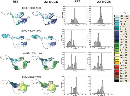
The evaluation parameters are confirmed by frequency distributions graphs. Exampes of RET maps from the selected simulation are shown in Fig. 5, accompanied by the corresponding histogram for some dates showing a good similarity between simulated and observed LST for night-time as well as day-time images. A good performance is also reported for summer time, when greater thermodynamic variability is present.

Fig. 5 Examples of RET and LST MODIS maps from the selected simulation, with the corresponding histograms.

4.2 Calibration through the comparison between observed and simulated discharge volume

The FEST-EWB model was also calibrated following the traditional methodology, based on comparison between observed and simulated discharge cumulated volume in river cross-sections, which has been well assessed by the scientific community (Beven and Binley 1992, Brath et al. 2004, Rabuffetti et al. 2008). For the Yangtze River basin the Yichang station was selected due to availability of observed data in only that cross-section.

In this calibration against discharge procedure, each soil parameter is multiplied or divided by a factor which is constant for the entire basin. This procedure differs from the proposed methodology based on LST, in which each pixel is multiplied by a different factor according to the relative difference in terms of temperature.

The calibration on discharge is based on a trial-and-error approach. The comparison is primarily focused on flood volumes, which are strongly dependent on the infiltration process, and not linked with the timing of propagation. The parameters subjected to calibration are the soil hydraulic conductivity, Depth, rs_min and BC. These parameters have been modified taking into account that an increase in deep soil conductivity implies an increase in subsurface flow, and a decrease in k_sat leads to an increase in the drainage process. The CN map and parameters required for surface flow routing (roughness coefficient and section width) were not modified in the calibration process.

Each simulation was then compared with the observed cumulated volume, and the quality indices calculated to classify the model reliability. In this framework, negative relative errors for discharge volumes show that the model tends to underestimate observed data. In Table 7, relative errors between observed volume and simulated volumes from FEST-EWB runs in the O-SoVeg configuration, and after the calibration process against discharge, are reported. Before calibration, it seems that the FEST-EWB model tends to underestimate cumulated volume over 4 years, while model improvement can be seen with the calibration process. In fact, the calibration activity produced a general improvement in the model performance in terms of flood volume errors ranging from –77.9% to –8.7%. The simulation which minimizes the error on cumulated volume is characterized by the modified soil parameters: k_sat multiplied by 10 and Depth by 2. The parameter values for the entire basin along with their standard deviations after calibration against Q are also reported in Table 1. The spatial variation of the parameters does not change; in fact the standard deviation remains the same as for the original values.

Table 7 Relative errors in surface volume between observed and simulated using FEST-EWB for the simulations with the original parameters, and calibrated against LST and Q.

	Calibration (September 2000–2004)		Validation (2006)
	RE (%) on discharge volumes	η	RE (%) on discharge volumes	η
O-SoVeg configuration	−27.9	0.54	−25.5	0.58
modified ksat, Depth, BC and rsmin (calibration against LST)	3.0	0.81	2.9	0.79
Ksat × 10 – Depth × 2 (calibration against Q)	−6.3	0.62	−7.6	0.63

In Table 7, errors in cumulated volume are also reported for the selected simulation after the pixel-to-pixel calibration process against LST from MODIS where k_sat, BC, rs_min and Depth have been modified.

In Fig. 6 the observed cumulated volume is shown together with the selected FEST-EWB simulations after the calibrations performed against river discharge and against satellite LST images. The simulation period from 1 January to 31 July 2000 is considered to be a start-up period, due to the fact that the initial snow cover condition is zero; thus the statistical parameters are computed starting from 1 August 2000.

Fig. 6 Observed cumulated surface volume, together with selected FEST-EWB simulations from both the internal and external validation processes.

4.3 Validation

For the validation period (January 2005–September 2010), 358 MODIS LST images were selected. The RET from the FEST-EWB model with the calibrated parameters (modified k_sat, BC, rs_min and Depth) were then compared with MODIS data and the statistical indices computed, as follows: AMBE = 2.3°C, MBE = 0.32°C, RMSE = 3.6°C and RE = 9.2%. These results confirm the goodness of the performed calibration. The results are also analysed in terms of surface cumulated volume for the year 2006, for which observed data are available. In Table 7, the relative errors (RE) show that the simulation calibrated against LST slightly outperforms the observed cumulated volume (2.9%), while the simulation calibrated against Q underestimates it (–7.6%). It is also interesting to note the difference in η index, which indicates that the surface volume obtained from the FEST-EWB model calibrated against LST has a shape more similar to the observed one than the volume computed from FEST-EWB calibrated against Q.

5 DISCUSSION

The advantage of performing an internal validation of the FEST-EWB model using satellite LST has been shown. Following the direction highlighted by Dooge (1986), we have tried to analyse the behaviour of the model internal state variable (e.g. soil moisture and its proxy) in addition to the traditional external fluxes (e.g. discharge) to better understand the hydrological processes in each pixel of the domain.

The FEST-EWB model calibrated using LST retrieved from MODIS satellite sensor data performed quite well. These results should be seen in the context of hydrological simulations, where the ultimate goal is estimates of distributed evapotranspiration, water content and local discharge. As reported in Section 3.3, if the uncertainty in the RET estimate is analysed in terms of relative errors, a variation of about 1% in RET can lead to a difference in the LE estimate of between 10% and 20%. In terms of values, Corbari et al. (2011) showed that a bias of 2.5°C in LST estimates leads to an error of only about 20 W m^-2 in LE computation in FEST-EWB. Similar results are reported in the literature where, for example, Brutsaert et al. (1993) report that a variation of 0.5 K in LST can lead to an error of 10% in sensible heat flux estimation.

Furthermore, the MODIS images uncertainty linked to the retrieval algorithm should also be taken into account. The definition of satellite LST over a heterogeneous area should be analysed considering the spatial resolution, angle of view of the sensor and emissivity (Sobrino et al. 1994, Jacob et al. 2004, Kustas et al. 2004, Sòria and Sobrino 2007). Sobrino et al. (2007) analysed the accuracy of MODIS LST products, showing that the mean bias with ground data is equal to 2 K. Wang et al. (2008) report an extensive validation of different MODIS LST products with biases between 0.8 and 3°C, and RMSE around 2°C.

In the present research, thermal infrared data were selected instead of a direct estimate of surface soil moisture inferred from microwave data, because, despite its potential (mainly overcoming cloud cover problems contaminating thermal infrared images), many limitations are present due to the complex geometry of the readings, low sensitivity to soil water content above a threshold significant for flood generation (Mancini et al. 1999), and low spatial resolution (Wagner and Scipal 2000). Moreover other limitations are linked to the signal penetration into the soil, so that SM values from microwave information are related to the upper centimetres only (Wagner et al. 1999) and also to the noise signal due to vegetation (Jackson et al. 1982).

Another problem linked to the application to the Yangtze River basin is related to the selected spatial resolution of 5 km. This means that a problem of spatial representativeness appears due to the process of aggregation from the nominal resolution of LST MODIS images of 1 km to 5 km. The aggregation was performed using the mean value of the 1 km × 1 km pixels enclosed in the 5 km × 5 km pixel.

A big part of the uncertainty is also due to the available ground meteorological data. Two problems can be highlighted: (a) the small number of stations which do not cover the entire basin, and (b) the downscaling procedure applied to daily data to compute hourly data. A source of error can also be found in the definition of the pedological characteristics of the basin soils from the Harmonized World Soil Database, due to the fact that only three types of soil are identified and more 94.5% of the basin is included in only one class.

Problems also arise from the calibration performed using discharge measurements. It is well known from the literature that ground data of river flow are affected by high uncertainty (Beven 2006, Di Baldassarre and Montanari 2009). Pelletier (1988), after reviewing 140 publications on river discharge errors, found that the uncertainty ranges between 8% and 20%. Baldassarre and Montanari (2009) highlighted that errors along the Po River are between 6.2% and 42.8%. We did not find errors for Yangtze River discharge reported in the literature, but some error should be taken into account.

6 CONCLUSIONS

In this study, the FEST-EWB model was calibrated for the Upper Yangtze River basin using satellite imagery of land surface temperature (LST), as well as river discharge measurements.

A procedure for the internal calibration of the hydrological processes is presented so that soil hydraulic parameters and vegetation variables are calibrated differently in each pixel according to the comparison between observed LST and simulated RET, minimizing the errors. The calibration procedure based on LST seems to outperform the calibration based on discharge, with lower relative error and a higher Nash-Sutcliffe index on cumulated volume. Using this methodology, a different spatial distribution of soil and vegetation parameters can be obtained.

This methodology will be of particular interest in ungauged basins where satellite LST can now be used to calibrate the evaporative processes in each pixel of the domain without river discharge being known. It also raises the possibility of using LST from remote sensing for driving irrigation management differentiating between the different plots.

Additional information

Funding

This work was supported in the framework of the Dragon 2 Programme between the European Space Agency (ESA) and the National Remote Sensing Centre of China (NRSCC).

REFERENCES

- Allen, R.G., 1997. Self calibrating method for estimating solar radiation from air temperature. Journal of Hydrologic Engineering, 2 (2), 56–67. doi:10.1061/(ASCE)1084-0699(1997)2:2(56).
- Arino, O., et al., 2007. GlobCover: ESA service for global land cover from MERIS. In: Geoscience and Remote Sensing Symposium, 11–16 July, Boston, MA. 2412–2415.
- Baig, A., Akhter, P., and Mufti, A., 1991. A novel approach to estimate the clear day global radiation. Renewable Energy, 1, 119–123. doi:10.1016/0960-1481(91)90112-3.
- Barnes, W.L., Pagano, T.S., and Salomonson, V.V., 1998. Prelaunch characteristics of the moderate resolution imaging spectroradiometer (MODIS) on EOS-AM1. IEEE Transactions on Geoscience and Remote Sensing, 36 (4), 1088–1100. doi:10.1109/36.700993.
- Bastiaanssen, W.G.M., 1998. A remote sensing surface energy balance algorithm for land (SEBAL), 1. Formulation. Journal of Hydrology, 212–213, 198–212. doi:10.1016/S0022-1694(98)00253-4.
- Beven, K.J., 2006. A manifesto for the equifinality thesis. Journal of Hydrology, 320, 18–36. doi:10.1016/j.jhydrol.2005.07.007.
- Beven, K. and Binley, A., 1992. The future of distributed models: model calibration and uncertainty prediction. Hydrological Processes, 6, 279–298. doi:10.1002/hyp.3360060305.
- Brath, A., Burlando, P., and Rosso, R., 1998. Sensitivity analysis of real time flood forecasting to on-line rainfall predictions. In: F. Siccardi and R.L. Bras, eds. Selected papers from the workshop on Natural disasters in European Mediterranean countries, 27 June–1 July 1988, Perugia. 469–488.
- Brath, A., Montanari, A., and Toth, E., 2004. Analysis of the effects of different scenarios of historical data availability on the calibration of a spatially-distributed hydrological model. Journal of Hydrology, 291, 232–253. doi:10.1016/j.jhydrol.2003.12.044.
- Brutsaert, W., 2005. Hydrology: an introduction. Cambridge: Cambridge University Press.
- Brutsaert, W., Hsu, A., and Schmugge, T.J., 1993. Parameterization of surface heat fluxes above forest with satellite thermal sensing and boundary-layer soundings. Journal of Applied Meteorology and Climatology, 32 (5), 909–917. doi:10.1175/1520-0450(1993)032<0909:POSHFA>2.0.CO;2.
- Caparrini, F., Castelli, F., and Entekhabi, D., 2004. Estimation of surface turbulent fluxes through assimilation of radiometric surface temperature sequences. Journal of Hydrometeorology, 5, 145–159. doi:10.1175/1525-7541(2004)005<0145:EOSTFT>2.0.CO;2.
- Castillo, V.M., Gomez-Plaza, A., and Martinez-Mena, M., 2003. The role of antecedent soil water content in the runoff response of semiarid catchments: a simulation approach. Journal of Hydrology, 284 (1–4), 114–130. doi:10.1016/S0022-1694(03)00264-6.
- Ciarapica, L. and Todini, E., 2002. TOPKAPI: a model for the representation of the rainfall-runoff process at different scales. Hydrological Processes, 16, 207–229. doi:10.1002/hyp.342.
- Corbari, C., et al., 2009. Elevation based correction of snow coverage retrieved from satellite images to improve model calibration. Hydrology and Earth System Sciences, 13, 639–649. doi:10.5194/hess-13-639-2009.
- Corbari, C., et al., 2010. Land surface temperature representativeness in a heterogeneous area through a distributed energy-water balance model and remote sensing data. Hydrology and Earth System Sciences, 14, 2141–2151. doi:10.5194/hess-14-2141-2010.
- Corbari, C., et al., 2013. Mass and energy flux estimates at different spatial resolutions in a heterogeneous area through a distributed energy–water balance model and remote-sensing data. International Journal of Remote Sensing, 34 (9–10), 3208–3230. doi:10.1080/01431161.2012.716924.
- Corbari, C., Ravazzani, G., and Mancini, M., 2011. A distributed thermodynamic model for energy and mass balance computation: FEST-EWB. Hydrological Processes, 25, 1443–1452. doi:10.1002/hyp.7910.
- Crow, W.T., Kustas, W.P., and Prueger, J.H., 2008. Monitoring root-zone soil moisture through the assimilation of a thermal remote sensing-based soil moisture proxy into a water balance model. Remote Sensing of Environment, 112 (4), 1268–1281. doi:10.1016/j.rse.2006.11.033.
- Crow, W.T., Wood, E.F., and Pan, M., 2003. Multiobjective calibration of land surface model evapotranspiration predictions using streamflow observations and spaceborne surface radiometric temperature retrievals. Journal of Geophysical Research-Atmosphere, 108, D23. doi:10.1029/2002JD003292.
- De Wit, C.T., Goudrian, J., and Van Laar, H.H., 1978. Simulation of respiration and transpiration of crops. Wangeningen: Pudoc, 148 pp.
- Di Baldassarre, G. and Montanari, A., 2009. Uncertainty in river discharge observations: a quantitative analysis. Hydrology and Earth System Sciences, 13, 913–921. doi:10.5194/hess-13-913-2009.
- Dooge, J.C.I., 1986. Looking for hydrologic laws. Water Resources Research, 22 (9S), 46S–58. doi:10.1029/WR022i09Sp0046S.
- Famiglietti, J.S. and Wood, E.F., 1994. Multiscale modeling of spatially variable water and energy balance processes. Water Resources Research, 30, 3061–3078. doi:10.1029/94WR01498.
- FAO/IIASA/ISRIC/ISSCAS/JRC, 2009. Harmonized World Soil Database (version 1.1). FAO, Rome and IIASA, Laxenburg. Available from: http://www.iiasa.ac.at/Research/LUC/External-World-soil-database/HTML
- Franks, S.W. and Beven, K.J., 1999. Conditioning a multiple-patch SVAT Model using uncertain time-space estimates of latent heat fluxes as inferred from remotely sensed data. Water Resources Research, 35 (9), 2751–2761. doi:10.1029/1999WR900108.
- Giacomelli, A., et al., 1995. Evaluation of surface soil moisture by means of SAR remote sensing techniques and conceptual modelling. Journal of Hydrology, 166, 445–459.
- Gutmann, E.D. and Small, E.E., 2010. A method for the determination of the hydraulic properties of soil from MODIS surface temperature for use in land surface models. Water Resources Research, 46, W06520. doi:10.1029/2009WR008203.
- Jackson, T.J., Schmugge, T.J., and Wang, J.R., 1982. Passive microwave sensing of soil moisture under vegetation canopies. Water Resources Research, 18 (4), 1137–1142. doi:10.1029/WR018i004p01137.
- Jacob, F., 2004. Comparison of land surface emissivity and radiometric temperature derived from MODIS and ASTER sensors. Remote Sensing of Environment, 90, 137–152. doi:10.1016/j.rse.2003.11.015.
- Jarvis, P.G., 1976. The interpretation of the variations in leaf water potential and stomatal conductance found in canopies in the field. Philosophical Transactions of the Royal Society B: Biological Sciences, 273, 593–610. doi:10.1098/rstb.1976.0035.
- Jiang, T., Su, B., and Hartmann, H., 2007. Temporal and spatial trends of precipitation and river flow in the Yangtze River Basin, 1961–2000. Geomorphology, 85 (3–4), 143–154. doi:10.1016/j.geomorph.2006.03.015.
- Kalma, J.D., McVicar, T.R., and McCabe, M.F., 2008. Estimating land surface evaporation: a review of methods using remotely sensed surface temperature data. Surveys in Geophysics, 29, 421–469. doi:10.1007/s10712-008-9037-z.
- Kerr, Y.H., et al., 2001. Soil moisture retrieval from space: the soil moisture and ocean salinity (SMOS) mission. IEEE Transactions on Geoscience and Remote Sensing, 39 (8), 1729–1735. doi:10.1109/36.942551.
- Kumar, P. and Kaleita, A.L., 2001. Assimilation of surface temperature in a land-surface model. In: M. Owe et al., eds. Remote sensing and hydrology 2000 (Proceedings of a symposium held at Santa Fe, New Mexico, USA, April 2000). Wallingford, UK: International Association of Hydrological Sciences, IAHS Publ. 267, 197–201 [Available at: http://iahs.info/uploads/dms/iahs_267_0197.pdf]
- Kustas, W.P., et al., 2004. Effects of remote sensing pixel resolution on modeled energy flux variability of croplands in Iowa. Remote Sensing of Environment, 92 (4), 535–547. doi:10.1016/j.rse.2004.02.020.
- Lakshmi, V., 2000. A simple surface temperature assimilation scheme for use in land surface models. Water Resources Research, 36 (12), 3687–3700. doi:10.1029/2000WR900204.
- Liang, S., 2001. Narrowband to broadband conversions of land surface albedo I. Remote Sensing of Environment, 76, 213–238. doi:10.1016/S0034-4257(00)00205-4.
- Liang, X., 1994. A simple hydrologically based model of land surface water and energy fluxes for general circulation models. Journal of Geophysical Research, 99, 14415–428. doi:10.1029/94JD00483.
- Lim, K.J., 2005. Automated web gis based hydrograph analysis tool, what. Journal of the American Water Resources Association, 41 (6), 1407–1416. doi:10.1111/j.1752-1688.2005.tb03808.x.
- Mancini, M., 1990. La modellazione distribuita della risposta idrologica: effetti della variabilità spaziale e della scala di rappresentazione del fenomeno dell’assorbimento. Thesis (PhD), Politecnico di Milano, Milan, (in Italian).
- Mancini, M., Hoeben, R., and Troch, P., 1999. Multifrequency radar observations of bare surface soil moisture content: a laboratory experiment. Water Resources Research, 35, 1827–1838. doi:10.1029/1999WR900033.
- Masseroni, D., et al., 2012. Turbulence integral length and footprint dimension with reference to experimental data measured over maize cultivation in Po Valley, Italy. Atmosfera, 25 (2), 183–198.
- Merlin, O., et al., 2005. A combined modeling and multispectral/multiresolution remote sensing approach for disaggregation of surface soil moisture: application to SMOS configuration. IEEE Transactions on Geoscience and Remote Sensing, 43 (9), 2036–2050. doi:10.1109/TGRS.2005.853192.
- Merlin, O., Walker, J, Chehbouni, A, Kerr, Y, 2008. Towards deterministic downscaling of SMOS soil moisture using MODIS derived soil evaporative efficiency. Remote Sensing of Environment, 112 (10), 3935–3946. doi:10.1016/j.rse.2008.06.012.
- Montaldo, N., Ravazzani, G., and Mancini, M., 2007. On the prediction of the Toce alpine basin floods with distributed hydrologic models. Hydrological Processes, 21, 608–621. doi:10.1002/hyp.6260.
- Naeimi, V., Bartalis, Z., and Wagner, W., 2009. ASCAT soil moisture: an assessment of the data quality and consistency with the ERS scatterometer heritage. Journal of Hydrometeorology, 10, 555–563. doi:10.1175/2008JHM1051.1.
- Nash, J.E. and Sutcliffe, J.V., 1970. River flow forecasting through conceptual models, part I—a discussion of principles. Journal of Hydrology, 10 (3), 282–290. doi:10.1016/0022-1694(70)90255-6.
- Noilhan, J. and Planton, S., 1989. A simple parameterization of land surface processes for meteorological models. Monthly Weather Review, 117, 536–549. doi:10.1175/1520-0493(1989)117<0536:ASPOLS>2.0.CO;2.
- Norman, J.M., Kustas, W.P., and Humes, K.S., 1995. Source approach for estimating soil and vegetation energy fluxes in observations of directional radiometric surface temperature. Agricultural and Forest Meteorology, 77, 263–293. doi:10.1016/0168-1923(95)02265-Y.
- Pelletier, M.P., 1988. Uncertainties in the single determination of river discharge: a literature review. Canadian Journal of Civil Engineering, 15, 834–850. doi:10.1139/l88-109.
- Rabuffetti, D., 2008. Verification of operational Quantitative Discharge Forecast (QDF) for a regional warning system – the AMPHORE case studies in the upper Po River. Natural Hazards and Earth System Sciences, 8, 161–173. doi:10.5194/nhess-8-161-2008.
- Ravazzani, G., et al., 2007. Effects of soil moisture parameterization on a real-time flood forecasting system based on rainfall thresholds. In: E. Boegh et al., eds. Quantification and reduction of predictive uncertainty for sustainable water resources management. Wallingford, UK: International Assoication of Hydrological Sciences, IAHS Publ. 313, 407–416.
- Ravazzani, G., Rametta, D., and Mancini, M., 2011. Macroscopic cellular automata for groundwater modelling: a first approach. Environmental Modelling and Software, 26 (5), 634–643. doi:10.1016/j.envsoft.2010.11.011.
- Rawls, W.J. and Brakensiek, D.L., 1985. Prediction of soil water properties for hydrologic modelling. In: E. Jones and T.J. Ward, eds. Watershed Management in the Eighties, proceedings of a symposium ASCE, 30 April–2 May, Denver, CO. New York: ASCE, 293–299.
- Refsgaard, J.C., 1997. Parameterisation, calibration and validation of distributed hydrological models. Journal of Hydrology, 198, 69–97. doi:10.1016/S0022-1694(96)03329-X.
- Roerink, G.J., Su, Z., and Menenti, M., 2000. S-SEBI: a simple remote sensing algorithm to estimate the surface energy balance. Physics and Chemistry of the Earth – Part B: Hydrology, Oceans and Atmosphere, 25 (2), 147–157. doi:10.1016/S1464-1909(99)00128-8.
- Sobrino, J.A., 1994. Improvements in the split-window technique for land surface temperature determination. IEEE Transactions on Geoscience and Remote Sensing, 32 (2), 243–253. doi:10.1109/36.295038.
- Sobrino, J.A., 2007. Accuracy of ASTER level-2 thermal-infrared standard products of an agricultural area in Spain. Remote Sensing of Environment, 106, 146–153. doi:10.1016/j.rse.2006.08.010.
- Sòria, G. and Sobrino, J.A., 2007. ENVISAT/AATSR derived land surface temperature over a heterogeneous region. Remote Sensing of Environment, 111, 409–422. doi:10.1016/j.rse.2007.03.017.
- Su, Z., 2002. The Surface Energy Balance System (SEBS) for estimation of turbulent heat fluxes. Hydrology and Earth System Sciences, 6 (1), 85–100. doi:10.5194/hess-6-85-2002.
- Sun, S.F., 1982. Moisture and heat transport in a soil layer forced by atmospheric conditions. Thesis (MSc), University of Connecticut, Storrs.
- Thom, A.S., 1975. Momentum, mass and heat exchange of plant communities. In: J.L. Monteith, ed. Vegetation and atmosphere. London: Academic Press, 57–110.
- Wagner, W. and Scipal, K., 2000. Large-scale soil moisture mapping in Western Africa using the ERS scatterometer. IEEE Transactions on Geoscience and Remote Sensing, 38 (4), 1777–1782. doi:10.1109/36.851761.
- Wagner, W., Lemoine, G., and Rott, H., 1999. A method for estimating soil moisture from ERS Scatterometer and soil data. Remote Sensing of Environment, 70 (2), 191–207. doi:10.1016/S0034-4257(99)00036-X.
- Wang, W., Liang, S., and Meyers, T., 2008. Validating MODIS land surface temperature products using long-term nighttime ground measurements. Remote Sensing of Environment, 112, 623–635. doi:10.1016/j.rse.2007.05.024.
- Xu, J., et al., 2008. Spatial and temporal variation of runoff in the Yangtze River basin during the past 40 years. Quaternary International, 186 (1), 32–42. doi:10.1016/j.quaint.2007.10.014.