An experiment to gauge an ungauged catchment: rapid data assessment and eco-hydrological modelling in a data-scarce rural catchment

Abstract

We conducted a PUB (predictions in ungauged basins) experiment looking at hydrology and crop dynamics in the semi-arid rural Mod catchment in India. The experiment was motivated by the aims (a) to develop a coupled eco-hydrological model capable of analysing land-use strategies concerning crop water need, erosion protection, crop yield and resistivity against droughts and floods, and (b) to assess the feasibility of a strategy for collecting the necessary data in a data-scarce region. Our experiment combines parsimonious data assessment and eco-hydrological model coupling at the lower mesoscale. Linking bottom-up sampling of functionally representative soil classes and top-down regionalization based on spectral properties of the same resulted in a comprehensive distributed data basis for the model. A clear focus on the dominating processes and the catena as the organizing landscape element in the given environmental setting enabled this. We employed the WASA (Water Availability in Semi-Arid environments) model for uncalibrated process-based water balance modelling and integrated a crop simulation subroutine based on the SWAP (Soil Water Atmosphere Plant) model to account for crop dynamics, feedbacks and yield estimation. While we found the data assessment strategy and the hydrological model application largely feasible, in terms of its accounting for scale, processes and model concepts, the simulation of feedbacks with crops was problematic. Contributing to the PUB issue, more general conclusions are drawn concerning spatially-distributed structural information and uncalibrated modelling.

Editor Z.W. Kundzewicz; Associate editor F. Hattermann

Résumé

Nous avons mené une expérience de prévision en bassin non jaugé (PUB) en nous intéressant à l’hydrologie et la dynamique des cultures dans le bassin versant rural semi-aride Mod en Inde. L’expérience a été menée dans le but (a) de développer un modèle éco-hydrologique couplé capable d’analyser les stratégies d’utilisation des terres concernant les besoin en eau des cultures, la protection contre l’érosion, le rendement des cultures et la résistance aux sécheresses et aux inondations, et (b) d’évaluer la faisabilité d’une stratégie de collecte des données nécessaires à une région pauvre en données. Notre expérience a combiné l’évaluation de données rares et le couplage de modèles éco-hydrologiques à petite méso-échelle. La liaison d’un échantillonnage ascendant de classes de sols fonctionnellement représentatives et sa régionalisation descendante sur la base de ses propriétés spectrales a permis d’obtenir une base de données distribuées complète pour le modèle. Cela a pu être réalisé en se concentrant sur les processus dominants et la catena organisant le paysage dans le contexte environnemental étudié. Nous avons utilisé le modèle WASA (Water Availability in Semi-Arid environments - disponibilité de l’eau dans des environnements semi-arides) pour modéliser sans calage un bilan d’eau basé sur les processus et intégré un sous-programme de simulation des cultures sur la base du modèle SWAP (Soil Water Atmosphere Plant – Sol Eau Atmosphere Plante) afin de prendre en compte la dynamique des cultures, les rétroactions et l’estimation des rendements. Alors que la stratégie d’évaluation des données et l’application du modèle hydrologique se sont révélés parfaitement possibles, pour la prise en compte des échelles, des processus et des concepts du modèle, la simulation de rétroactions avec des cultures s’est révélée problématique. Au titre de la contribution à PUB, des conclusions plus générales ont été tirées concernant l’information structurale spatialement distribuée et la modélisation sans calage.

Key words:

• eco-hydrological modelling
• Prediction in Ungauged Basins (PUB)
• model coupling
• semi-arid
• rural

Mots clefs:

• éco-modélisation hydrologique
• prévision dans les bassins non jaugés (PUB)
• couplage de modèles
• semi-aride
• rural

1 INTRODUCTION

Modelling the water balance beyond well-observed experimental catchments at the scale effective for land-use decisions is a challenge and yet at the very core of hydrology (Beven 2006). Apart from the quest for data, the application of models, concepts and common assumptions is neither a straight forward procedure nor do we have the tools to answer the simple questions: What is the most appropriate land-use strategy balancing water need, erosion protection, crop production and resistivity against droughts and floods? What tools are necessary for addressing this question and what are the minimum data needed to set up these tools in a robust manner?

Answers to these questions are mostly needed in places that provide only small amounts of useful data to build, run and verify capable integrated models. The PUB (Predictions in Ungauged Basins) community has strived, since the initiation of the IAHS decade (2003–2012; Sivapalan et al. 2003), to address issues connected to the limited transferability of the findings of one catchment to other sites (‘uniqueness of place’, Beven 2000). These are mainly due to process conceptualizations, which rely on parameters that are not observable in the field and thus must be determined a posteriori by means of calibration (McDonnell et al. 2007). So far, regionalization of parameters (Parajka et al. 2005, Yadav et al. 2007, Samaniego et al. 2010, He et al. 2011) and possible reproduction of discharge without calibration have been major fields of investigation. Now, at the end of the PUB decade, we still face a variety of discrepancies between problem-specific case studies and methodological concepts (Blöschl et al. 2013).

The present study is a PUB experiment that addresses precisely the three questions in the almost ungauged rural Mod catchment in northwest India using state-of-the-art models under strictly limited effort boundaries.

The overall aim was: (a) to set up an eco-hydrological model that accounts for feedbacks in crop growth, soil water dynamics and the water balance, and (b) to test the feasibility of a hierarchical strategy for collecting the necessary data. Such a tool could ultimately assess the impact of different cropping strategies on the water balance as well as on crop yields, and also provide a guideline to data for its set-up.

The data-scarce, semi-arid, rural Mod catchment serves as the example for our experiment. It was chosen because of its water issues concerning food and water security and erosion, its remote situation and because of the availability of some data. The catchment was treated as ungauged, and the four years of gauge data that do exist were used for verification of both the proposed strategy and, in particular, the collection and regionalization of functional soil data.

1.1 Paper outline

In line with what is recommended as best practice in the PUB synthesis report (Chapter 13, Blöschl et al. 2013), we start with a pre-analysis of the situation of the Mod catchment and ‘reading the landscape’ for ‘runoff signatures and process identification’ (note, our study was conducted before the PUB synthesis report was published). Based on this analysis we select a model structure most suitable to: (a) our overall aim, (b) the PUB situation, and (c) the perception of the dominating processes and controlling landscape elements.

The second part of this paper presents the eco-hydrological model components and their integration in more detail. The third part presents our hierarchical data assessment strategy of synthesizing bottom-up and top-down elements with a clear focus on dominating processes, landscape structures and model requirements. It is essentially based on the idea of focusing on the distribution of relative differences and controllers of the dominant runoff process. This was achieved for the 512 km² Mod catchment by combining remote sensing, distributed point sampling and soil physical methods within a balanced assessment. This is of special importance as the scale of our interest is the lower mesoscale, integrating the field scale of around one hectare, at which farmers take decisions, to the local administrative scale of several square kilometres. Dooge (1986) characterized systems of the lower mesoscale (10² km²) as heterogeneous systems that exhibit “some degree of organization”. In light of this we put special emphasis on characterizing key hydrologically-relevant landscape elements of the catena that control runoff formation and its redistribution along a hierarchy of scales from single pedons up to catenas.

The fourth part of the paper presents results of the derivation of the functional soil map and of uncalibrated water balance simulations using different levels of information. This is to test the added value of the derived data basis for improving uncalibrated simulations as well as the capability of the model to account for feedbacks.

Finally, we discuss the results and our proposed strategy, taking a more methodological perspective of our PUB experiment. Notwithstanding that each aspect could be expanded in a study of its own, we suggest that the comprehensive combination of these elements is the major achievement of this experiment.

2 PRE-ANALYSIS

2.1 Setting of the Mod catchment

The 512-km² large Mod catchment is located in central northwest India in the District of Jhabua, Madhya Pradesh State, between 22°46′ and 22°30′N latitude and 74°20′ and 74°35′E longitude. It is classified as a hot semi-arid ecoregion receiving 350–1600 mm of rain per year. The precipitation almost entirely falls in the monsoon season between June and September during a couple of monsoon bursts. The gross water balance is negative with a water deficit of 800–1200 mm/year, or more. Accordingly, the hydrological situation is characterized by an absence of baseflow and ephemeral channels.

Generally, highly eroded clay and loam soils prevail. The geology of the catchment is very heterogeneous with basaltic lavas, feldspar-quartzite formations and Cretaceous sand- and limestones. The topography is undulating at between 500 and 300 m a.s.l. The setting is shown in Fig. 1.

Fig. 1 The Mod catchment, Jhabua, Madhya Pradesh, India. Main panel: Locations of the transects and sampling points, including the analytical aspect, ephemeral river network (blue) and topography (white contours) superimposed on a composite of bands 5, 3 and 2 of Landsat 7 scene 2000-04-01.Right panel: The geological (GSI 1976) and pedological (GSI 1988) data basis including the identified transects. The functional soil map is the result of a RS classification of the same Landsat 7 data; the five functional soil classes and three sub-classes as in Table 1.

The region has encountered drastic deforestation since the late 1960s, reducing the once widespread forest to less than 5% of the basin’s area. Today, 60% of the catchment is used for small-scale manual agriculture, about 25% is grassland and about 10% is eroded wasteland. Main crops during the 1990s have been maize (43%), chickpea (10%), wheat (9%), black lentil (7%), rice (7%), soya (4%), cotton (4%) groundnut (4%) and sorghum (2%). The remaining 10% of the cropping area is used for vegetables and other oil seeds (data from statistical year books of Jhabua District). During the dry season the region experiences severe water shortages threatening food security and access to drinking water. Many wells have have dried up or turned salty.

2.2 Semi-arid hydrology

In semi-arid catchments infiltration of excess overland flow is the dominant process (Pilgrim et al. 1988). Hence, infiltration capacity and its organization along a catena, describing the topological sequence of geological, pedological and botanical conditions along a topographic gradient, are the major factors controlling connectivity of overland flow paths (Mueller et al. 2007, Zehe and Sivapalan 2009). This and the rare occurence of baseflow have evident implications for the model selection. In addition, this setting imposes a clear focus on sensitive landscape characteristics. In other semi-arid basins, Yatheendradas et al. (2008) found saturated hydraulic conductivity, volumetric rock fraction and surface roughness to be the three most influential parameters in flood forecasting at Walnut Gulch, while Mayor et al. (2009) found that absence of vegetation lowering infiltration capacity and the content of rocks in the topsoil correlated well to runoff at El Ventós Experimental Catchment.

2.3 Available data and transect identification

We identify five transects within the catchment in an analysis of existing studies (Tomar et al. 1995, Singh 2004), topographic, geologic and pedologic maps (GSI 1976, 1988) and Landsat data. The transects are chosen to: (a) follow typical topographic sequences, (b) cross all major geological and pedological classes (identified by reference to the given maps), (c) represent typical land cover situations, and (d) represent a large proportion and the overall variety of the catchment.

These transects serve as guides to test the classes and range of properties, which are hypothesized from the available data. On-site sampling was conducted along them (Section 4).

2.4 Eco-hydrological model options and selection

The arguments presented so far have two implications for the selection of models: the hydrological model should (a) be well suited for simulation of semi-arid hydrology without calibration, and (b) provide realistic dynamics of plant water availability at the lower mesoscale. This means that the model needs to represent infiltration and water redistribution in the soil column and along the catena in a spatially explicit manner. The crop model should represent crop dynamics sensitive to hydrological settings, return relevant vegetation properties to the hydrological model and estimate crop yields. To allow for full integration into the hydrological model, it needs to employ a similar conceptualization of soil water retention.

Eco-hydrological modelling of agricultural vegetation, which is of key importance for our study, has evolved to a whole discipline in hydrological sciences (Rodriguez-Iturbe 2000). There are basically four model strategies: (a) stochastic representation based on direct and remote observations (Hundecha and Bárdossy 2004), (b) mechanistic representation of the major functionality in the water cycle (Tietjen et al. 2009), (c) data-driven look-up table referencing (Güntner and Bronstert 2004), and (d) optimality-based approaches (Lei et al. 2008, Schymanski 2008).

Jackson et al. (2009) underpin the strong link between hydrology and ecology and point out that in agricultural systems this link is very simplified and degrees of freedom are reduced. In a semi-arid setting, complexity can be even further reduced, as plant growth is mainly driven by water availability (Rodriguez-Iturbe et al. 1999, Tietjen et al. 2009).

In line with Beven (1989), Gupta et al. (2012) and others we define a model as a combined computational model system (coded model concept), model parameter set and data characterizing the initial and boundary conditions. We specifically considered the suitability of Topmodel (Beven and Kirkby 1979), SHE (Abbott et al. 1986), HBV (Lindström et al. 1997), WaSiM-ETH (Schulla and Jasper 2007), HYDRUS (Simunek et al. 2008), Catflow (Zehe et al. 2001), Threw (Tian et al. 2006) and mHM (Samaniego et al. 2010) for application under the given constraints of the data situation, process spectrum and eco-hydrological extension.

Moreover, eco-hydrological models such as SWAT (Arnold et al. 2012), SWIM (Krysanova et al. 2005) or SWAP (van Dam et al. 2008) were reasonable candidates. They represent catenas and landscape organization in a lumped manner at sub-basin scale.

The soundness of the model steps beyond the model system includes essentially the quality of the underlying database, which depends largely on the data collection strategy in ungauged basins. Hence none of these famous models was found applicable because of discrepancies regarding the data situation or the representation of the hypothesized dominant processes. The delicate question of model selection for eco-hydrological simulations in a semi-arid setting is also demonstrated in a review by Tietjen and Jeltsch (2007). They found that out of 41 candidate models, not a single one was suitable due to their representation of feedback-effects of climate change on arid and semi-arid grazing systems. They decided to develop their own model specifically capturing the feedback mechanisms. However, it is limited to bush and grazing landscapes (Tietjen et al. 2009).

Our option was to either substantially modify and downscale existing eco-hydrological models or to extend and upscale existing mechanistic crop models, and we decided to fully couple the model WASA (model of Water Availability in Semi-Arid environments; Güntner et al. 2004) with the crop routine used in SWAP (Soil Water Atmosphere Plant) and WOFOST (WOrld FOod STudies; Boogaard et al. 1998) as a sound basis for PUB eco-hydrological modelling in the semi-arid environment. Details of the models are given in the following sections.

2.5 Working hypotheses

Concluding the pre-analysis, we derive the following working hypotheses concerning the model set-up:

H1

The catena is the dominant landscape element organizing the infiltration, connectivity of overland flow paths and thus the spatio-temporal dynamics of soil moisture in the Mod catchment.

H2

Catena-based sampling of functional soil parameters (k_s, texture) associated with a minimum amount of undisturbed soil sampling allows a parsimonious assessment of predictors and—in combination with remote sensing (RS)—of controls of spatial variability of soil infiltration and retention properties for the entire catchment. This can be achieved with locally affordable technology and open remote-sensing (RS) data.

H3

WASA is a suitable model structure, capable of describing the dominant processes in an explicit way, and can be parameterized based on distributed observations. It thus allows uncalibrated simulations of hillslope surface runoff response based on the regionalized soil parameters.

H4

Our coupled model WASA_crop represents feedbacks between soil water dynamics and crop dynamics sufficiently well to provide a suitable basis for a land-use analysis. Sensitivity to water stress is considered a key link between the models. Water stress affects crop growth and dynamics of leaf area index and root depth, which in turn impacts on water uptake and transpiration, which then feeds back to the soil moisture dynamics, infiltration capacity and overland flow.

In the absence of baseflow, these uncalibrated simulations of surface runoff from all hillslopes in the catchment compile total runoff and thus total discharge after routing in the river system. The accordance of this uncalibrated discharge simulation with the discharge observations is thus a means to assess the feasibility of the proposed assessment and regionalization strategy of functional soil data.

3 ECO-HYDROLOGICAL MODEL FRAMEWORK

The data assessment strategy, which is presented in Section 4, is targeted for the chosen models and based on the idea that understanding the catena is key to regionalizing the necessary parameters. Here we briefly introduce the model components and important process concepts, and point out the corresponding data needs.

3.1 The hydrological model WASA

Güntner and Bronstert (2004) developed WASA to enable quantification of water availability in semi-arid NE Brazil and tested the model in a large-scale catchment (148 000 km²). Beside other examples, Mueller et al. (2009) applied it for land-use change assessments in a catchment at a much lower scale (65 km²). It is a deterministic model, which is conceptually based on a mechanistic-physical description of processes at six spatial scale levels. Figure 2 outlines the catena-based hierarchic structure from sub-basins (SUB), landscape units (LU), terrain components (TC), soil vegetation components (SVC), down to representative profiles. Crop simulation and interaction can thus be implemented at the profile level. Different land-use descriptions can be achieved through varying the SVC distribution. The temporal resolution is one day.

Fig. 2 The spatial and process elements of the hydrological model WASA (after Güntner and Bronstert 2004).

One central intention of WASA is to allow for uncalibrated simulation of overland flow and hillslope runoff into the river network, which is regarded as sufficient for simulating total discharge in semi-arid areas. The model thus represents overland flow formation and downslope redistribution along the catena in an explicit manner.

Infiltration is represented through the Green and Ampt approach and so depends on the soil saturated hydraulic conductivity, porosity and suction at the wetting front. Overland flow dynamics basically depend on the slope and surface roughness. The river module in WASA uses the Muskingum approach.

On the one hand, we need to provide appropriate geographical information for catchment delineation according to the model concept, which is basically a functional map of soils, vegetation and topography. The LUMP algorithm (Landscape Unit Mapping Program; Francke et al. 2008) proposed as the standard WASA preprocessing tool was used as a semi-automated approach to delineate catenas and identify the spatial-functional entities based on an analysis of the given digital elevation model (DEM), soil and vegetation inputs. Moreover, stream network geometries and hydraulic conductivity of the bedrock have to be given.

On the other hand, the SVCs and profiles demand parameters for soil and layer definitions (soil hydraulic parameters, layer thickness) and vegetation setting. The latter was originally handled as a look-up table of the standard values of leaf area index (LAI), albedo, stand height, rooting depth, stomatal resistance and water stress bounds, through the year.

The model is driven by spatially-distributed meteorological data (air temperature, precipitation, relative humidity) for each LU and annual standard curves of incoming shortwave radiation and wind speed.

Although the parameter requirement is rather high, all parameters are physically meaningful and can be derived from measurements. This made WASA our choice of model for the given setting. We further modified the model with regard to potential evapotranspiration calculation, replacing the Shuttleworth and Wallace (2007) approach with Hargreaves after Droogers and Allen (2002), which is more suitable for semi-arid environments and less data demanding.

3.2 The new crop subroutine based on SWAP/WOFOST

In order to approach our research question of land-use water balance interaction analysis we need to replace the predefined, invariant vegetation dynamics in WASA, as it can neither account for the necessary feedbacks nor is it capable of crop productivity simulations. We thus need a crop development simulation model which is conceptually close to WASA and accounts for the desired in- and output parameters, i.e. the pedological and hydro-meteorological setting in, and the LAI, root depth, transpiration, albedo and crop development out.

While a number of crop models exist that could potentially be used, e.g. IBIS (Kucharik and Brye 2003), CERES (Richie 1998 in Tsuji et al. 1998), or Daisy (Abrahamsen and Hansen 2000), the models of the Wageningen-School (Ittersum et al. 2003), Sucros (Simple and Universal CROp growth Simulator; Goudriaan and van Laar 1994), WOFOST (WOrld FOod STudies; Boogaard et al. 1998) and SWAP (Soil Water Atmosphere Plant; Kroes and van Dam 2003) come closest to meeting these requirements. Moreover, SWAP has been applied for simulations under comparable climatic conditions and for the crops of interest in northern India (van Dam and Malik 2003). The strong hydrological focus of this approach, its comparable physical basis, the existing parameter sets for the crops of our project, availability of the code and previous studies with comparable model set-ups (Pauwels et al. 2007) were strong reasons to choose SWAP/WOFOST.

To account for dynamic feedbacks we integrated the crop development subroutines of SWAP/WOFOST into WASA at the level of SVCs, replacing the original look-up table relying on the same meteorological inputs as WASA, plus the simulated soil moisture.

The subroutine is based on the de Wit approach (Bouman et al. 1996), which calculates the photosynthetic activity of the stand for each time-step. Through plant-specific conversion tables, overall development, respiration, organ-specific growth and senescence, water use and water stress are calculated. The degree-day concept, which is used in many crop simulation models, relies on the close relationship of enzymatic activity and temperature (Goudriaan and Van Laar 1994, Bonhomme 2000). The development of a plant or stock is referred to ‘temperature sums’ which indicate the fulfilment of a phase, such as emergence, vegetative period, and maturity. Depending on this index of phenological development stage, respiration costs and gross production are distributed to the specific organs (root, stem, leaves, fruits).

Moisture stress—which is regarded as premiere interface of the plant and the water balance in our approach—is described by a reduction factor for the gross assimilation: GA_red = TR_act/TR_pot, where TR is transpiration, which is represented through: 1 > ET_{act(soil,veg)}/ET_pot > 0.3, where ET is evapotranspiration.

4 DATA ASSESSMENT STRATEGY

As stated in H1, the catena is the key landscape element organizing the Hortionian overland flow production and concentration, and is regarded as the dominant runoff mechanism in this landscape.

Thus a set of typical catenas and representative functional soil profiles is assumed to represent the hydrological behaviour. Hence we focus the bottom-up part of the measurement campaign to identify these. At the same time infiltration capacity, spatial variability at the hillslope scale, and soil water characteristics of the typical soil profiles are characterized in a parsimonious manner. Regionalization of these functional soil profiles and their parameters to the catchment scale is achieved by means of top-down remote sensing.

The key idea of the bottom-up sampling strategy is, due to H2, that fewer samples are required as the complexity of the analytical method increases, and/or the significance of the parameter decreases. A similar concept successfully attributed the spatial variability of infiltration exclusively to variability of k_s and θ_S while keeping the other parameters constant (Zehe and Blöschl 2004, Zehe et al. 2010).

We implicitly hypothesize that first-order characteristics (e.g. soil texture and colour), local observations of infiltration capacity and second-order characteristics (grain-size distribution) are sufficient to cover hillslope-scale heterogeneity. This is further linked back to third-order characteristics (cation exchange capacity (CEC), organic carbon (C_org) and van Genuchten parameters α, n, θ_S, θ_r), which are treated as homogeneous within a given soil class.

The top-down analysis based on RS yields the spatial distribution and spectral classification information. The supervised classification of Landsat 7 data is trained with ground truth data (large, quasi-homogeneous representatives of a certain class identified on site) of the soil classes. It is further validated with the field samples, which have been independently classified based on their soil properties.

We finally obtain a functional soil map that allows parameterization of WASA by assigning the second- and third-order characteristics from the bottom-up approach to spatially-distributed soil classes in the catchment. The feasibility of this regionalization approach is tested by the hydrological model results. Figure 1 illustrates the identified transects, the position of sampling points and the derived functional soil map.

4.1 Bottom-up sampling

As introduced, transects of the pre-analysis serve as guides for on-site sampling with adaptive spacing below a targeted maximum of 1000 m. The sample locations are adaptated on site to avoid boundary effects and enhance the representativity. Apart from the physical soil analysis, the field samples have two objectives: (a) to represent the major soil-vegetation classes, and (b) for validating the existing mapped data and transect selection.

However, it soon became apparent, that the soil classification given by GSI (1976) lacks the necessary degree of detail and, more importantly, cannot be used as hydrological soil description, which is needed for the model set-up. Consequently, the on-site samples have to reflect the pedological, geomorphological, geo-ecological and hydrological setting as the foundation for our own functional soil and land-use mapping.

In total, 136 records of the on-site situation of soil, land use, erosion, rock fraction and geomorphological setting were made within the catchment. They serve as the first-order reference and ground truths for the RS analysis. The second-order description was obtained at 20 soil pits and four outcrops. The detailed profiles are documented addressing the layering, soil type, macropores, rooting depth, geology, drainage situation, surface structure and land use. The mostly shallow soils enable an estimation of bedrock properties at the pits. Large wells and outcrops allow further insight to the general bedrock setting.

On-site measurement of infiltration capacity was carried out at the 20 soil pits. We employed a simple double-ring infiltrometer (inner ring with A = 0.24 m²). Although we are well aware of the drawbacks of this method, this was the only locally available technique.

All the collected soil samples were processed for Munsell soil colour and pH value. Grain-size distribution (hydrometer method), if possible bulk density and C_org (sodium dichromat titration) were analysed for 50% of the samples. For 20% of samples, CEC (sodium acetate method with flame photometer) was determined.

Undisturbed core samples (250 mL) for detailed analysis of water retention characteristics and unsaturated hydraulic conductivity were collected at five locations, which were identified after the field and laboratory analysis so as to represent the major soil classes. Continuous soil water retention was measured between 0 and 1.8 pF with a ku–pF apparatus, and supplemented by point measurements at 3 and 4.2 pF using a ceramic plate pressure membrane apparatus (both instruments UGT GmbH, Müncheberg, Germany).

4.2 Top-down regionalization

Due to the absence of vegetation at the end of the dry season the spectral signal of topsoils is hardly disturbed. For classification of topsoils based on their spectral reflectance properties, RS analyses at the end of the dry season are thus considered as valuable and reasonable.

The soil classes are mainly identified by: (a) the content of swelling clay minerals with strong influence on water retention characteristics; (b) silt content as further indicator for soil hydrological properties; and (c) organic matter, an important indicator for biological activity and fertility. These are the same properties as the first- and second-order soil descriptors. Following Baumgardner et al. (1985), Goldshleger et al. (2004) and Huete (in Ustin 2004), (a) can be identified in the infrared (IR) reflectance band between 1.4 and 1.9 µm, (b) is sensitive at green reflectance bands between 0.52 and 0.62 µm, and (c) is highly correlated to the red band between 0.5 and 1.2 µm.

The local heterogeneity of the topography, erosion, soil deposits and manually managed fields requires a relatively high resolution for this analysis. Thus, a Landsat 7 scene in April 2000 with a resolution of 30 m was processed for soil classification based on bands 5 (1.55–1.75 µm, mid IR), 2 (0.52–0.60 µm, green) and 3 (0.63–0.69 µm, red). This was performed as a supervised maximum likelihood classification using ground truth training regions, which were identified based on the bottom-up soil analysis. For validation, the result is compared to a subset of field observations not used for training.

For land-use mapping, RS immediately after the monsoon and well before the dry season is very insightful as vegetation is at its most vivid stage. In order to identify a representative setting, we calculated the normalized difference vegetation index (NDVI) as the most common spectral vegetation index using bands 3 (red) and 4 (near IR, NIR) of Landsat 7 scenes: NDVI = (NIR – red)/(NIR + red) (Xavier and Vettorazzi 2004). Again, a supervised maximum likelihood approach using locally identified representatives as training regions was performed with bands 2 (green), 3 (red) and 4 (NIR). The result was validated with field observations. In addition, panorama photographs from local hilltops were used as near-field RS for mapping and qualitative validation.

For additional validation of the hydrological model, topsoil moisture content and its spatial distribution were qualitatively estimated based on band 5 (mid IR) of three Landsat 7 scenes.

4.3 Hydro-meteorological data basis

The model requires spatially-distributed data on precipitation, air temperature, air humidity and short- wave radiation gain for each sub-basin at the 1-day time-step of the model. Moreover, extra-terrestrial radiation and wind speed are needed as long-term means at monthly and daily time-steps, respectively. However, within the catchment there is only one manual weather station (Ranapur) recording precipitation at the daily time-step. Nearby (±25 km) are three more stations, Megnaghar, Udaighar and Jhabua, with the same data density.

To match the model requirements with the data situation, one has to realise that the WASA subroutine for evapotranspiration (ET) based on Shuttleworth-Wallace is very data-demanding. This is a derivation of the Penman-Monteith approach calculating the energy balance at the soil–plant–atmosphere interface. However, for potential ET calculation in data-scarce regions we replace the subroutine by the much less data-demanding and, for the semi-arid climate, more suitable approach of Hargreaves, following Droogers and Allen (2002) and Chuanyana et al. (2004). This reduces the sensitivity to inaccurate assumptions of wind, humidity, radiation and vegetation conditions, and enhances the model accuracy.

However, a major data bottleneck in our study is the very short sequence of available discharge data (1992–1996). It serves as the validation reference for uncalibrated predictions based on different levels of information (see Section 6). Satellite-derived precipitation data were not available in this period as TRMM went operational in 1998.

In order to appropriately augment the hydro-meteorological inputs for our model in this validation period, we suggest that data from the weather station at Indore is an acceptable approximation of the conditions in the Mod catchment, although it is situated 140 km to the east. Unlike other prominent semi-arid study areas, such as Walnut Gulch (Renard et al. 2008) and the Southern Pyrenees (Mueller et al. 2009), the monsoon climate here is not dominated by convective thunderstorm events but by mainly south–north propagating bands of monsoon bursts (Keshavamurty and Rao 1992). This station provides daily records of temperature (min/max), relative humidity, precipitation, soil temperature, wind speed and direction, and pan evaporation.

For model validation, distributed precipitation was assigned to each SUB through an inverse distance weighting of the three closest stations (Ranapur, Megnaghar, Udaighar or Jhabua). Short-wave radiation gain was calculated after Stull (2001).

5 DERIVATION OF THE FUNCTIONAL SOIL MAP

5.1 Bottom-up

Figure 1 and Table 1 present the soil classes resulting from the bottom-up sampling. In the main panel of Fig. 1 all the observation and sampling points used in the analysis are shown. This illustrates the idea of the guided sampling based on the transects that were derived from the existing mapped data. The latter is shown as the geological and pedological map in the right panel. It is notable to compare the given soil map (GSI 1988) with the functional soil map that is the result of our study (Fig. 1).

Table 1 Overview of the resulting functional soil classes and the mean values of all analysed samples of a class at <0.6 m depth. Skel: mass-percentage of stones (%); Sand, Silt and Clay: mass-percent of the sieved sample, hence without the skeletal fraction (%); Δ: USDA texture class clay / loam / sand; CEC: cation exchange capacity in mol⁺ per gram of soil (mol⁺/g); C_org: organic carbon content in per cent of mass (%); z: depth (m); BD: bulk density (g/cm³); θ_S: saturated water content; θ_r: residual water content; van Genuchten parameters α (cm^-1) and n; and k_s: infiltration rate as saturated conductivity (m/s). Values in italics are estimates within the main classes highlighted by the shading.

Soil class	Cover	Skel	Sand	Silt	Clay	∆	CEC	Corg	z	pH	BD			α	n
1 Deep Clay Black	8.7%	0	20.1	23.9	56.0	c	750	0.6	2.5	8.34	1.7	0.383	0.073	0.944	1.21	1.7e-5
2 Loam Alkalic Dark	11.8%	16.5	39.77	30.99	29.24	l	457	0.49	1.2	8.05	1.8	0.305	0.0662	0.21	1.4	2.5e-5
3 Clay Loam Red Kaolinitic	1.6%	14	45.47	27.85	26.68	l	342	0.51	1.0	7.43	1.8	0.45	0.105	0.205	1.37	2.2e-5
4 Meagre Red	24.5%	35.1	39.28	38.17	22.58	l	330	0.37	0.2	7.69	1.9	0.49	0.043	0.205	1.37	3.2e-5
8 Skeletal Hill	6.1%	77.8	48.24	26.6	25.2	scl	109	-	0.2	6.69	1.8	0.49	0.043	0.205	1.37	2.4e-5
5 Meagre Loam Brown	18.2%	29.7	36.69	33.18	30.13	cl	309	0.47	1.2	8.5	1.8	0.48	0.050	0.18	1.32	1.4e-5
6 Skeletal Brown	18.9%	64.5	36.69	33.18	30.13	cl	209	-	0.2	8.5	1.8	0.48	0.050	0.18	1.32	1.4e-5
7 Acidic Red Feldspar	8.2%	23.2	39.24	36.6	24.2	l	216	0.48	1.0	6.8	1.7	0.48	0.050	-	-	4.3e-5

Table 1 shows the major soil parameters obtained. We present the mean values of all analysed samples of a class not deeper than 0.6 m. However, in some cases there are only very few or no representations and these are marked by a dash or estimates in italics.

Based on the first- and second-order characteristics we define five functional soil classes and three sub-classes, which we indicate in Table 1 using shading. These classes were parameterized through the findings from the detailed analyses of bulk density, grain-size distribution, organic matter, organic carbon and cation exchange capacity, according to the hierarchical strategy.

Saturated hydraulic conductivity was estimated from the available double-ring infiltrometer tests. However, the 20 tests show considerable variability. Total sample size was too small for a statistical representation of the soil classes. Thus we derived functional soil profiles for WASA, where topsoil infiltration capacity is slightly elevated to account for shrinkrage cracks. The steady state infiltration rate is assigned to the lower soil horizon.

Van Genuchten parameters α, θ_S and n were assigned to these soil classes through a least-squares fitting procedure to a measured continuous k_u–pF relationship between 0 and 1.8 pF, and using point measurements at 3 and 4.2 pF on undisturbed core samples representing the major soil classes. The residual water content (θ_r) is estimated with the pedo-transfer tool Rosetta (Schaap et al. 2001). For direct application in WASA, this is further converted into definitions of water content at field capacity (pF 1.8, pF 2.3, usable FC), suction at the wetting front and saturated hydraulic conductivity for calculation of infiltration based on the Green and Ampt algorithm.

5.2 Remote sensing soil and land-use classification

The maximum likelihood supervised classification based on bands 2, 3 and 5 of the Landsat 7 scene of 1 April 2000 with a resolution of 30 m was trained with 13 samples according to the identified classes. Figure 1 presents the resulting functional soil map, which is verified by 24 sampling points. The random classification would result in 80% misfits. Moreover, 30% are considered functionally unimportant misfits of meagre gravel-rich soils, which could not even be clearly distinguished in the field. With respect to soil hydraulic behaviour and cropping, these soils are relatively similar. For example, the Meagre Loam Brown and Skelett Brown or Skelett Hill and Skelett Brown are such minor misfits.

We considered misfits as functionally significant when the soil was mapped on a soil class with distinctly different hydraulic properties or agricultural characteristics. This fraction of significant misfits is, at 20%, considered as a reasonable result of the proposed regionalization scheme.

Concerning land-use classification, Landsat 7 scenes for 1 October 2000 and 18 October 2001 were available. The calculated NDVI corresponds to agricultural productivity, as presented in Table 2. Thus the Landsat 7 image of 18 October 2001 was identified as the representative setting for land-use and vegetation classification. We classified wastelands, meagre grasslands, meagre dryland agriculture, dryland agriculture and floodplains, according to their identifiability through the spectral signature and interviews with the farmers.

Table 2 Comparison of total monsoon precipitation to NDVI and agricultural productivity. Kharif and rabi crop productivity are given relative to the mean based on the statistical year books of Jhabua District.

Year	Precip.	Area NDVI > 0	Rel. productivity
			Kharif	Rabi
2000	250 mm	1.9%	0.5	0
2001	780 mm	22.8%	1	1

The number of perfect fits for land use during verification of the RS classification was 50% of the 75 validation points; 15% were classified into the neighbouring land-use class. The fraction of functionally significant misfits (more than two classes divergence) was 19%.

6 HYDROLOGICAL MODEL APPLICATION

Figure 3 shows the model results for the period of gauged discharge 1992–1996. WASA was initialized to start at field capacity on 1 March, i.e in the dry season and well before the monsoon onset at the end of May. The sensitivity of simulated discharges in the first season were found to be weakly dependent on the selected initial soil moisture.

Fig. 3 WASA_crop performance simulated vs gauged discharge for the Mod catchment, 1992–1996. Upper panel: Time series of precipitation and discharge with compressed date axis for dry season. Middle panel: Time series of observed and modelled discharge. Lower panel: Seasonal lag cross-correlation of simulated against observed discharge. The tables present the observed runoff coefficient (C_obs), runoff coefficients from simulations (C), Spearman rank correlation (ρ), and rainfall accumulated (Σ rain) during the season which is reduced to the period of available discharge observation as indicated by the red bars.

We first present the results obtained using the full amount of information and then look more closely at the information added through our data assessment strategy.

6.1 Simulated water balance with WASA_crop

Figure 3 presents simulated total discharge as well as observed discharge in the upper panel. The lag cross correlation, seasonal (one monsoon period) runoff coefficients (C), cumulated precipitation (∑ rain) and Spearman rank correlation coefficient (ρ) against the observed discharge are also shown. Note that the seasons are limited to periods of measured discharge data. No calibration has been involved.

Generally, the simulation with WASA_crop (including the Hargreaves approach) makes an acceptable match of the seasonal water balance and runoff. However, due to the scarcity of reference data it is hard to identify which model version performs best. The observed runoff coefficients in seasons 3 and 5, respectively 0.95 and 0.90, are far too high for such a dry environment and so these are excluded from the model evaluation as presumably erroneous measurements. In Season 4 the runoff coefficient is matched by WASA_crop, while in seasons 1 and 2 it is overestimated by a factor of 2.

Overall, we can state that WASA_crop predicts the seasonal water balance and daily discharge dynamics reasonably well based on the derived functional soil map. In addition, the switch to Hargreaves for potential ET calculation proves feasible with respect to the water balance and is better suited for the data-scarce area.

In the lower panel of Fig. 3 lag cross-correlation diagrams comparing the correlation coefficient of the observed and simulated discharge are presented. It is interesting to note that WASA is generally about two days late. A comparison of the lag cross-correlation of the precipitation records in Jhabua with the gauged discharge indicates a positive lag of one day. The concentration times in the catchment are of the order of half a day. Hence, the additional timing error of one day could be explained by erroneous routing parameters.

6.2 Distributed soil moisture with WASA_crop

Qualitative comparison of soil moisture signatures will indicate whether the model produces plausible spatially-distributed soil moisture patterns. Figure 4 presents simulated topsoil moisture with WASA_crop for each landscape unit (LU) at two dates at the end of the monsoon (29-10-1999 and 01-10-2000) and one date in the dry season (01-04-2000) with corresponding Landsat 7 (Band 5, mid IR) coverage.

Fig. 4 Qualitative validation of modelled soil moisture vs RS soil moisture proxy. Upper row: model results for topsoil moisture in sub-basins. Lower row: mid-IR reflectance of Landsat 7 band 5 at the indicated dates.

The overall moisture state is covered as being rather wet after the 1999 monsoon, with about 530 mm of rain, very dry in the dry season of 2000 and moderately wet after the 2000 monsoon, with about 410 mm of rain. In addition, the spatial pattern of the drier central and northern areas is outlined. However, as there are considerable differences with respect to the resolution, aggregated landscape unit support and physical meaning of both patterns, we are aware that this is merely a plausibility check rather than a spatial verification of WASA_crop.

6.3 Comparison with a zero-model

To further corroborate the validation of the data assessment through the model application, we reference the results against two zero-model set-ups: WASA_zero uses the mapped data available previous to our study (SRTM DEM, geological map and broad soil map) and standard soil parameters after Carsel and Parrish (1988); and WASA_standard soil is based on the structural catena information derived in our study for the functional soil map but with the same standard soil parameters. The result is given in the middle panel of Fig. 3. It is evident, especially in Season 2, that WASA_zero fails to represent the catchment’s water balance and that employing relative distributed data already matches the observations reasonably well.

6.4 Eco-hydrological feedbacks

In the absence of specific field reference data for crop productivity and as a test of the model’s capabilities for land-use strategy analysis we introduce a cropping ‘agent’ into the model. During simulation the cropping agent evaluates the situation based on characteristics presented in Table 3(a) in a scoring scheme. In order to account for crop suitability and general land-use practice, crop demands on soil are checked against the soil type and land-use class (Table 3(b) and (c)). All the crop factors are based on Franke (1994), Norman et al. (1995) and Rehm and Espig (1991). Market value and production costs were gathered from annual reports of the Indian Commission for Agricultural Costs and Prices (CACP) for the years 2002–2004, the District Department of Agriculture, Jhabua, and the Agricultural Marketing Board (MANDI), Jhabua.

Table 3 Data basis of the cropping agent. (a) For each crop, suitability and requirements are listed. The agent ranks the crop depending on accordance with the given strategy and site. (b) and (c) additional soil and cultivation references for Table 3(a) which correspond to site specifications.

(a)
Crop		Season		Water				Soil						Production
No.	Crop name	Suitability for kharif	Suitability for rabi	Water requirement	Water stress resistance	Water- logging resistance	Minimum preci-pitation (mm/year)	Fertilization in rabi	Preferred soil fertility	Preferred soil type	Alternative soil type	Alternative soil type	Erosivity	Labour intensity of cropping	Production costs		Harvest gain
															Low	High	Low	High
1	Pigeonpea	1	2	1	1	0	300	1	1	2	3	1	1	1	930	1379	1400	1750
2	Millet	2	1	0	2	0	180	1	0	2	1	0	1	1	485	620	500	659
3	Sunflower	0	2	1	1	1	250	1	1	2	1	3	2	1	300	300	300	300
4	Sorghum	2	1	1	1	1	500	1	1	2	3	1	1	1	578	745	500	759
5	Chickpea	1	2	1	1	1	300	0	1	2	3	1	2	1	727	1188	1300	1500
6	Maize	2	1	2	0	0	500	2	2	2	3	1	3	1	445	579	510	630
7	Cotton	2	0	2	2	1	600	1	1	2	3	0	3	2	1893	2921	1800	2800
8	Groundnut	2	1	2	1	1	500	1	1	2	1	3	1	1	1197	1517	1400	2000
9	Sugarcane	2	0	2	2	1	1200	2	2	3	2	1	3	2	100	100	120	120
10	Soybean	2	1	2	0	1	500	2	1	2	1	3	2	1	678	979	1100	1650
11	Casawa	1	1	1	2	2	750	1	0	2	1	0	1	0	50	50	100	100
12	Wheat	1	2	1	1	1	250	1	1	2	3	1	2	1	424	640	600	900
13	Grass	2	2	0	1	1	100	0	0	2	1	3	0	0	9	10	10	11
		0: no;		0: low;						1: sand;			0: low;		Indian Rupees
		1: ok;		1: medium;						2: loam;			1: med;		per Quintal
		2: pref.		2: high.						3: clay.			2: high.
(b)
Soil no.	Major class	Minor class	CEC	Soil name
1	3	0	750	Deep Clay Black
2	2	3	457	Loam Alcalic Dark
3	2	3	342	Clay Loamy Red
4	2	0	330	Meagre Red
8	4	2	109	Skeletal Hill
5	2	3	309	Meagre Loamy Brown
6	2	4	209	Skeletal Brown
7	2	0	215	Acidic Red
S	4	0	59	Skeletal
1: sand; 2: loam; 3: clay; 4: skeletal; 0: no soil.
(c)
ID	Major class	Minor class	Land-use class name
1	4	0	Wasteland
2	3	4	Meagre grass
3	2	3	Dryland meagre agri.
4	2	3	Dryland agriculture
5	1	2	Floodplain

1: intensive; 2: normal; 3: meagre; 4: grass.

Corresponding to the findings of interviews with local farmers, the decision regarding the seeding date is realized at random between 7 days before and 14 days after the monsoon onset.

In Fig. 5 an exemplary summary of annual fruit biomass production per crop under three different agent conditions is presented (Management 3: good local adaptation and water demand less than the upcoming monsoon total; Management 9: water demand less than the upcoming monsoon total; Management 7: maximal profit and water requirement greater than the upcoming monsoon total). It is noteworthy that the agent succeeds in producing significantly different cropping patterns and the model simulates significantly different crop productivity. Although we aimed to validate these results against agricultural production data, a lack of geographical references for the available data and the uncertain conversion of fruit biomass to actual harvest amount made this impossible within the scope of the study.

Fig. 5 Model results using different cropping agents. Upper panel: Simulated biomass production for kharif (top) and rabi (bottom) under the crop setting imposed by the agent. Middle panel: Series of modelled discharge without no-flow periods. Lower panel: Time series of mean soil moisture in the catchment.

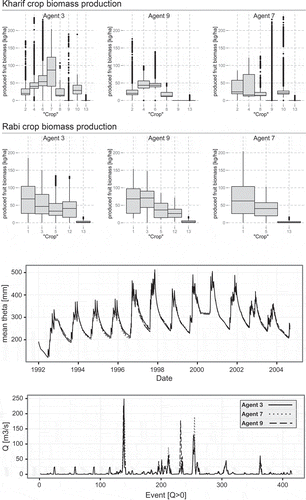
However, the middle and lower panels of Fig. 5 show that the distinctly different cropping realizations have almost no impact on the catchment water balance. Simulated catchment mean soil moisture and discharge hardly differ among the different strategies. This is a discouraging result as we intended to analyse the environmental impact of different cropping strategies mainly with respect to efficient water harvesting through enlarging soil water storage and to reduce erosion exposure by reducing overland flow.

7 DISCUSSION AND CONCLUSIONS

Although we have tackled many open questions the core of this study is the PUB experiment using eco-hydrological modelling tools to address socio-ecological issues in a data-scarce setting. We structure the first part of the discussion with respect to the hypotheses set out in the pre-analysis (Section 2). The second part details how this experiment contributes to the PUB issue.

7.1 Targeted data assessment and model selection to characterize/represent the dominant landscape elements and processes

A data assessment with a strong focus on the major controllers of Horton overland flow in the selected model (infiltration capacity, hydraulic conductivity, porosity, suction at the wetting front) and spatial structure resulted in a comprehensive dataset that allowed direct application of the WASA_crop map without calibration to observed discharge.

The combination of bottom-up analysis and RS classification according to the spectral signatures of the same first- and second-order characteristics allowed the regionalization of the functional soil profiles identified within the catenas. A spatial verification of the RS classification scheme with roughly 20% significant misfits for both soil and land-use characteristics was found to be acceptable.

Uncalibrated predictions with WASA_crop produced a reasonable match of the seasonal water balance and daily discharge dynamics, except in seasons 3 and 5 when observed seasonal runoff coefficients appear to be unrealistically high. This was mainly achieved through a reasonable representation of the overland flow generation and the spatial organization of the landscape entities. Moreover, the spatial pattern of topsoil moisture by WASA_crop appears plausible when compared to distributed soil moisture proxies. This was a prerequisite for the extension of the model by a crop subroutine.

The comparison to model runs without the full dataset undermines the importance of the structural information that has been collected with the proposed sampling strategy. While WASA_zero performs poorly when parameterized based on the broad soil and geological maps (using the same semi-automated delineation algorithm LUMP; Francke et al. 2008), exchanging the precise but scarce hydraulic soil parameters with standard values after Carsel and Parrish (1988) in the fully parameterized model has a minor impact (Fig. 3). Hence, the spatial mapping of land use and the major functional soil types and depth appear to provide more substantial insight than additional, precise soil-hydraulic parameter investigations.

We thus conclude that hypothesis H1—the catena is a first-order control—is corroborated by the presented findings. Also, hypothesis H2—that our sampling strategy is feasible—is validated. From the model analysis with different levels of information in Section 6.3 we can additionally infer, that for the given scale and regime, the distributed soil data are of greater importance than a precise and statistically robust sampling of van Genuchten-Mualem parameters.

Thus, the idea to (a) characterize the key landscape elements with respect to the key model parameters and their patterns as well as possible, and (b) regionalize these model parameters (here functional soil profiles) to all members in a soil class based on similar spectral properties, seems to a certain extent a feasible approach. The Landsat data, despite their drawbacks, were valuable as moderately spatially-resolved information for this mesoscale application, reflecting the same findings of Montzka et al. (2008). As a PUB experiment it is noteworthy that these data are globally available through open access technology.

We admit that the idea of focusing on the dominant landscape elements and the catena is not new. Hellebrand et al. (2011) presented a dominant runoff process approach for 15 European basins. Zehe et al. (2001) employed the approach to characterize the Weiherbach (a Horton landscape in a humid region) and set up a catchment model that allowed successful prediction of the rainfall–runoff dynamics. Similar to the present case, baseflow dynamics were of minor importance. Blume et al. (2008, 2009) successfully applied the same approach in a very humid catchment in Chile, where subsurface flow was the dominant process. Note that the Mod catchment is two orders of magnitude larger than the two latter catchments and that the money and time available for this study were much smaller. Also, non-process based approaches acknowledge the importance of landscape structure, e.g. SWAT enhanced landscape unit discretization (Arnold et al. 2010).

We can state that hypothesis H3 (that WASA_crop is a suitable model structure for describing the dominant processes and that the performance of an uncalibrated simulation is an excellent benchmark to test the feasibility of the assessment and regionalization of functional soil data) is to a large extent corroborated by the presented findings. Thus the approach is one possible alternative to, for example, Monte Carlo simulations with HBV-type models under similar conditions (Love et al. 2010).

Nevertheless, we are well aware of the limitations of the derived functional soil map in capturing spatial variability and the uncertainty of key parameters due to the small number of unsophisticated infiltration experiments and the very small number of undisturbed soil samples. In addition, it would be desirable to have integral measures of hydrological behaviour, such as sediment fingerprinting (Martínez-Carreras et al. 2010) to characterize the source area of overland flow, or distributed soil moisture data (Brocca et al. 2007, Zehe et al. 2010) to verify the simulated soil moisture dynamics against either distributed point data or spatially clustered data. Further, use of a larger number of reference catenas would be advantageous. However, our data assessment was accomplished within a reasonable amount of time (10 person-weeks of field investigation) and using either low-tech instruments or freely available data sources, which are also available for researchers at local colleges. We think this aspect is particularly relevant for PUB, as scientists in many ungauged basins may be unable to buy high-tech equipment or expensive satellite products.

7.2 No feedbacks in a fully coupled eco-hydrological model?

The presented results show clearly that hypothesis H4—which is crucial for the proposed land-use strategy analysis—is wrong. The fully coupled WASA_crop did not produce strong feedbacks of different biomass production on the soil moisture dynamics. Our idea was that water stress affects crop growth and dynamics of leaf area index, stand height and root depth, which in turn impact on interception, water uptake and (evapo-)transpiration, which then feedback on soil moisture dynamics, infiltration capacity and overland flow and vice versa.

WASA uses Green-Ampt to describe infiltration instead of the more complex Richards equation. The speed of the infiltration front is thus controlled by saturated hydraulic conductivity (k_s, which is constant) and suction at the wetting front. Given the high rainfall intensities during the monsoon season, a small increase in the suction due to less soil moisture has a strong effect on infiltration velocity, which controls the formation of infiltration excess overland flow. Were the the Richards equation to be used, lower soil moisture would also result in drastically reduced unsaturated hydraulic conductivity. In the case of fine-grained soils, effect often dominates against increasing potential gradients (Zehe and Blöschl 2004, Zehe et al. 2007).

However, the sensitivity bands of the hydrological and the crop model do not fully overlap. This raises a fundamental question about the model coupling as we have already integrated specifically suitable and proven submodels. Although not part of this study, an analysis of SWAP in comparison to crop yield and lysimeter hydrology points to issues of parameter interaction for crop and soil that cannot be calibrated separately. A brief summary is given in the Appendix. Hence we propose caution when coupling ready-developed models if the main target is to account for bi-directional feedbacks. This was also found by Tietjen and Jeltsch (2007) for grazing landscapes, who then developed the Ecohyd model (Tietjen et al. 2009, 2010).

7.3 Data limitations and scale

When discussing parsimonious data assessment we clearly have to look at which data are most scarce or needed. Much less distributed information and coarser models may only suffice to represent the mean behaviour if we can build on better runoff data—the integral response of the catchment. However, the PUB situation strongly restricts the applicability of such approaches (He et al. 2011) as they need at least some gauge information.

PUB is not merely dealing with a missing node in a dense observation network. Nor is it limited to discharge data. It challenges model and data needs. We have shown that the identification of dominant processes and first-order controls—in our case Horton overland flow generation (infiltration capacity and rainfall intensity), and its spatial organization along catenas (topographic gradients, roughness and re-infiltration)—is of great importance for characterizing the system. Providing spatially-distributed information to the model alone greatly improves the model performance. Our hierarchical approach identified and characterized the major landscape elements, while their spatial distribution was derived from RS analyses. Thus matching the ‘pattern’ organizing the dominant processes is suggested as being more important than precise van Genuchten-Mualem parameters in our case. It is a method that balances the need for sufficiently accurate characterization of soil properties and their relative differences along the hillslope catena. This holds because we need to characterize several thousand catenas at this scale.

With respect to the spatial variability of parameters, we clearly have to point out that using so few samples generally lacks statistical robustness. We may not even capture the whole spectrum of properties. However, the overall variability and its spatial distribution are already captured by the RS analyses. Hence, under the strong constraints of addressing data-scarce regions, our approach is encouraging because it tackles the issue from two sides:

1. The general spectrum of properties, heterogeneity and topology are handled top-down. Thus we identify functional classes independently but based on the same characteristics as the bottom-up derivation of their respective properties based on representative samples. Thus we derive a concise data basis from analyses at the appropriate scales.

2. There is a clear focus on the dominating processes. This refers to the data required for the analysis and the model. The greatest data limitation in our case is discharge data—this cannot be changed in a single measurement campaign. Second come infiltration capacity and topography as the most crucial properties for representing the Horton landscape. Both have been addressed with high priority. In contrast, soil water retention parameters α and n are found to be less important and show much lower variability and sensitivity. Thus we are confident with the five samples we analysed for these properties.

7.4 Lessons from the PUB experiment for the PUB problem

To conclude, we have shown that our approach is feasible through its awareness of scale, processes and model concepts. The combination of a distributed model suitable for the landscape and the data assessment strategy focusing on structural information and relative differences, made this PUB experiment successful. Regarding its transferability, we again emphasize the close interrelation of the three aspects, which has been broadly discussed since Klemeš (1983). A different representation or a different target property would require different data. The same holds for different regimes with different dominating processes and different effective scales. However, PUB is more than the problem of a missing gauge or the difficulties arising with complex systems. Our experiment tried to deal with these in many respects, while aiming for distributed soil moisture and crop production predictions. Although it could be improved with regard to many details, the general concept is found suitable for data-scarce places, especially if there is limited budget for equipment and staffing, as in many PUB settings.

Process-based, spatially-explicit models such as WASA, which allow uncalibrated simulations based on estimated but distributed observable soil and vegetation characteristics, are valuable and useful tools for PUB hydrology at the mesoscale. The results presented are certainly insufficient to dispel all valid scepticism regarding the used methods and approximations. However, the general approach in combination with the developed targeted data assessment strategies, is suitable for PUB.

Full coupling of well-established models does not assure that they produce the right feedbacks, even if they appear well suited for this issue. This may not be too relevant for PUB issues, but is certainly pertinent to the issue of integrated modelling. To account for bi-directional feedbacks, generic model development specific to the problem may be much better than coupling existing models without thorough analysis of their sensitivity bands and parameter interaction.

A next generalizing step to a procedure for approaching ungauged catchments could involve the following four aspects:

1. A more flexible integration of dominating processes and model representations similar to ‘Superflex’ (Fenicia et al. 2011) and ‘the method of multiple working hypotheses’ (Clark et al. 2011). In contrast to the approaches proposed above, these rely on spatially-distributed parameters. Such calibration and regionalization procedures would require a completely different workflow.

2. A functional description of hydrologic units and processes to link observable properties, with concepts and parameters, as proposed by the current DFG Research Group ‘From Catchments as Organized Systems to Models based on Functional Units’. Because PUB still challenges today’s hydrology, we believe that we have to question the methodology and reverse the standard approach.

3. An advanced understanding of, and a methodology for, information content analysis of diffent data and model conceptualizations as argued by Gupta et al. (2012).

4. Substantial progress in understanding of the soil–water–atmosphere–plant system and eco-hydrological feedbacks in general. That it is reasonable to generically develop models for specific feedbacks was shown by Tietjen et al. (2007, 2009, 2010). New approaches based on self-optimization and dynamic adaptation are opened up by Kleidon (2007) and Schymanski et al. (2009).

Funding

The project was sustained through the reliable scholarship of the Heinrich Böll Foundation and the German Academic Foundation, which are gratefully acknowledged.

SUPPLEMENTARY MATERIAL

The underlying research materials for this article can be requested from the corresponding author [email protected]

Acknowledgements

We wish to express our gratitude to all the people in Jhabua who helped during the fieldwork and research for data. The study benefited greatly from the generous resourcing of laboratory facilities and data at the College of Agriculture, Jawaharlal Nehru Krishi Vishwavidyalaya, Indore. Anke Hildebrandt contributed much to the study in the Appendix. Moreover, we thank the anonymous reviewers for their help in substantially improving our article.

APPENDIX

ANALYSIS OF PARAMETER INTERACTION OF SWAP

Motivated by the preceding model applications and the failure of hypothesis H4, we tested SWAP (Kroes and van Dam 2003) against lysimeter data. We collected data from the Lysimeter Station Brandis, in Germany, where natural soil cores (3 m³) from four different locations with three replications are monitored under identical cropping and weather conditions.

Methods and set-up

The observations show that soil does have a strong influence on the yield produced. In order to analyse the regionalizability of parameters (Hundecha and Bardossy 2004, Samaniego et al. 2010), we incorporated SWAP into an automatic Dynamically Dimensioned Search (DDS) calibration algorithm (Tolson and Shoemaker 2007). Starting from measured values, 15 000 iterations were allowed to vary seven soil-specific parameters for each layer and seven crop-specific parameters within predefined acceptable ranges. The parameters were selected based on Pauwels et al. (2007) and Kroes and van Dam (2003), and by comparison with different standard crop parameter sets from earlier WOFOST applications (de Wit and van Diepen 2007). The dataset was reduced to years cropped with winter wheat.

To examine the dependency between the crop and soil parameters we set up several calibration and validation schemes. Figure A1 presents four settings: A employs the model as a tool with physically meaningful parameters, where all inputs are derived from measurements and observations; B describes a succeeding calibration of soil and crop parameters (to avoid the influence of vegetation cover on the soil water dynamics and snow, the soil parameters were calibrated in warm winters only; using the calibrated soil parameters, the crop parameters were calibrated by running the model over the whole growing season); C stands for the joint calibration of crop and soil parameters over the whole growing season; and X is a cross-validation of the parameter sets found for the winter wheat crop on each lysimeter to all other lysimeters.

Fig. A1 SWAP analysis calibration schemes.

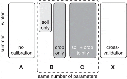
Results

The calibration study assesses the SWAP model’s capability to represent crop development, soil water dynamics and their interactions. An overview of the validation results is given in Fig. A2, where observed vs modelled crop dry matter is plotted for each lysimeter with parameters derived from the respective calibration scheme, A–C. The lysimeters are grouped into soil types. The calibration of soil parameters and, more effectively, the joint calibration of soil and crop parameters improve the capability to project yields on specific soils. Although the influence of soil on yield is somehow represented, variance remains rather high.

Fig. A2 Overview about SWAP validation results after the respective calibration schemes A–C.

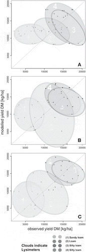
A close-up of the soil moisture dynamics at two example lysimeters indicates persistant difficulties in the representation of crop–soil interactions. Figure A3 shows the validation crop model run for the 1996/97 winter wheat growing season by presenting the absolute water content in the lysimeter. In addition, the box plots in the right panel present the performance of all validation years for all lysimeters with respect to the water balance (R²). The dashed (red) line marks the mean of all realizations within the specific calibration scheme. Although we allow the same parameter space for calibration schemes B and C, a joint calibration also yields better results for the water balance. Calibration of the soil alone produces poor results.

Fig. A3 Comparison of observed and modelled soil moisture dynamics at lysimeter 10_3 (Loess Chernozem Silt Loam) and 7_5 (Cambisol/Stagnosol Loam) as time series from 01-08-1996 with daily time step. Standard refers to a standard parameterization without calibration. Right panel: The box plots present the performance of all validation years for all lysimeters with respect to water balance (R²). The dashed (red) line marks the mean of all realizations within the specific calibration scheme.

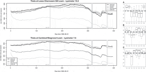
Thus far we have retained the soil–crop combination of each lysimeter in the validation. But the model is meant and used for several locations where no specific crop calibration is possible. Moreover, the physical description of the soil water balance should allow at least some transferability. When applying the calibrated crop parameters to calibrated soil parameters of other lysimeters, the result can no longer be validated; Fig. A4 presents the observed against modelled total dry matter yield.

Fig. A4 Cross-validation of yield simulation with SWAP using calibrations of the same crop to different soils.

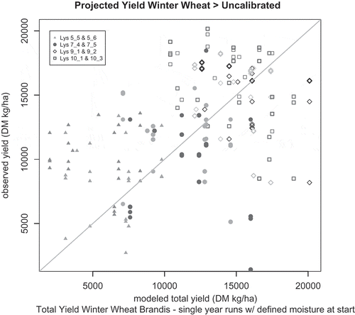
Conclusion

Notwithstanding the physical description of the parameters, the SWAP model needs specific calibration for soil and crop. The parameter sets are poorly transferable.

REFERENCES

- Abbott, M., et al., 1986. An introduction to the European hydrological system – Système Hydrologique Européen, “SHE,” 1: history and philosophy of a physically-based, distributed modelling system. Journal of Hydrology, 87 (1–2), 45–59. doi:10.1016/0022-1694(86)90114-9.
- Abrahamsen, P. and Hansen, S., 2000. Daisy: an open soil–crop–atmosphere system model. Environmental Modelling and Software with Environment Data News, 15 (3), 313–330. doi:10.1016/S1364-8152(00)00003-7.
- Arnold, J.G., et al., 2010. Assessment of different representations of spatial variability on SWAT model performance. Transactions of the ASABE, 53 (5), 1433–1443. doi:10.13031/2013.34913.
- Arnold, J.G., et al., 2012. SWAT: model use, calibration, and validation. Transactions of the ASABE, 55 (4), 1491–1508. doi:10.13031/2013.42256.
- Baumgardner, M.F., Silvall, L.F., and Biehll, L.L., 1985. Reflectance properties of soils. Advances in Agronomy, 38. doi:10.1016/S0065–2113(08)60672–0.
- Beven, K., 1989. Changing ideas in hydrology — the case of physically-based models. Journal of Hydrology, 105 (1–2), 157–172. doi:10.1016/0022-1694(89)90101-7.
- Beven, K., 2000. Uniqueness of place and process representations in hydrological modelling. Hydrology and Earth System Sciences, 4 (2), 203–213.
- Beven, K., 2006. Searching for the Holy Grail of scientific hydrology: Qt = H(S, R, ∆t)A as closure. Hydrology and Earth System Sciences, 10 (5), 609–618.
- Beven, K. and Kirkby, M., 1979. A physically based, variable contributing area model of basin hydrology. Hydrological Sciences Bulletin, 24 (1), 43–69. doi:10.1080/02626667909491834.
- Blöschl, G., et al., eds., 2013. Runoff predictions in ungauged basins – synthesis across processes, places and scales. Cambridge University Press. Available from: http://www.cambridge.org/9781107028180.
- Blume, T., Zehe, E., and Bronstert, A., 2009. Use of soil moisture dynamics and patterns at different spatio-temporal scales for the investigation of subsurface flow processes. Hydrology and Earth System Sciences, 13 (7), 1215–1233.
- Blume, T., et al., 2008. Investigation of runoff generation in a pristine, poorly gauged catchment in the Chilean Andes I: a multi-method experimental study. Hydrological Processes, 22, 3661–3675. doi:10.1002/hyp.6971.
- Bonhomme, R., 2000. Bases and limits to using ‘degree day’ units. European Journal of Agronomy, 13, 1–10. doi:10.1016/S1161-0301(00)00058-7.
- Boogaard, H., et al., 1998. WOFOST 7.1 - User’s guide for the WOFOST 7.1 crop growth simulation model and WOFOST Control Center 1.5. Wageningen: Alterra WUR.
- Bouman, B.A.M., et al., 1996. The “School of de Wit” crop growth simulation models: a pedigree and historical overview. Agricultural Systems, 52, 171–198. doi:10.1016/0308-521X(96)00011-X.
- Brocca, L., et al., 2007. Soil moisture spatial variability in experimental areas of central Italy. Journal of Hydrology, 333 (2–4), 356–373. doi:10.1016/j.jhydrol.2006.09.004.
- Carsel, R.F. and Parrish, R.S., 1988. Developing joint probability distributions of soil water retention characteristics. Water Resources Research, 24 (5), 755–769. AGU. doi:10.1029/WR024i005p00755.
- Chuanyana, Z., Zhongrena, N., and Zhaodong, F., 2004. GIS-assisted spatially distributed modeling of the potential evapotranspiration in semi-arid climate of the Chinese Loess Plateau. Journal of Arid Environments, 58, 387–403. doi:10.1016/j.jaridenv.2003.08.008.
- Clark, M., Kavetski, D., and Fenicia, F., 2011. Pursuing the method of multiple working hypotheses for hydrological modeling. Water Resources Research, 47 (9), W09301. doi:10.1029/2010WR009827.
- de Wit, A.M. and van Diepen, C.A., 2007. Crop model data assimilation with the Ensemble Kalman filter for improving regional crop yield forecasts. Agricultural and Forest Meteorology, 146, 38–56. doi:10.1016/j.agrformet.2007.05.004.
- Dooge, J., 1986. Looking for hydrologic laws. Water Resources Research, 22 (9S), 46S–58S. doi:10.1029/WR022i09Sp0046S.
- Droogers, P. and Allen, R.G., 2002. Estimating reference evapotranspiration under inaccurate data conditions. Irrigation and Drainage Systems, 16, 33–45. doi:10.1023/A:1015508322413.
- Fenicia, F., Kavetski, D., and Savenije, H.H.G., 2011. Elements of a flexible approach for conceptual hydrological modeling: 1. Motivation and theoretical development. Water Resources Research, 47 (11), W11510. doi:10.1029/2010WR010174.
- Francke, T., et al., 2008. Automated catena‐based discretization of landscapes for the derivation of hydrological modelling units. International Journal of Geographical Information Science, 22 (2), 111–132. doi:10.1080/13658810701300873.
- Franke, G., 1994. Nutzpflanzen der Tropen und Subtropen, Vol. 1. Stuttgart: UTB.
- Goldshleger, N., et al., 2004. Soil reflectance as a tool for assessing physical crust arrangement of four typical soils in Israel. Soil Science, 169 (10), 677–687. doi:10.1097/01.ss.0000146024.61559.e2.
- Goudriaan, J. and Van Laar, H.H., 1994. Modelling potential crop growth processes. Dordrecht: Springer, 126. doi:10.1007/978-94-011-0750-1.
- GSI, 1976. Geology and Mineral Resources of the States of India — Part XI. Madhya Pradesh: Geological Survey of India.
- GSI, 1988. District Resource Map — Jhabua District. Madhya Pradesh: Geological Survey of India.
- Güntner, A. and Bronstert, A., 2004. Representation of landscape variability and lateral redistribution processes for large-scale hydrological modelling in semi-arid areas. Journal of Hydrology, 297 (1–4), 136–161. doi:10.1016/j.jhydrol.2004.04.008.
- Güntner, A., et al., 2004. Simple water balance modelling of surface reservoir systems in a large data-scarce semiarid region. Hydrological Sciences Journal, 49 (5), 901–918. doi:10.1623/hysj.49.5.901.55139.
- Gupta, H., et al., 2012. Towards a comprehensive assessment of model structural adequacy. Water Resources Research, 48 (8), 1–40. doi:10.1029/2011WR011044.
- He, Y., Bárdossy, A., and Zehe, E., 2011. A review of regionalisation for continuous streamflow simulation. Hydrology and Earth System Sciences, 15 (11), 3539–3553. doi:10.5194/hess-15-3539-2011.
- Hellebrand, H., et al., 2011. A process proof test for model concepts: modelling the meso-scale. Physics and Chemistry of the Earth, Parts A/B/C, 36 (1–4), 42–53. doi:10.1016/j.pce.2010.07.019.
- Hundecha, Y. and Bárdossy, A., 2004. Modeling of the effect of land use changes on the runoff generation of a river basin through parameter regionalization of a watershed model. Journal of Hydrology, 292 (1–4), 281–295. doi:10.1016/j.jhydrol.2004.01.002.
- Ittersum, M.V., et al., 2003. On approaches and applications of the Wageningen crop models. European Journal of Agronomy, 18, 201–234. doi:10.1016/S1161-0301(02)00106-5.
- Jackson, R., Jobbágy, E., and Nosetto, M., 2009. Ecohydrology in a human-dominated landscape. Ecohydrology, 2 (3), 383–389. doi:10.1002/eco.81.
- Keshavamurty, R. and Rao, M.S., 1992. The physics of monsoons. New Delhi: Allied Publishers.
- Kleidon, A., 2007. Thermodynamics and environmental constraints make the biosphere predictable — a response to Volk. Climatic Change, 85, 259–266. doi:10.1007/s10584-007-9320-x.
- Klemeš, V., 1983. Conceptualization and scale in hydrology. Journal of Hydrology, 65, 1–23. doi:10.1016/0022-1694(83)90208-1.
- Kroes, J. and van Dam, J., 2003. Reference Manual SWAP version 3.0.3.
- Krysanova, V., Hattermann, F., and Wechsung, F., 2005. Development of the ecohydrological model SWIM for regional impact studies and vulnerability assessment. Hydrological Processes, 19 (3), 763–783. doi:10.1002/hyp.5619.
- Kucharik, C.J. and Brye, K.R., 2003. Integrated BIosphere Simulator (IBIS) yield and nitrate loss predictions for Wisconsin maize receiving varied amounts of nitrogen fertilizer. Journal of Environment Quality. 32 (1), 247–268. doi:10.2134/jeq2003.2470.
- Lei, H., et al., 2008. Modeling the crop transpiration using an optimality-based approach. Science in China Series E: Technological Sciences, 51, 60–75. doi:10.1007/s11431-008-6008-z.
- Lindström, G., et al., 1997. Development and test of the distributed HBV-96 hydrological model. Journal of Hydrology, 201 (1–4), 272–288. doi:10.1016/S0022-1694(97)00041-3.
- Love, D., et al., 2010. Rainfall–interception–evaporation–runoff relationships in a semi-arid catchment, northern Limpopo basin, Zimbabwe. Hydrological Sciences Journal, 55 (5), 687–703. doi:10.1080/02626667.2010.494010.
- Martínez-Carreras, N., et al., 2010. A rapid spectral-reflectance-based fingerprinting approach for documenting suspended sediment sources during storm runoff events. Journal of Soils and Sediments, 10 (3), 400–413. doi:10.1007/s11368-009-0162-1.
- Mayor, Á., Bautista, S., and Bellot, J., 2009. Factors and interactions controlling infiltration, runoff, and soil loss at the microscale in a patchy Mediterranean semiarid landscape. Earth Surface Processes and Landforms, 34 (12), 1702–1711. doi:10.1002/esp.1875.
- McDonnell, J., et al., 2007. Moving beyond heterogeneity and process complexity: a new vision for watershed hydrology. Water Resources Research, 43, doi:10.1029/2006WR005467.
- Montzka, C., et al., 2008. Modelling the water balance of a mesoscale catchment basin using remotely sensed land cover data. Journal of Hydrology, 353 (3–4), 322–334. doi:10.1016/j.jhydrol.2008.02.018.
- Mueller, E., et al., 2009. Modelling the effects of land-use change on runoff and sediment yield for a meso-scale catchment in the Southern Pyrenees. CATENA, 79 (3), 288–296. doi:10.1016/j.catena.2009.06.007.
- Mueller, E.N., Wainwright, J., and Parsons, A.J., 2007. Impact of connectivity on the modeling of overland flow within semiarid shrubland environments. Water Resources Research, 43, (9). doi:10.1029/2006WR005006.
- Norman, M., Pearson, C., and Searle, P., 1995. The ecology of tropical food crops, Vol. 1. Cambridge University Press.
- Parajka, J., Merz, R., and Blöschl, G., 2005. A comparison of regionalisation methods for catchment model parameters. Hydrology and Earth System Sciences, 9 (3), 157–171. doi:10.5194/hess-9-157-2005.
- Pauwels, V.R.N., et al., 2007. Optimization of a coupled hydrology-crop growth model through the assimilation of observed soil moisture and leaf area index values using an ensemble Kalman filter. Water Resources Research, 43, (4). doi:10.1029/2006WR004942.
- Pilgrim, D., Chapman, T., and Doran, D., 1988. Problems of rainfall–runoff modelling in arid and semiarid regions. Hydrological Sciences Journal, 33 (4), 379–400. doi:10.1080/02626668809491261.
- Rehm, S. and Espig, G. 1991. The cultivated plants of the tropics and subtropics. Champaign, IL: Balogh Scientific Books.
- Renard, K., et al., 2008. A brief background on the US Department of Agriculture Agricultural Research Service Walnut Gulch Experimental Watershed. Water Resources Research, 44 (5), W05S02. doi:10.1029/2006WR005691.
- Rodriguez-Iturbe, I., 2000. Ecohydrology: a hydrologic perspective of climate-soil-vegetation dynamies. Water Resources Research, 36 (1), 3–9. doi:10.1029/1999WR900210.
- Rodriguez-Iturbe, I., et al., 1999. On the spatial and temporal links between vegetation, climate, and soil moisture. Water Resources Research, 35, 3709–3722. doi:10.1029/1999WR900255.
- Samaniego, L., Kumar, R., and Attinger, S., 2010. Multiscale parameter regionalization of a grid-based hydrologic model at the mesoscale. Water Resources Research, 46 (5), W05523. doi:10.1029/2008WR007327.
- Schaap, M.G., Leij, F.J., and van Genuchten, M.T., 2001. Rosetta: a computer program for estimating soil hydraulic parameters with hierarchical pedotransfer functions. Journal of Hydrology, 251 (3–4), 163–176. doi:10.1016/S0022–1694(01)00466–8.
- Schulla, J. and Jasper, K., 2007. Model description WaSiM-ETH. Technical report. Zürich: ETH Zürich.
- Schymanski, S., et al., 2009. An optimality-based model of the dynamic feedbacks between natural vegetation and the water balance. Water Resources Research, 45. doi:10.1029/2008WR006841.
- Schymanski, S.J., 2008. Optimality as a concept to understand and model vegetation at different scales. Geography Compass, 2 (5), 1580–1598. doi:10.1111/j.1749-8198.2008.00137.x.
- Shuttleworth, W. and Wallace, J., 2007. Evaporation from sparse crops-an energy combination theory. Quarterly Journal of the Royal Meteorological Society, 111 (469), 839–855. doi:10.1002/qj.49711146910.
- Simunek, J., van Genuchten, M., and Sejna, M., 2008. Development and applications of the HYDRUS and STANMOD software packages and related codes. Vadose Zone Journal, 7 (2), 587–600. doi:10.2136/vzj2007.0077.
- Singh, A.K., 2004. Towards decision support models for an ungauged catchment in India, the case of Anas catchment. Mitteilungen des Instituts für Wasserwirtschaft und Kulturtechnik der Universität Karlsruhe (TH), 225.
- Sivapalan, M., et al., 2003. IAHS Decade on Predictions in Ungauged Basins (PUB), 2003–2012: shaping an exciting future for the hydrological sciences. Hydrological Sciences Journal, 48 (6), 857–880. doi:10.1623/hysj.48.6.857.51421.
- Stull, R.B., 2001. An introduction to boundary layer meteorology. Berlin: Springer.
- Tian, F., et al., 2006. Extension of the representative elementary watershed approach for cold regions via explicit treatment of energy related processes. Hydrology and Earth System Sciences, 10 (5), 619–644. doi:10.5194/hess-10-619-2006.
- Tietjen, B., et al., 2010. Effects of climate change on the coupled dynamics of water and vegetation in drylands. Ecohydrology, 3, 226–237. doi:10.1002/eco.70.
- Tietjen, B. and Jeltsch, F., 2007. Semi-arid grazing systems and climate change: a survey of present modelling potential and future needs. Journal of Applied Ecology, 44 (2), 425–434. doi:10.1111/j.1365-2664.2007.01280.x.
- Tietjen, B., Zehe, E., and Jeltsch, F., 2009. Simulating plant water availability in dry lands under climate change: a generic model of two soil layers. Water Resources Research, 45. doi:10.1029/2007WR006589.
- Tolson, B. and Shoemaker, C., 2007. Dynamically dimensioned search algorithm for computationally efficient watershed model calibration. Water Resources Research, 43 (1), W01413. doi:10.1029/2005WR004723.
- Tomar, V., Gupta, G., and Kaushal, G., 1995. Soil resources and agroclimatic zones of Madhya Pradesh.
- Tsuji, G.Y., Hoogenboom, G., and Thornton, P.K. 1998. Understanding options for agricultural production. Dordrecht: Kluwer Academic Press.
- Ustin, S., ed., 2004. Manual of remote sensing, remote sensing for natural resource management and environmental monitoring, Vol. 4. Hoboken, NJ: Wiley.
- van Dam, J.C. and Malik, R.S., 2003. Water productivity of irrigated crops in Sirsa district, India. Technical Report by WUR. Wageningen: WUR.
- van Dam, J.C., et al., 2008. Advances of modeling water flow in variably saturated soils with SWAP. Vadose Zone Journal, 7 (2), 640–653. doi:10.2136/vzj2007.0060.
- Xavier, A.C. and Vettorazzi, C.A., 2004. Monitoring leaf area index at watershed level through NDVI from Landsat-7/ETM+ data. Scientia Agricola, 61, 243–252. scielo. doi:10.1590/S0103-90162004000300001.
- Yadav, M., Wagener, T., and Gupta, H., 2007. Regionalization of constraints on expected watershed response behavior for improved predictions in ungauged basins. Advances in Water Resources, 30 (8), 1756–1774. doi:10.1016/j.advwatres.2007.01.005.
- Yatheendradas, S., et al., 2008. Understanding uncertainty in distributed flash flood forecasting for semiarid regions. Water Resources Research, 44 (5), W05S19. doi:10.1029/2007WR005940.
- Zehe, E. and Blöschl, G., 2004. Predictability of hydrologic response at the plot and catchment scales: role of initial conditions. Water Resources Research, 40 (10). doi:10.1029/2003WR002869.
- Zehe, E. and Sivapalan, M., 2009. Threshold behaviour in hydrological systems as (human) geo-ecosystems: manifestations, controls, implications. Hydrology and Earth System Sciences, 13 (7), 1273–1297.
- Zehe, E., et al., 2001. Modeling water flow and mass transport in a loess catchment. Physics and Chemistry of the Earth, Part B: Hydrology, Oceans and Atmosphere, 26 (7–8), 487–507. doi:10.1016/S1464-1909(01)00041-7.
- Zehe, E., et al., 2007. Patterns of predictability in hydrological threshold systems. Water Resources Research, 43, (7). doi:10.1029/2006WR005589.
- Zehe, E., et al., 2010. Plot and field scale soil moisture dynamics and subsurface wetness control on runoff generation in a headwater in the Ore Mountains. Hydrology and Earth System Sciences, 14 (6), 873–889. doi:10.5194/hess-14-873-2010.