Quantifying the impact of urban area expansion on groundwater recharge and surface runoff

ABSTRACT

In this surface water modelling study, a new spatial evaluation for assessing the impact of urbanization was applied for the semi-arid watersheds intersecting with the Gaza coastal aquifer. The SWAT model was calibrated and validated in a semi-automated approach for streamflow in the main watersheds. The results show that the model could simulate water budget components adequately within the complex semi-arid watersheds. Linear relationships between the change in urban area and the corresponding change in surface runoff or percolation were concluded for the urbanized sub-basins. The urban-surface runoff index (USI) and the urban-percolation index (UPI) were developed to represent a micro-level evaluation of different urban change scenarios in the sub-basins. The global urban-surface runoff index (GUSI) and the global urban-percolation index (GUPI) were derived as macro-level factors reflecting the influence on the overall Gaza coastal aquifer due to urban area expansion.

Editor D. Koutsoyiannis Associate editor E. Rozos

KEYWORDS:

• urban change
• spatial response
• SWAT simulation
• sensitivity analysis
• percolation index
• surface runoff index

1 Introduction

Water is the most important natural resource, especially in the arid or semi-arid zones that face high population growth, scarcity of freshwater, irregularity of rainfall, excessive land-use change and increasing vulnerability to risks such as drought, desertification and pollution (Fadil et al. 2011). Assessing the impact of land-use change on hydrological parameters is considered an important step in water resources management and a prerequisite for ecological restoration as well as for their sustainable management. Quantitative evaluation of the impacts of human activities on water resources at watershed level is within the focus of the present research in hydrology (Chu et al. 2010). The spatial approach of quantifying the impact of land-use change at the spatial level of hydrological response units (HRUs) contributes to the understanding of the variation of hydrologic attributes in a basin and its sensitivity; especially, land-use changes towards urban areas influence the water balance. In this study, based on surface water modelling, a new spatial evaluation for assessing the impact of urbanization was applied to the semi-arid watersheds intersecting with the Gaza Strip and the Gaza coastal aquifer.

In 2010, the estimated total population in the Gaza Strip was 1.64 million (Rahman et al. 2013). The area covers 365 km², making it one of the most densely populated regions (approx. 4500 inhabitants/km²) in the world (PCBS 2006). The Gaza Strip faces serious water crises (CMWU 2010). The groundwater aquifer is considered the main water supply source for all kinds of human use (domestic, agricultural and industrial), and can basically only be fed by rainfall and lateral aquifer flow from the east (CMWU 2010). The impervious areas resulting from urban expansion pose a threat to the sustainability of the Gaza coastal aquifer in terms of aquifer replenishment.

In contrast to the number of groundwater studies, considerably less research with regard to surface water has been undertaken in the Gaza Strip. Some of these studies focused on the Gaza boundary and neglected the natural extent of the watersheds through historical Palestine, and were without calibration for model parameters. Other studies estimated the groundwater recharge without considering the spatial dimension. Laronne et al. (2004) studied the characterization and utilization of surface water in the Near East, respectively exemplified by Wadi Gaza and Wadi Samoa reservoirs in historical Palestine. Khalaf et al. (2006) assessed the rainwater runoff based on the proposed regional plan for the Gaza Strip applying a rational method for runoff calculations, Horton’s equation for estimating infiltration, and the geographical information system (GIS) as an analytical tool. Hamdan et al. (2007) applied the rational runoff formula using GIS as a tool to estimate runoff amounts from different land-use categories. Aish et al. (2010) used the WetSpass model, which is integrated within GIS ArcView, to evaluate groundwater recharge in the Gaza Strip. Ajjur and Mogheir (2012) evaluated the effect of climate change on groundwater in the Gaza Strip and studied the temporal relation between rainfall and recharge in three locations. Hamad et al. (2012) evaluated three different urbanization scenarios using the Automated Geospatial Watershed Assessment (AGWA) tool, which works under the umbrella of GIS.

The SWAT (Soil and Water Assessment Tool) model is used in different semi-arid regions to simulate water budget, sediment yield and nutrient transport (SWAT 2013). It is a flexible model that can be used under a wide range of different environmental conditions (Zhang 2005). Recently, SWAT has been widely used in assessing land-use change at different levels. Wang et al. (2013) applied the model for analysing individual and combined impacts of land-use/cover (LULC) and climate change on hydrological processes in a coastal watershed in Alabama, USA. Kim et al. (2013) employed the SWAT model to backcast long-term hydrologic behaviour of watersheds in North Carolina with different land-use/cover conditions. Dong et al. (2013) used long-term observational data as a basis for examining the effects of human activities and climate change on the runoff variation of Jinghe River Basin, a typical arid inland basin in northwest China. Karcher et al. (2013) proposed a modification to the SWAT model to enable the identification of areas where the implementation of best management practices would likely result in the most significant improvements in terms of downstream water quality. Valdivieso and Sendra (2013) studied SWAT performance although they only had scarce information; the model showed a relatively satisfactory reproduction of the historical record of flows with certain limitations in the calculation of sediment production. Memarian et al. (2014) investigated the impact of LULC on the hydrological conditions of the Hulu Langat basin in Malaysia using the SWAT model. Singh et al. (2014) evaluated the model and the data-driven radial basis neural network (RBNN) model for simulating the sediment load of the Nagwa watershed in India, where soil erosion is a severe problem.

This study is innovative as it considers all watersheds intersecting with the Gaza aquifer domain and also calibrates the SWAT model parameters to quantify the impact of urban area expansion on the coastal aquifer recharge and surface runoff in a spatial approach.

The objectives of this study are (1) calibration and validation of the SWAT model in terms of streamflow for three gauges in the main watersheds intersecting with the Gaza coastal aquifer, and (2) spatial evaluation and quantification of the impact of urban land-use change on percolation and surface runoff at the sub-basin and Gaza coastal aquifer level.

2 Study area

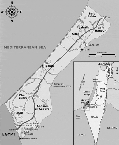
Palestine belongs to the sub-tropical zone. Along the coast (Gaza Strip) and in the highlands (West Bank), the climate is of the Mediterranean type with long, hot and dry summers, and short, cool and rainy winters (Dudeen 2001). The study area forms a transitional zone between the sub-humid coastal zone in the north, the semi-arid loess plains in the northern Negev Desert in the east and the arid Sinai Desert in Egypt in the south (Isaac et al. 2006). The Gaza Strip (Fig. 1) is a narrow coastal strip located on the southeastern coast of the Mediterranean Sea, with a land area covering 365 km², and has a semi-arid climate with a short and mild rainy season and dry summer (CMWU 2010). Although the Gaza Strip and the Israeli side share the biggest surface water basin in historical Palestine (Wadi Gaza basin), the natural flow extent of this basin to the Gaza Strip is cut by Israeli reservoirs. Gaza has a sub-aquifer that is part of the larger coastal aquifer that extends from Karmel Mountain in the north to the Sinai Desert in the south with a variable width and depth (Baaloush 2008). The aquifer domain boundary extends beyond the political boundaries of the Gaza Strip towards the north, towards the east where the coastal aquifer pinches out to the surface, towards the south in Egypt, and finally towards the west to the Mediterranean Sea (HWE 2010).

Figure 1. Gaza Strip.

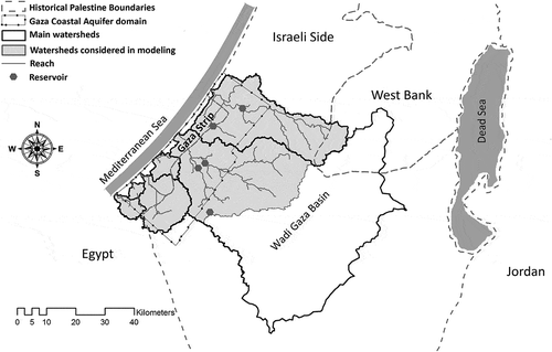
The study area includes the watersheds intersecting with the Gaza Strip as well as the Gaza coastal aquifer domain. The Israeli reservoirs were considered in the watershed delineation, especially in the Wadi Gaza watershed (the largest watershed in historical Palestine). Figure 2 displays the watersheds considered in the modelling process and clarifies that the Wadi Gaza watershed is not totally included in the study area.

Figure 2. Study area.

3 Data and methods

3.1 Data processing

3.1.1 Topography

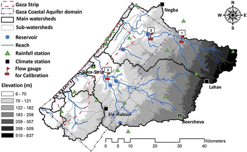
The general topography of the study area ranges from 0 to 840 m elevation. Through 40 km from the west to the east, the elevation gradient is moderate (from 0 to 300 m) and then it becomes steep (from 300 to 840 m) over a distance of less than 10 km. The digital elevation model of the study area (30 m DEM) is shown in Fig. 3 (USGS 2012), and is considered as the basis of the main watershed delineation.

Figure 3. Study area—rainfall, climate, and flow stations and 30-m digital elevation model (DEM).

3.1.2 Climate

The climate of the study area is relatively heterogeneous in terms of rainfall, temperature, solar radiation and evaporation. Table A1 (Appendix A) shows the climate parameters for five stations distributed throughout the study area. Figure 3 depicts the location of these climate stations used in this study. The average annual rainfall (2004–2010) varies from 163 mm in Beersheva to 393 mm in Negba, while Gaza city receives 315 mm. The annual pan evaporation ranges from 1620 mm in Gaza city to 1950 mm in Beersheva, and the mean temperature varies between 8–14°C in January and 21–28°C in August (Meteorological Service database 2013, PWA 2013).

3.1.3 Soil

There are different types of topsoil in the study area, and their spatial distribution was digitized using ArcGIS 10.0 based on the available soil data (Fig. 4; Hamad et al. 2012; Dan et al. 1976). Brown lithosols and loessial arid brown soils occur mainly on steep, rocky and eroded slopes. The underlying rocks may be chalk, marl, limestone or conglomerate, most of which are covered by a hard lime crust. Brown lithosols and loessial serozems occur as shallow brown lithosols with numerous rock outcrops and rendzinic desert lithosols on steep hillslopes and loessial serozems in broad valleys, on terraces and on large plateaux. The underlying rocks are mainly chalk, Nari lime crust, limestone, dolomite and flint. Brown rendzinas soil consists of shallow brown rendzinas with numerous outcrops of limestone or calcareous crust. The underlying rocks are soft chalk and marl covered partly by Nan lime crust. Dark brown soils have developed from fine aeolian sediments, coastal sand calcareous sandstone (kurkar), and medium- to fine-textured alluvial deposits. Loessial serozems developed from loessial sediments, some sandy sediments and gravel. Pararendzinas cover most of the slopes and developed from calcareous sandstone or caicrete that covers this sandstone. Sandy regosols are shallow (0.5–1.5 m) young sandy deposits covering almost the whole landscape. They developed from sand deposits or loessial deposits mixed partly with sand. Regosols cover the steep, eroded slopes and the parent material is sand, clay or loess. Moderate slopes are covered mostly by loessial soils. Mainly these soils developed from loessial sediments: in sandy, eroded areas (in the west) or gravel, conglomerates and chalk (in the east) (Dan et al. 1976). Soil textural classes are listed in Table 1.

Figure 4. Study area—soil types based on Dan et al. (1976) and Ministry of Planning (MoP 2007).

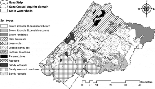
Table 1. Soil texture in the study area.

Soil type	Layer	Hydrologic group^d	Soil textural classes %			Ks *	AWC **	Soil texture
			Clay	Silt	Sand
Brown lithosols & loessial arid brown^a	1	C	20	40	40	13	0.32	Loamy
	2		30	35	35	2.3	0.25	Loam to clay loam
	3		40	30	30	0.6	0.19	Clay loam to clay
Brown lithosols & loessial serozems^a	1	C	15	38	52	26	0.26	Sandy loam to loam
	2		30	35	35	2.3	0.25	Loam to clay loam
Brown rendzinas^a	1	C	35	35	30	2.3	0.18	Clay loam with high granular content
Dark brown soils^b	1	B	25.3	12.8	61.9	4.3	0.18	Sandy loam to sandy clay loam
Loess soils^b	1	A	6	34	58	26	0.2	Sandy loam
Loessial sandy^b	1	A	18	25	57	26	0.2	Sandy loam
Loessial serozems^c	1	C	16	48.8	35.2	13	0.32	Loamy
	2		36	44	20	2.3	0.18	Clay loam
Pararendzinas^a	1	A	4	4	92	210	0.1	Sandy
	2		10	25	65	26	0.2	Sandy loam
Regosols^a	1	A	10	25	65	26	0.2	Sandy loam
Sandy loess^b	1	C	23.2	20.3	56.5	4.3	0.2	Sandy clay loam
Sandy loess soil over loess^b	1	A	17.5	16.3	66.2	26	0.2	Sandy loam
Sandy regosols^b	1	A	8.5	1.8	89.7	210	0.1	Sandy

^aSoil texture: Dan et al. (1976), soil textural classes: FAO (2006).

^b Soil texture and soil textural classes: Hamad et al. (2012).

^cSoil texture: Dan et al. (1976), soil textural classes:(Geron et al. (1985).

^dShadeed and Almasri (2010), McCuen (2004).

*Saturated hydraulic conductivity (mm/h) (Levick et al. 2004).

** Available water capacity of soil (mm H₂O/mm soil) (NRCCA 2013).

3.1.4 Land use

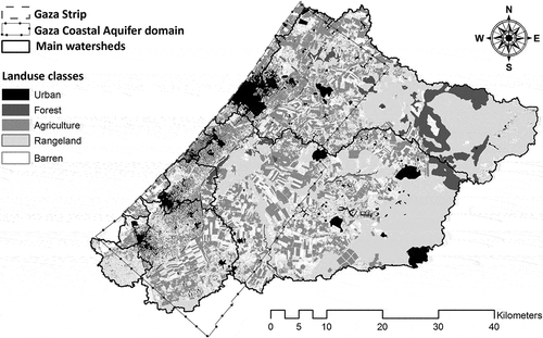
The land-use map (Fig. 5) was extracted through the processing of aerial images (resolution: 0.5 m) (MoP 2007) and historical data from Google Earth®. The supervised classification technique was used, based on ERDAS 9.3, to distinguish the main land-use classes in the study area. Manual digitization using ArcGIS 10.0 was performed to define the urban area and the layer was merged with the classified land-use image. Five main land-use classes were identified. The dominant categories are rangeland (50.2%), agricultural land (26.1%), barren land (13.8%) and forest land (5.3%). The urbanized areas represent 4.5% of the study area and 20% of the Gaza Strip.

Figure 5. Study area—land use.

3.2 SWAT model

The ArcSWAT model was used for the surface water modelling processes. ArcSWAT (ArcGIS extension) is a graphical user interface for the SWAT model (SWAT 2013). SWAT is a river basin or watershed-scale model developed to predict the impact of land management practices on water, sediment and agricultural chemical yields in large, complex watersheds with varying soils, land use and management conditions over long periods of time (Neitsch et al. 2011).

SWAT uses the water balance approach to simulate watershed hydrologic partitioning as described by Neitsch et al. (2011) in equation (1):

(1)

where SW_t is the final soil water content (mm), SW_o is the initial soil water content on day i (mm), t is the time (d), R_day is the amount of precipitation on day i (mm), Q_s is the amount of surface runoff on day i (mm), E_a is the amount of evapotranspiration on day i (mm), w_seep is the amount of water entering the vadose zone from the soil profile on day i (mm), and Q_gw is the amount of return flow on day i (mm).

The SWAT model provides two methods for estimating surface runoff volume, namely the Soil Conservation Service (SCS) curve number procedure (1972) and the Green and Ampt equation (1911). In the SCS method, the runoff for a given rainfall depth is calculated assuming a certain curve number (CN) for the surface related to the land use and the soil hydrologic group. The SCS method is based on an empirical formula that was developed from observations of several years of rainfall and runoff data obtained from a variety of combinations of soil, land use, topography and climate. SWAT defines percolation as the water that drains through the root zone into the aquifer. Downward flow occurs when the soil moisture exceeds the field capacity level of a soil layer. The downward flow rate is governed by the saturated hydraulic conductivity (K_s) of the soil layer. The lateral subsurface flow in the soil profile is calculated simultaneously with percolation. The lateral flow and surface runoff of all HRUs are summed for each sub-basin and then routed through the stream network (Quessar et al. 2009).

In this study, the SCS procedure was used to estimate the surface runoff. The Penman-Monteith equation was applied to estimate potential evapotranspiration. Manning’s equation was employed to define the rate and velocity of flow. Water was routed through the channel network using the variable storage routing method. A detailed description of different model components can be found in Neitsch et al. (2011).

3.3 Model running process

Under the umbrella of ArcSWAT, the spatial variability of soil, land use and land slope are accounted for by discretization of the watershed into sub-basins based on the topography and stream network. Each sub-basin consists of multiple HRUs representing characteristic combinations of soil, land-cover and land-slope properties. Figure 3 shows the discretization of the watersheds into 72 sub-basins, which contain 255 HRUs. In addition to the climatic data (Table A1), daily rainfall data from 19 stations were used to represent the rainfall distribution throughout the study area during the modelling period from 1 November 2004 to 31 October 2010 (Fig. 3). Daily minimum and maximum temperature data from five climate stations were used during the modelling period (Fig. 3) (Government portal–Israel 2013, PWA 2013). To satisfy the Penman-Monteith equation requirements (Neitsch et al. 2011) in the SWAT model, wind data taken from the climatic stations at heights of 10 m above ground were converted to 2 m above ground according to the equation (Potchter and Ben-Shalom 2013) .

3.4 Auto-calibration program

The SWAT-Calibration Uncertainty Procedure (SWAT-CUP) was used to perform calibration, validation and sensitivity analysis. SWAT-CUP contains the uncertainty analysis routine, namely Sequential Uncertainty Fitting version 2 (SUFI-2), which is a semi-automated inverse modelling procedure for a combined calibration–uncertainty analysis (Abbaspour et al. 2004). In SUFI-2, parameter uncertainty accounts for all sources of uncertainties such as uncertainty in driving variables (e.g. rainfall), conceptual model parameters, and measured data. It is possible to choose the uncertain parameters and the range of their physical values. The degree to which all uncertainties are accounted for is quantified as the percentage of measured data bracketed by the 95% prediction uncertainty (95PPU). The 95PPU is calculated at the 2.5% and 97.5% levels of the cumulative distribution of an output variable obtained through Latin hypercube sampling, disallowing 5% of the very bad simulations. In each running step in SWAT-CUP, previous parameter ranges are updated in such a way that the new ranges are always smaller than the previous ranges, and converge to the best simulation while considering a defined objective function (Abbaspour et al. 2004, Yang et al. 2008, Tang et al. 2012).

Considering the uncertainty analysis routine and a defined objective function in SWAT-CUP, model calibration and sensitivity analysis were performed. The flexibility of manual modification of the parameters, as well as the number of running steps between the auto-calibration runs, reflects the semi-automated approach of SWAT-CUP.

3.5 Model sensitivity analysis

Using SWAT-CUP, an initial sensitivity analysis was conducted to identify the most critical model parameters before starting the calibration process. The possible physical ranges of the parameter values were used in the initial sensitivity analysis to avoid excluding any sensitive parameter due to its nonlinear behaviour. Parameter sensitivities are determined by calculating the multiple regression system , which regresses parameters generated by the Latin hypercube against the objective function values (g), where b_i is the ith parameter, m is the total number of parameters, β_i is the partial slope coefficient, and α is the intercept (Abbaspour et al. 2007). The relative sensitivity values in SWAT-CUP are measured by t-tests and the corresponding p-values. The t-test provides a measure of sensitivity (larger absolute values are more sensitive), and p-value determines the significance of the sensitivity (lower p-value denotes more significance of the sensitivity measure).

3.6 Model calibration and validation

The simulated streamflow values were calibrated at the monthly time scale with the observed streamflow values for three discharge stations (WAI 2013) for the years 2004/05, 2007/08, and 2008/09 and validated at the monthly time scale for year 2009/10 (Fig. 3).

Generally, the main components of the calibration process include objective function(s) as a measure of goodness of fit between measured and simulated variables as well as optimization procedures. An auto-calibration process was performed using SWAT-CUP, which offers the possibility of selecting an objective function from the nine different available options. bR², which was used as the objective function, reflected the best match between simulated and observed flow, where b is the slope of the regression line between measured and simulated variables and R² is the coefficient of determination. The objective function is expressed as (Krause and Boyle 2005):

(2)

R² as well as b should be close to 1 in a high-performance model, and consequently the objective function (equation (2)) should be close to 1. A manual calibration was conducted to refine the auto-calibration, so that an appropriate balance was achieved regarding peak and low flows.

4 Model results and analysis

4.1 Sensitivity analysis, calibration and validation

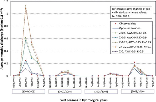
Table 2 shows the initial ranking of the sensitive parameters related to flow calibration based on 100 runs of the SWAT model. Spruill et al. (2000), White and Chaubey (2005), Niraula et al. (2012) and Wu and Liu (2013) agreed that these parameters were the most sensitive ones in their studies. The initial sensitivity analysis illustrates three sensitive packages (a package is a set of parameters), namely soil package, land-use and sub-basin parameters package, and groundwater package. The soil package was the most sensitive package, i.e. had the most sensitive parameters in the model. Understanding the interrelations between parameters within a package is worthwhile in order to obtain the optimum solution during the calibration process, especially if there is a high level of uncertainty. A manual sensitivity analysis was conducted to evaluate different relative changes of soil parameters at station 01 (Fig. 6). This analysis illustrates that soil parameters in the wet year 2004/05 have a higher sensitivity than in normal or dry years, which could be helpful in investigating the optimal model parameters.

Table 2. Initial estimation of sensitive parameters in SWAT model.

Parameter	Description	Type of change	Range of parameter values	t-stat	p-value	Rank
GWQMN	Threshold depth of water in the shallow aquifer required for return flow to occur (mm)	Replaced by value	0–5000^a	2.07	0.04	1
SOL_K	Saturated hydraulic conductivity (mm/h)	Relative change	−0.9–1^a	1.95	0.05	2
SOL_AWC	Available water capacity of the soil layer (mm H2O/mm soil)	Relative change	−0.5–0.5^b	−1.54	0.13	3
CN2	Initial SCS curve number for moisture condition II—pervious areas	Relative change	−0.3–0.2^b	1.04	0.3	4
REVAPMN	Threshold depth of water in the shallow aquifer for “revap” to occur (mm)	Replaced by value	0–500^a	−0.92	0.36	5
ALPHA_BF	Baseflow alpha factor (d)	Replaced by value	0–1^a	−0.78	0.44	6
ESCO	Soil evaporation compensation factor	Replaced by value	0–1^a	−0.49	0.63	7
SURLAG	Surface runoff lag coefficient	Replaced by value	0.05–24^a	0.48	0.63	8
GW_REVAP	Groundwater “revap” coefficient	Replaced by value	0.02–0.2^a	−0.31	0.76	9
SOL_Z	Depth from soil surface to bottom of layer mm	Relative change	−0.5–0.5^b	0.19	0.85	10
OV_N	Manning’s n value for overland flow	Replaced by value	0.01–3^a	−0.19	0.85	11
GW_DELAY	Groundwater delay time (d)	Replaced by value	0–500^a	0.07	0.95	12
CH_N2	Manning’s n value for the main channel	Replaced by value	0–0.3^a	0.04	0.97	13
CH_K2	Effective hydraulic conductivity in main channel (mm/h)	Replaced by value	0–25^a	0.04	0.97	14

^aDocumented in SWAT input data manual (SWAT 2013).

^bIdentified based on the authors’ experience in the study area.

Figure 6. Sensitivity analysis of varied relative changes in soil parameters.

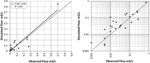
Tables 3 to 5 show the calibrated parameters for groundwater package, land-use and sub-basins package, and soil package. Calibration and validation statistics are summarized in Table 6. Considering all flows at the three stations through the calibration period, model efficiency measures for the monthly simulation R², bR² and E (Nash-Sutcliffe efficiency) are 0.87 (Fig. 7), 0.83 and 0.85, respectively, which indicate a very good fit between measured and simulated flows.

Table 3. Calibrated parameters—groundwater package.

Parameter	Description	Calibrated value
GWQMN	Threshold depth of water in the shallow aquifer required for return flow to occur (mm)	1000
REVAPMN	Threshold depth of water in the shallow aquifer for “revap” to occur (mm)	325
ALPHA_BF	Baseflow alpha factor (d)	0.6
GW_REVAP	Groundwater “revap” coefficient	0.025
GW_DELAY	Groundwater delay time (d)	160

Table 4. Calibrated parameters—land-use and sub-basins package.

Parameter	Description	Type of change
CN2	Initial SCS curve number for moisture condition II	No change for urban land use No change for rangeland except rangeland on brown rendzinas soil, CN2 increases by 6.5% For other land use, CN2 decreases by 5%
ESCO	Soil evaporation compensation factor	Replaced by 0.765
SURLAG	Surface runoff lag coefficient	Replaced by 9
OV_N	Manning’s n value for overland flow	No change (ranges from 0.1 to 0.15)

Table 5. Calibrated parameters—soil package.

Soil type	Layer	Calibrated value of soil parameters
		Sol_K (mm/h)	Sol_AWC (mm H2O/mm soil)	Sol_Z (mm)
Brown lithosols & loessial arid brown	1	1	0.305	70
	2	0.8	0.24	210
	3	0.4	0.18	350
Brown lithosols & loessial serozems	1	26	0.25	500
	2	2.3	0.25	1000
Brown rendzinas	1	0.6	0.29	870
Dark brown soils	1	4	0.2	650
Loess soils	1	12	0.1	1000
Loessial sandy	1	12	0.1	1000
Loessial serozems	1	13	0.32	750
	2	2.3	0.18	1500
Pararendzinas	1	210	0.1	250
	2	210	0.1	500
Regosols	1	12	0.1	1000
Sandy loess	1	4.3	0.2	1000
Sandy loess soil over loess	1	12	0.1	1000
Sandy regosols	1	210	0.07	750

Table 6. Summary of calibration and validation statistics.

Calibration results (monthly base)	Observed	Simulated
Average flows (m^3/s)	0.105	0.099
Standard deviation of flows (m^3/s)	0.21	0.19
Average of the highest 25% flows (m^3/s)	0.4	0.37
Average of the lowest 50% flows (m^3/s)	0.0041	0.0054
	Coefficient of determination, R^2	bR^2*	Nash-Sutcliffe efficiency, E
Station 01	0.95	0.89	0.95
Station 02	0.86	0.86	0.84
Station 03	0.89	0.85	0.86
All stations	0.87	0.83	0.85
Validation results (monthly base)
	Coefficient of determination, R^2	bR^2	Nash-Sutcliffe efficiency, E
Station 01	0.98	0.61	0.82
Station 02	0.95	0.90	0.94
Station 03	0.82	0.54	0.96
All stations	0.90	0.76	0.82

* b is the slope of the regression line between measured and simulated flow and it was modified according to equation (2).

Figure 7. Scatter plots between observed and simulated flow for three flow stations (in m³/s as average annual values).

Through the validation period, it was found that the model has good predictive capability with R², bR² and E values of 0.90, 0.76 and 0.82, respectively, for all flows at the three stations. Statistical model efficiency criteria (Table 6) attained the requirement of R² > 0.6 and E > 0.5, which is recommended by the SWAT developers (Santhi et al. 2001). As E values in calibration and validation periods are above 0.75, the performance rating of the model is very good (Moriasi et al. 2007).

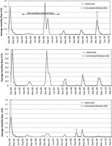
The monthly flow records contain mostly one or two flood events that can be considered as the real calibration level. Figure 8 shows that, through the calibration and the validation period, the observed and simulated flow at stations 01, 02 and 03 matched well. Few flow peaks are overestimated or underestimated by the model. The observed flow at station 03 in January 2005 is obviously higher than the simulated; an external flow from the reservoir upstream in a flood event through that month could be the main reason.

Figure 8. Comparison between observed and simulated flow at stations 01, 02 and 03.

A final sensitivity analysis was carried out to probe the real ranking of the sensitive parameters considering a range within ±10% change of the calibrated value. At 0.05 as the significant level, available water capacity of the soil layer (SOL_AWC), depth from soil surface to bottom of layer (SOL_Z), soil evaporation compensation factor (ESCO), and initial SCS curve number for moisture condition II (CN2) have the highest t-test values and are thus the most sensitive parameters (Table 7). Table 8 shows the average values of the most sensitive parameters considering the land-use classes with the study area.

Table 7. Final sensitivity analysis of sensitive parameters.

Parameter	Description	t-stat	p-value	Final rank
SOL_AWC	Available water capacity of the soil layer (mm H2O/mm soil)	6.0	0.00	1
SOL_Z	Depth from soil surface to bottom of layer mm	4.6	0.00	2
ESCO	Soil evaporation compensation factor	−2.8	0.01	3
CN2	Initial SCS curve number for moisture condition II	−2.3	0.03	4
OV_N	Manning’s n value for overland flow	1.4	0.17
GW_DELAY	Groundwater delay time (d)	−1.4	0.17
SURLAG	Surface runoff lag coefficient	1.1	0.31
SOL_K	Saturated hydraulic conductivity (mm/h)	−1.0	0.35
GW_REVAP	Groundwater “revap” coefficient	−0.8	0.43
GWQMN	Threshold depth of water in the shallow aquifer required for return flow to occur (mm)	−0.7	0.47
REVAPMN	Threshold depth of water in the shallow aquifer for “revap” to occur (mm)	0.5	0.62
ALPHA_BF	Baseflow alpha factor (d)	0.0	0.98

Table 8. Average values of the most sensitive model parameters, as calculated by SWAT for land-use classes within the study area. CN: curve number; AWC: available water capacity of the soil layer.

Average within:	Most sensitive model parameters^a
	Land-use parameters: CN	Soil parameters^b: AWC (mm H2O/total soil depth)^c
Agricultural land	68.0	122.1
Barren land	79.1	115.1
Rangeland	53.3	144.4
Forest land	53.1	126.1
Urban land (pervious and impervious)	80.5	102.8
Overall study area	61.4	132.0
Gaza Strip boundary	67.2	98.4

^aESCO, a highly sensitive parameter (Table 7), has a constant value among the HRUs (0.765).

^bEven though the sensitivity analysis illustrates that the saturated hydraulic conductivity (K_s) of soil is not a highly sensitive parameter, it may be valuable in understanding the watershed conditions. Within the study area, the average calibrated K_s was 18 mm/h and ranged between 0.6 and 210 mm/h (see Table 5).

^cAWC is a function of (SOL_AWC and SOL_Z).

4.2 Water budget components

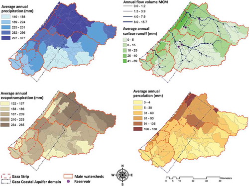
Spatial variability was investigated in the study area by connecting the model output files and the watershed themes in the ArcGIS environment. Figure 9 shows the spatial distribution of the rainfall and the water budget components throughout the study area. The average annual rainfall decreases gradually from north to south as well as from west to east. The average annual surface runoff varies from 0 mm in the southeast to 89 mm in the northwest. The maximum average annual percolation (124 mm) is in the northern part of the study area. The average annual actual evapotranspiration varies between sub-basins within a broad range (132–265 mm). Figure 9 displays the differences between the northern and southern watersheds in surface water yield, as well as the effects of reservoirs on the natural extents of the watersheds. The maximum average annual flow-volume was 15.7 hm³ in the largest northern watershed. Simulated percolation, surface runoff and evapotranspiration represent on average 22.4%, 11.7% and 65.0%, respectively, of the rainfall quantities within the Gaza Strip boundary, whereas these values are 17.9%, 6.5% and 74.5%, respectively, considering the aquifer domain boundary. Table 9 shows the average annual values of the water balance components and their ranges among sub-basins.

Table 9. Average annual values of water balance components and their ranges among sub-basins (2004–2010).

Water balance components	Within the study area		Within the Gaza Strip boundary
	Average (mm)	Range among sub-basins (mm)	Average (mm)	Range among sub-basins (mm)
Precipitation	258.4	139.9–377.2	277.4	216.8–340.0
Surface runoff	12.6	0.0–89.2	32.5	0.2–89.2
Lateral flow	4.3	0.01–37.2	2.3	0.03–6.2
Baseflow*	~0.0	0.0–0.3	0.0	0.0
Percolation	38.6	0.0–124.5	62.2	24.3–117.2
Evapotranspiration	201.7	132.4–265.1	180.4	146.2–227.8
Potential evapotranspiration	1517.4	1368.8–1712.4	1414.2	1368.8–1520.8
Change in soil water storage	1.2	0.0–17.8	0.8	0.0–12.7

*Although there are some small springs in specific sub-basins, they are not sufficient to generate significant baseflow.

Figure 9. Average annual rainfall distribution and water budget components (2004–2010).

4.3 Urban area analysis

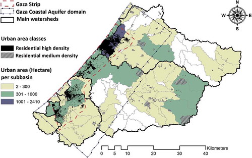
Urbanization is a major driver of additional pressures (both qualitative and quantitative) on the environment (Rozos and Makropoulos 2012). Traditionally, the response of watersheds to urban development has been measured in terms of changes in the flow regime and groundwater recharge. There are two patterns of urbanization within the study area, namely Gaza Strip cities and Israel colonies. Great concerns have emerged in recent years about uncontrolled urban expansion in the Gaza Strip (Isaac et al. 2006). Urban development and infrastructure encroach upon agricultural land and rangelands creating additional pressure on the limited water resources of the Gaza Strip. The Gaza Strip cities have a high residential density (impervious area represents about 60% of the total urban area). The Israeli colonies or cities in the study area have low to moderate residential density (impervious area represents 12–38% of the total urban area) and are located outside the Gaza Strip. There were scattered Israeli colonies in the Gaza Strip, but the Israeli government evacuated them in 2005 (Isaac et al. 2006). Figure 10 shows the variety of the urban areas in terms of high or medium residential density at sub-basin level. The hydrologic response to the urban area change was simulated in this study. The impacts of 10, 20, 30 and 50% increases in the residential high density area (urban area in the Gaza Strip) on the percolation and the surface runoff were investigated. The agricultural land and rangeland decreased equally with the continuous increase in urban areas. Unique linear relationships between the relative change in urban area and the corresponding relative change in surface water and percolation were concluded for different sub-basins. The equation y = αx is the general formula to simulate the surface runoff or percolation response (y) to the urban change (x). Each sub-basin has a unique linear relation slope (α), which represents a sensitivity factor of the hydrological components.

Figure 10. Urban area distribution.

Figure 11 presents different linear relations for the sub-basins having the highest built-up area. Spatial evaluation of the surface runoff and the percolation response to the urban expansion were carried out considering the linear relation slope (α) as urban-surface runoff index (USI) or urban-percolation index (UPI). The USI reflects the percentage change in surface runoff due to a 1% increase in urban area at sub-basin level. Similarly, the UPI reflects the percentage change in percolation due to a 1% increase in urban area at sub-basin level. Figure 12 shows the spatial distribution of the USI from 0 to around 1 and exhibits the UPI values (from 0 to −0.41) on the basis of sub-basins.

Figure 11. Linear relationship between urban area change and percolation/surface runoff.

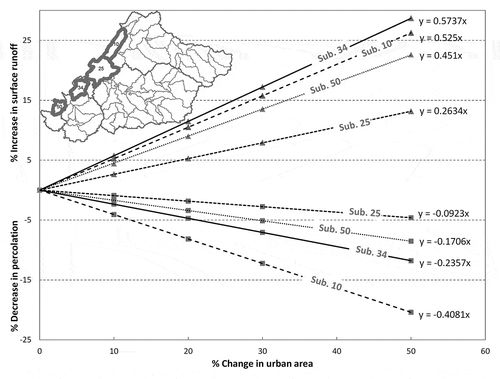
Figure 12. Urban-surface runoff index and urban-percolation index.

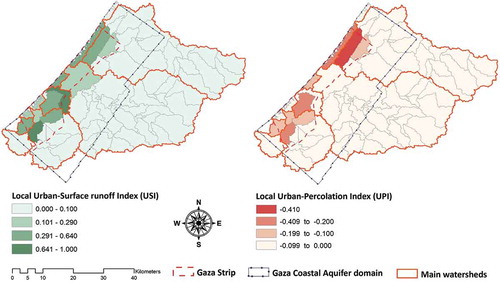
The USI and the UPI give an indication for each sub-basin about the reaction of the hydrological system to the urban area change. However, the indexes do not reflect the relative impact between sub-basins on the aquifer percolation or on the overall surface runoff. In addition to the hydrological components, variation of the sub-basin geometry has an obvious impact on USI and UPI.

The influence on total aquifer percolation and overall surface runoff within the aquifer domain due to urban area change was quantified in a spatial approach. The global urban-surface runoff index (GUSI) and global urban-percolation index (GUPI) were derived:

(3)

(4)

where n is the total number of sub-basins shared in the aquifer domain, i is the sub-basin number (from 1 to n), A_i is the area of sub-basin i, S_i is the surface runoff of sub-basin i, and P_i is the percolation of sub-basin i.

Figure 13 depicts the spatial variability of the percentage change in overall surface runoff across the aquifer domain due to urban area expansion by 1% at sub-basin level (GUSI). Similarly, it depicts the spatial variability of the percentage change in aquifer recharge due to urban area expansion by 1% at sub-basin level (GUPI). A larger urban area in a sub-basin gives a higher GUSI and a higher negative GUPI. The large and high density urban area in the northern Gaza Strip is translated into a high GUSI and a high negative GUPI. The previous indexes are valid as long as there is no significant change in the hydrological characteristics of the surrounding areas due to the urban area expansion.

Figure 13. Global urban-surface runoff index and global urban-percolation index.

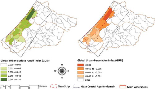
The Coastal Municipalities Water Utility (CMWU 2010) reported that the Gaza coastal aquifer has two sensitive areas of groundwater depression, i.e. in the north where the groundwater level drops more than 4 m below the mean sea level and in the south where it drops more than 12 m. In this case, the UPI can support the decision maker in the evaluation of different urban change scenarios in the sub-basins in the north and south of the Gaza Strip. On the other hand, the GUPI and the GUSI can contribute to the development of spatial sustainability indicators for the Gaza coastal aquifer.

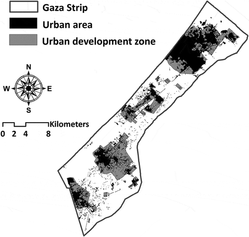
The regional plan for the Gaza Strip (2020) considered the natural resources areas in the planning process of the urban development zone (MoP 2007). Figure 14 shows that the southern urban development zone is directed to the east (lower groundwater quality) and not to the west (higher groundwater quality). By intersecting Figs 13 and 14, the northern urban development zone has the highest negative GUPI (Fig. 13). The urban development zone with high population density will increase the GUSI with increasing negative GUPI, representing a threat to the aquifer sustainability. Decreasing the impervious area in the urban development zone in the north of the Gaza Strip as far as possible is a substantial approach towards a solution. Decreasing the built-up area by introducing taller buildings in the development zone relative to the existing urban area is recommended. Water-saving schemes such as rainwater harvesting and greywater treatment can significantly reduce the pressures of new urban development (Rozos and Makropoulos 2012). Surface runoff harvesting systems are therefore recommended for the urban development zone, especially in the northern area of the Gaza Strip.

Figure 14. Urban development zone (2020) for the Gaza Strip.

5 Summary and conclusions

This study quantifies the impact of urban area expansion on the coastal aquifer recharge and surface runoff of the semi-arid watersheds intersecting with the Gaza Strip. The results show that the SWAT model could simulate water budget components adequately within these complex watersheds. Based on a semi-automated approach of calibration and sensitivity analysis using SWAT-CUP software, the most sensitive parameters are available water capacity of the soil layer, depth from soil surface to bottom of layer, soil evaporation compensation factor, and initial SCS curve number for moisture condition II. Therefore, as the soil package of the SWAT parameters has the most sensitive parameters, this package is can be defined as the most sensitive.

The simulations reveal a considerable spatial variability of the water budget components throughout the study area. The simulated percolation, surface runoff and evapotranspiration represent on average 22.4%, 11.7% and 65.0%, respectively, of the rainfall quantities within the Gaza Strip boundary, whereas these values are 17.9%, 6.5% and 74.5%, respectively, considering the aquifer domain boundary. The average annual surface runoff varies from 0 mm in the southeast to 89 mm in the northwest. The maximum average annual percolation (124 mm) takes place in the northern part of the study area. The average annual evapotranspiration ranges widely from 132 to 265 mm. The maximum average annual flow-volume was 15.7 hm³ in the largest northern watershed, whereas it decreased sharply in the southern main watersheds to around 4 hm³. Based on SWAT, the relationship between the relative change in urban area and the corresponding relative change in surface runoff or percolation can be estimated to be nearly linear. The urban-surface runoff index (USI), which reflects the percentage change in surface runoff due to a 1% increase in urban area at sub-basin level, ranges from 0 to around 1, while the urban-percolation index (UPI), which represents the percentage change in percolation due to a 1% increase, ranges from 0 to −0.41. To identify the relative impact between sub-basins, the global urban-surface runoff index (GUSI) and global urban-percolation index (GUPI) were derived to quantify the influence on the total aquifer percolation and the overall surface runoff due to (high density) urban area change. The USI and UPI can support decision makers in the micro-level evaluation of different urban change scenarios in the sub-basins. For instance, the UPI can be used to evaluate the influence of urban area change on the sensitive areas of groundwater depression related to specific sub-basins. Whereas GUSI and GUPI are macro-level factors, they can be of significant importance for framing sustainable planning for the water resources in the Gaza Strip. Based on GUPI and GUSI, decreasing the impervious areas and developing surface runoff harvesting systems in the urban development zone of the Gaza Strip are important options for aquifer sustainability, especially in the northern area.

Acknowledgements

The first author thanks the German Academic exchange service (DAAD) for the PhD scholarship. We thank the Fiat Panis Foundation for supporting this research during the period of data collection.

Disclosure Statement

No potential conflict of interest was reported by the authors.

Appendix A

Table A1 shows the climatic data used in the modelling process.

Table A1. Monthly climatic data for study area.

Beersheva (Meteorological Service database 2013)
Month	Jan	Feb	Mar	Apr	May	Jun	Jul	Aug	Sep	Oct	Nov	Dec
Tmax (°C)	17.9	19.2	23.3	27.3	30.2	33.5	34.8	35.4	33.3	29.6	24.7	20.1
Tmin (°C)	7.0	8.3	10.3	13.2	15.8	19.3	21.4	21.9	20.4	16.8	12.0	8.4
Mean rainfall (mm/month)	29.8	43.2	16.0	12.1	1.0	0.0	0.0	0.0	0.8	10.9	21.7	28.0
Dew point (°C)	4.0	6.0	6.8	7.9	11.4	15.3	17.7	19.1	17.3	14.3	8.8	5.1
Mean relative humidity (%)	64.7	66.9	60.8	54.4	56.3	58.3	60.6	63.1	62.5	63.7	60.8	62.4
Wind speed (m/s) (10 m height)	2.4	2.5	2.5	2.7	2.6	2.6	2.4	2.3	2.4	2.2	2.1	2.2
Pan evaporation (mm/d)*	2	2.6	3.8	5.9	7.6	8.6	8.4	7.8	6.6	5	3.4	2.1
Global solar radiation (MJ/m^2 per day)	10.7	13.6	18.1	22.8	26.3	28.9	27.9	25.6	22.0	16.8	12.5	10.1

* Average value, 1988–2000.

Table

Lahav (Meteorological Service database 2013)
Month	Jan	Feb	Mar	Apr	May	Jun	Jul	Aug	Sep	Oct	Nov	Dec
Tmax (°C)	15.8	17.0	20.8	25.2	28.5	31.8	33.1	33.6	31.4	27.5	22.5	18.0
Tmin (°C)	7.4	8.2	10.0	12.6	14.5	17.7	19.6	20.4	19.4	16.7	13.2	9.4
Mean rainfall (mm/month)	53.7	54.1	28.8	11.7	0.6	0.0	0.0	0.0	0.0	5.8	64.7	54.4
Dew point (°C)	2.9	5.0	6.0	7.4	10.4	14.3	17.3	18.2	16.5	13.5	8.3	4.4
Mean relative humidity (%)	60.9	64.2	59.4	53.9	52.4	54.8	59.0	60.2	62.0	62.2	57.8	59.5
Wind speed (m/s) (10 m height)*	2.3	2.6	2.8	2.5	2.6	2.8	2.9	2.6	2.3	1.9	4.9	2.8
Global solar radiation (MJ/m^2 per day)**	10.0	12.9	17.5	21.9	25.5	28.0	27.1	24.8	21.3	16.0	11.8	8.92

* Wind speed data for Hebron (Ismail et al. 2013).

** Calculated based on the interpolation between Negba station and Beersheva station.

Table

Ein-Habsor (Meteorological Service database 2013)
Month	Jan	Feb	Mar	Apr	May	Jun	Jul	Aug	Sep	Oct	Nov	Dec
Tmax (°C)	18.0	19.2	22.7	26.1	27.9	30.9	32.2	32.5	31.1	28.0	24.2	20.1
Tmin (°C)	7.6	8.6	10.3	12.6	15.1	18.5	20.7	21.5	20.2	17.2	12.8	9.3
Mean rainfall (mm/month)	40.1	51.7	21.2	10.6	0.4	0.0	0.0	0.0	0.0	31.3	42.1	62.6
Dew point (°C)	5.9	7.6	8.5	10.6	13.8	17.5	19.8	20.8	18.7	15.8	11.3	7.3
Mean relative humidity (%)	70.3	73.3	68.8	66.7	68.4	69.6	70.9	72.6	68.9	71.0	69.7	69.0
Wind speed (m/s) (10 m height)	2.7	2.8	2.7	2.8	2.5	2.4	2.3	2.1	2.2	2.2	2.2	2.4
Pan evaporation (mm/d)*	2.4	2.9	4.1	6.1	7.1	7.8	7.7	7.1	6.2	4.8	3.5	2.5
Global solar radiation (MJ/m^2 per day)	9.6	12.8	16.9	21.2	25.6	27.6	26.7	24.0	21.0	15.5	11.6	9.0

* Average value, 1988–2000.

Table

Negba (Meteorological Service database 2013)
Month	Jan	Feb	Mar	Apr	May	Jun	Jul	Aug	Sep	Oct	Nov	Dec
Tmax (°C)	17.5	18.3	21.4	25.2	27.2	30.0	31.5	31.9	30.8	27.6	23.9	19.6
Tmin (°C)	7.8	8.5	10.0	12.4	14.9	18.7	21.2	22.1	21.0	17.9	13.2	9.5
Mean rainfall (mm/month)	99.9	71.9	33.3	12.9	3.1	0.0	0.0	0.0	0.0	53.4	47.0	71.9
Dew point (°C)	6.1	8.0	9.1	10.7	13.9	17.7	20.1	20.9	18.5	15.6	10.6	7.2
Mean relative humidity (%)	70.3	75.0	70.9	66.8	68.2	69.7	71.1	71.6	66.5	67.4	64.9	67.7
Wind speed (m/s) (10 m height)	2.9	3.1	3.0	3.1	2.9	2.9	2.9	2.8	2.8	2.7	2.6	2.6
Pan evaporation (mm/d)*	1.9	2.5	3.4	5.2	6.3	7.2	7.3	6.8	6.1	4.6	3.1	2.1
Global solar radiation (MJ/m^2 per day)	9.4	12.2	16.8	21.1	24.8	27.2	26.3	24.0	20.5	15.3	11.2	8.9

* Average value, 1988–2000.

Table

Gaza
Month	Jan	Feb	Mar	Apr	May	Jun	Jul	Aug	Sep	Oct	Nov	Dec
Tmax (°C)^a	18.0	18.4	19.6	24.7	24.8	27.1	29.8	31.9	30.0	27.6	24.2	20.8
Tmin (°C)^a	10.3	11.4	11.9	15.8	18.6	21.6	23.2	25.0	22.7	20.4	17.4	12.7
Mean rainfall (mm/month)^b	75.9	71.7	27.7	5.5	0.2	0.0	0.0	0.0	0.0	26.2	55.8	52.0
Dew point (°C)^c	8.0	9.0	9.0	14.0	17.0	20.0	22.0	23.0	20.0	17.0	16.0	10.0
Mean relative humidity (%)^a	66.0	69.0	64.0	67.0	73.0	77.0	76.0	75.0	65.0	66.0	72.0	62.0
Wind speed (m/s) (10 m height)^d	2.7	2.8	2.72	2.8	2.52	2.4	2.3	2.1	2.2	2.2	2.24	2.4
Pan evaporation (mm/d)^e	2.5	2.9	3.7	4.6	5.4	6.0	6.3	6.1	5.6	4.2	3.3	2.6
Global solar radiation, (MJ/m^2 per day)^f	9.5	12.5	16.9	21.2	25.2	27.4	26.5	24.0	20.8	15.4	11.4	9.0

^aGhabayen (2001), average values for 20 years.

^bPWA (2013) archived data (from 2004 to 2010).

^cCalculated based on the relation between mean temperature and relative humidity.

^dEin-Habsor station.

^eMinistry of Agriculture (MoA 2013)-Gaza (average monthly value, 1996–2006).

^fCalculated based the interpolation between Negba station and Ein-Habsor station.

References

- Abbaspour, K.C., Johnson, C.A., and Genuchten, T., 2004. Estimating uncertain flow and transport parameters using a sequential uncertainty fitting procedure. Vadose Zone Journal, 1352, 1340–1352. doi:10.2113/3.4.1340.
- Abbaspour, K.C., et al., 2007. Modelling hydrology and water quality in the pre-alpine/alpine Thur watershed using SWAT. Journal of Hydrology, 333 (2–4), 413–430. doi:10.1016/j.jhydrol.2006.09.014.
- Aish, A., Batelaan, O., and De Smedt, F., 2010. Distributed recharge estimation for groundwater modelling using WETSPASS, case study: Gaza Strip, Palestine. The Arabian Journal for Science and Engineering, 35 (1B), 155–164.
- Ajjur, S. and Mogheir, Y., 2012. Effect of climate change on the groundwater resources (Gaza Strip case study). International Journal of Sustainable Energy and Environment, 1 (8), 136–149.
- Baaloush, H., 2008. Analysis of nitrate occurrence and distribution in groundwater in the Gaza Strip using major ion chemistry. Global NEST Journal, 10 (3), 337–349.
- Chu, J., Zhang, C., and Zhou, H., 2010. Study on interface and frame structure of SWAT and MODFLOW models coupling. Geophysical Research–EGU General Assembly Conference Abstracts, 12, 4559.
- Coastal Municipalities Water Utility (CMWU)–Gaza, 2010. Water Status in the Gaza Strip and Future Plans, Annual report [Online], Available from: http://www.cmwu.ps [Accessed August 2013].
- Dan, J., et al., 1976. The soil of Israel (Historical Palestine) with map 1:500,000. Bet Dagan: Ministry of Agriculture, Division of Scientific Publications.
- Dong, W., et al., 2013. Relative effects of human activities and climate change on the river runoff in an arid basin in northwest China. Hydrological Processes, published online. doi:10.1002/hyp.9982.
- Dudeen, B., 2001. The soils of Palestine (The West Bank and Gaza Strip) current status and future perspectives. Options Méditerranéennes: Série B. Etudes et Recherches, 34, 203–225.
- Fadil, A., et al., 2011. Hydrologic modelling of the Bouregreg watershed (Morocco) using GIS and SWAT Model. Journal of Geographic Information System, 3 (4), 279–289. doi:10.4236/jgis.2011.34024.
- Food and Agriculture Organization of the United Nations FAO, 2006. Guidelines for soil description. Rome: FAO. ISBN 92-5-105521-1.
- Geron, R., Amit, R., and Grossman, S., 1985. Dust availability in desert terrains, a study in the deserts of Israel and the Sinai. Institute of Earth Sciences-the Hebrew University of Jerusalem, project for the US Army Research, and Development and Standardization Group-UK. Contract No. DAJA45-83-C-0041.
- Ghabayen, S., 2001. Archived data about Gaza Strip, Utah State University [Online]. Available from: http://hydrology.neng.usu.edu/giswr/archive00/termpa-pers/ghabayen.htm [Accessed May 2010]
- Government portal–Israel, 2013. Metrological data [Online]. Available from: http://data.gov.il/ims [Accessed August 2013].
- Hamad, J., et al., 2012. Modeling the impact of land-use change on water budget of Gaza Strip. Journal of Water Resource and Protection, 4, 325–333. doi:10.4236/jwarp.2012.46036.
- Hamdan, S., Troeger, S., and Nassar, A., 2007. Stormwater availability in the Gaza Strip, Palestine. International Journal of Environment and Health, 1 (4), 580–594. doi:10.1504/IJENVH.2007.018582.
- HWE (House of Water and Environment), 2010. Ground Water Protection Plan for Gaza Coastal Aquifer project, Final report [Online]. Available from: http://www.hwe.org.ps/ [Accessed March 2011].
- Isaac, J., et al., 2006. Analysis of urban trends and landuse changes in the Gaza Strip. Applied Research Institute–Jerusalem (ARIJ) [Online]. the report Available from: http://www.arij.org/publications/books-a-atlases/ [Accessed August 2013].
- Ismail, M., Moghavvemi, M., and Mahlia, T., 2013. Energy trends in Palestinian territories of West Bank and Gaza Strip: Possibilities for reducing the reliance on external energy sources. Renewable and Sustainable Energy Reviews, 28, 117–129. doi:10.1016/j.rser.2013.07.047.
- Karcher, S., VanBriesen, J., and Nietch, C., 2013. Alternative land-use method for spatially informed watershed management decision making using SWAT. Journal of Environmental Engineering, 139 (12), 1413–1423. doi:10.1061/(ASCE)EE.1943-7870.0000770.
- Khalaf, A., Al-Najar, H., and Hamed, J., 2006. Assessment of rainwater run-off due to the proposed regional plan for Gaza governorates. Journal of Applied Sciences, 6 (13), 2693–2704. doi:10.3923/jas.2006.2693.2704.
- Kim, Y., Band, L., and Song, C., 2013. The influence of forest regrowth on the stream discharge in the north Carolina piedmont watersheds. JAWRA Journal of the American Water Resources Association, published online. doi:10.1111/jawr.12115.
- Krause, P. and Boyle, D.P., 2005. Advances in geosciences comparison of different efficiency criteria for hydrological model assessment. Advances in Geosciences, 5, 89–97. doi:10.5194/adgeo-5-89-2005.
- Laronne, J.B., Alexandrov, Y., and Reid, I., 2004. Surface water characterization and utilization in the middle east, respectively exemplified by Nahal Eshtemoa (Wadi Samoa) & the Shiqma Besor (Wadi Gaza) reservoirs, Israel. In: H. Shuval and H. Dwiek, eds. Water for life in the Middle East, Vol. 2. Jerusalem: Israel/Palestine center for research and information, 680–692.
- Levick, L., et al., 2004. Adding global soils data to the Automated Geospatial Watershed Assessment Tool (AGWA). The 2nd International Symposium on Transboundary Waters Management, Tucson - Arizona [Online]. Available from: http://www.tucson.ars.ag.gov/agwa/docs/pubs/sahra-global_soils.pdf [Accessed August 2013].
- McCuen, R., 2004. Hydrology analysis and design. 4th ed. Upper Saddle River, NJ: Prentice Hall.
- Memarian, H., et al., 2014. SWAT-based hydrological modelling of tropical land use scenarios. Hydrological Sciences Journal, Published online: 10 Feb 2014. doi:10.1080/02626667.2014.892598.
- Meteorological Service database, 2013. Archived data [Online]. Available from http://www.ims.gov.il/ims [Accessed August 2013].
- MoA (Ministry of Agriculture), 2013. Archived data. Gaza–Palestine: (MoA).
- MoP (Ministry of Planning), 2007. Archived data. Gaza–Palestine: (MoP).
- Moriasi, D.N., et al., 2007. Model evaluation guidelines for systematic quantification of accuracy in watershed simulations. T.ASABE, 50 (3), 885–900. doi:10.13031/2013.23153.
- Neitsch, S., et al., 2011. The soil and water assessment tool theoretical documentation version 2009, technical report. Texas water resources institute, No. 406 [Online]. Available from: http://twri.tamu.edu/reports/2011/tr406.pdf [Accessed August 2013].
- Niraula, R., et al., 2012. Multi-gauge calibration for modelling the semi-arid Santa Cruz watershed in Arizona-Mexico border area using SWAT. Air, Soil and Water Research, 5, 41–57. doi:10.4137/ASWR.S9410.
- NRCCA (Northeast Region Certified Crop Adviser), Cornell University–New York–US, 2013. Soil hydrology [Online]. Available from: http://nrcca.cals.cornell.edu/soil/CA2/CA0212.1-3.php [Accessed August 2013].
- PCBS (Palestinian Central Bureau of Statistics), 2006. Palestinians at the end of year 2006, Ramallah–Palestine [Online]. Available from: http://www.pcbs.gov.ps [Accessed August 2013].
- Potchter, O. and Ben-Shalom, H., 2013. Urban warming and global warming: combined effect on thermal discomfort in the desert city of Beer Sheva, Israel. Journal of Arid Environments, 98, 113–122. doi:10.1016/j.jaridenv.2013.08.006.
- PWA (Palestinian Water Authority), 2013. Archived data. Gaza–Palestine: PWA.
- Quessar, M., et al., 2009. Modeling water-harvesting systems in the arid south of Tunisia using SWAT. Hydrology and Earth System Sciences, 13, 2003–2021. doi:10.5194/hess-13-2003-2009.
- Rahman, M., et al., 2013. An integrated study of spatial multicriteria analysis and mathematical modelling for managed aquifer recharge site suitability mapping and site ranking at Northern Gaza coastal aquifer. Journal of Environmental Management, 124, 25–39. doi:10.1016/j.jenvman.2013.03.023.
- Rozos, E. and Makropoulos, C., 2012. Assessing the combined benefits of water recycling technologies by modelling the total urban water cycle. Urban Water Journal, 9 (1), 1–10. doi:10.1080/1573062X.2011.630096.
- Santhi, C., et al., 2001. Validation of the SWAT model on a large river basin with point and nonpoint sources. Journal of the American Water Resources Association, 37 (5), 1169–1188. doi:10.1111/j.1752-1688.2001.tb03630.x.
- Shadeed, S. and Almasri, M., 2010. Application of GIS-based SCS-CN method in West Bank catchments, Palestine. Water Science and Engineering, 3 (1), 1–13.
- Singh, A., et al., 2014. Assessing the performance and uncertainty analysis of the SWAT and RBNN models for simulation of sediment yield in the Nagwa watershed, India. Hydrological Sciences Journal, 59 (2), 351–364. doi:10.1080/02626667.2013.872787.
- Spruill, C., Workman, R., and Taraba, J., 2000. Simulation of daily and monthly stream discharge from small watersheds using SWAT model. American Society of Agricultural Engineers, 43 (6), 1431–1439. doi:10.13031/2013.3041.
- SWAT (Soil and Water Assessment Tool), 2013. Model website [Online]. Available from: http://swat.tamu.edu/ [Accessed August 2013].
- Tang, F.F., Xu, H.S., and Xu, Z.X., 2012. Model calibration and uncertainty analysis for runoff in the Chao River Basin using sequential uncertainty fitting. Procedia Environmental Sciences, 13, 1760–1770. doi:10.1016/j.proenv.2012.01.170.
- USGS (US Geological Survey), 2012 EarthExplorer [Online]. Available from: http://earthexplorer.usgs.gov [Accessed March 2012].
- Valdivieso, F. and Sendra, J., 2013. Semi-distributed hydrological model with scarce information: an application to a large south-American binational basin. Journal of Hydrologic Engineering, published online. doi:10.1061/(ASCE)HE.1943-5584.0000853.
- Wang, R., et al., 2013. Individual and combined effects of land use/cover and climate change on Wolf Bay watershed streamflow in southern Alabama. Hydrological Processes, published online. doi:10.1002/hyp.10057.
- Water Authorities, Israel (WAI). 2013. Hydrological annual reports. [Online] [Accessed August 2013]. Available from http://www.water.gov.il/hebrew/Pages/home.aspx
- White, K. and Chaubey, I., 2005. Sensitivity analysis, calibration and validations for a multisite and multivariable SWAT model. Journal of the American Water Resources Association, 41 (5), 1077–1089. doi:10.1111/j.1752-1688.2005.tb03786.x.
- Wu, Y. and Liu, S., 2013. Improvement of the R-SWAT-FME framework to support multiple variables and multi-objective functions. Science of the Total Environment, 466/467, 455–466. doi:10.1016/j.scitotenv.2013.07.048.
- Yang, J., et al., 2008. Comparing uncertainty analysis techniques for a SWAT application to the Chaohe Basin in China. Journal of Hydrology, 358 (1–2), 1–23. doi:10.1016/j.jhydrol.2008.05.012.
- Zhang, Y., 2005. Development of study on model-SWAT and its application. Progress in Geography, 24 (5), 121–130.