Point process models for fine-resolution rainfall

Abstract

In a recent development in the literature, a new temporal rainfall model, based on the Bartlett-Lewis clustering mechanism and intended for sub-hourly application, was introduced. That model replaced the rectangular rain cells of the original model with finite Poisson processes of instantaneous pulses, allowing greater variability in rainfall intensity over short intervals. In the present paper, the basic instantaneous pulse model is first extended to allow for randomly varying storm types. A systematic comparison of a number of key model variants, fitted to 5-min rainfall data from Germany, then generates further new insights into the models, leading to the development of an additional model extension, which introduces dependence between rainfall intensity and duration in a simple way. The new model retains the original rectangular cells, previously assumed inappropriate for fine-scale data, obviating the need for the computationally more intensive instantaneous pulse model.

Editor D. Koutsoyiannis

Résumé

Un nouveau modèle temporel de la pluie a récemment été proposé dans la littérature, basé sur un processus de Bartlett-Lewis et destiné à des applications à des échelles de temps inférieures à l’heure. Ce modèle remplace les cellules rectangulaires du modèle original par des processus de Poisson finis d’impulsions instantanées, qui permettent une plus grande variabilité de l’intensité de la pluie sur de courts intervalles. Dans le présent article, le modèle d’impulsions instantanées a d’abord été généralisé pour permettre d’obtenir différents types d’averses. Une comparaison systématique de plusieurs variantes importantes du modèle, calées sur des données temporelles au pas de temps de 5 minutes provenant d’Allemagne, a ouvert de nouvelles perspectives sur ces modèles, menant au développement d’une nouvelle extension du modèle introduisant de façon simple une dépendance entre l’intensité de la pluie et sa durée. Le nouveau modèle conserve les cellules rectangulaires d’origine, qui avaient été jugées inadéquates pour des données à échelles fines, évitant ainsi le recours au modèle d’impulsions instantanées pour lequel les calculs sont plus complexes.

Key words:

• rainfall
• stochastic models
• Bartlett-Lewis models
• Poisson cluster processes
• sub-hourly
• fine-scale

Mots clefs:

• pluie
• modèle stochastique
• modèle de Bartlett-Lewis
• processus de Poisson
• infra-horaire
• échelle fine

1 INTRODUCTION

For both operational and design purposes, hydrologists require long series of rainfall. The time-steps required vary from the daily (for large catchment studies) down to a few minutes for small, typically urban catchments. Observed data series are, however, often too short, particularly at fine time-scales. While there is an abundance of long daily records in the UK, the number of hourly rainfall records longer than 10 years is of the order of 100. Records of 5- or 10-min rainfalls are generally short, as they are recorded over the duration of a particular study (e.g. Hyrex experiment, Moore and Hall 2000), and thus include only a limited range of rainfall variability.

The possibility of obtaining ensembles of long series of realistic rainfall data at a range of scales has been the motivation for the development of stochastic rainfall generators over the past four decades. The realism of the data is typically measured by the model’s ability to reproduce standard statistics of the time series of rainfall depth (mean, variance, skewness, autocorrelations), the proportion of dry periods, and the extreme behaviour of rainfall depths at different scales of interest. Unsurprisingly, given the complexity and diversity of the precipitation generating mechanisms, the accurate reproduction of so many features has so far eluded existing rainfall models. Clear progress is, however, detectable, and this paper is a contribution to one well-established approach to rainfall modelling.

This approach involves the representation of the physical rainfall process in a realistic, if simplified way, such that the hierarchical structure of rainfall is explicitly incorporated and the parameters have interpretable meanings. Introduced in two seminal papers by Rodriguez-Iturbe et al. (1987, 1988), it applies Poisson cluster processes to the underlying unobserved continuous-time rainfall process, with the rainfall contributed by a sequence of cells within storms; in these models, discrete-time properties are obtained by aggregation and used to fit to discrete observations. One of the principal advantages of this approach is that it makes it possible to reproduce properties of rainfall simultaneously at several time-scales.

The clustered point process-based models have been extended and validated with a range of different types of rainfall (e.g. Khaliq and Cunnane 1996, Verhoest et al. 1997, Cameron et al. 2000, Smithers et al. 2002, Vandenberghe et al. 2011, see reviews Onof et al. 2000, Wheater et al. 2005). These studies show the flexibility of this modelling approach as a tool for reproducing standard rainfall statistics at a range of scales from hourly to daily. However, because these models all assume that the rainfall cells contribute to the total precipitation through a constant rainfall intensity over the life of the cell (rectangular pulse), the models were not considered appropriate for sub-hourly rainfall, which is also a significant requirement, for example for the design of stormwater sewerage systems. In order to be able simultaneously to represent sub-hourly rainfall, as well as rainfall at hourly and daily time-scales, it was thought necessary to introduce a third level of (sub-cell) temporal structure, and instantaneous pulses of rain were introduced to address this apparent shortcoming (Cowpertwait et al. 2007, 2011). Recently, however, a spatial-temporal rectangular pulse model applied to sub-hourly data (Cowpertwait 2010) showed a satisfactory performance.

In the present paper, we present a systematic study in order to clarify the drivers behind model performance at a sub-hourly time-scale, and to identify the optimal choice for fine-scale data. In Section 2, the models to be compared are summarized. These include a new instantaneous pulse version which allows for variation between storms in a parsimonious way, following the approach of Rodriguez-Iturbe et al. (1988). Section 3 briefly outlines the fitting methodology. In Section 4, we present a structured comparison of the performance of the basic rectangular pulse model against the instantaneous pulse version, including two ways of allowing between-storm variation. In the literature, two types of clustering have been considered. We focus here solely on the Bartlett-Lewis suite of models, rather than on models based on the Neyman-Scott clustering mechanism, principally because methodology for an additional level of clustering has been developed for the former, but the two mechanisms generally exhibit similar performance (Rodriguez-Iturbe et al. 1987). Parameter uncertainty is then considered in Section 5, with potential further improvements to the optimal model discussed in Section 6, followed by conclusions in Section 7.

Note that, although we are focusing here purely on temporal models, i.e. those fitted to a single site, such models may readily be extended to the spatial dimension and fitted to raingauges following the approach of Cowpertwait (1995), or Chapter 5 of Wheater et al. (2000). Also, although the models themselves are stationary, they may be used to produce simulations that allow for climate change as part of a downscaling methodology. Examples in the existing literature of this type of approach include Kilsby et al. (2007) and Burton et al. (2010). A paper showing how the fitting of these models may be adapted to allow for climate change has been submitted.

Table 1 Comparison of minimum objective function values.

	BLRP	BLIP^1, independent pulse depths	BLIPR^1, independent pulse depths	BLIPR^1, common pulse depths	BLIPR^2, common pulse depths
Jan	83	67	45	40	40
Feb	38	56	30	24	24
Mar	100	113	58	48	48
Apr	110	168	85	66	66
May	141	239	93	76	78
Jun	152	275	92	72	80
Jul	162	345	110	95	97
Aug	140	268	86	76	79
Sep	149	271	87	65	72
Oct	92	150	71	50	50
Nov	68	76	30	25	25
Dec	68	67	32	28	28

¹ α > 1; ² α > 2.

Table 2 Comparison of minimum objective function value; α constrained to be at least 2.

	Jan	Feb	Mar	Apr	May	Jun	Jul	Aug	Sep	Oct	Nov	Dec
BLIPR	40	24	48	66	79	80	97	79	72	50	25	28
BLRPRX	39	22	46	63	74	76	92	74	68	47	23	26

2 SPECIFICATION OF THE BARTLETT-LEWIS SUITE OF MODELS

2.1 Summary of existing models

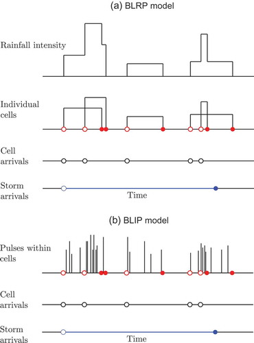
In the basic Bartlett-Lewis Rectangular Pulse (BLRP) model, storms arrive in a Poisson process of rate λ, each storm generating a cluster of cell arrivals. The Bartlett-Lewis clustering mechanism assumes that the time intervals between successive cells are independent, identically distributed random variables (whereas in the Neyman-Scott model, it is the temporal distances of the cells from their storm origin that are independent and identically distributed). It is normally assumed that the intervals between cells are exponentially distributed, so that the cell arrivals constitute a secondary Poisson process of rate β. Each cell is associated with a rectangular pulse of rain, of random duration, L, and with random intensity, X. In the simplest version of the model, these are both assumed to be exponentially distributed with parameters η and 1/µ_X, respectively, and are independent of each other. The cell origin process terminates after a time that is also exponentially distributed with rate γ. This basic version thus has five parameters in total. Both storms and cells may overlap, and the total intensity of rain at any point in time, Y(t), is given by the sum of all pulses ‘active’ at time t.

The process in respect of a single storm is illustrated in Fig. 1(a). Additional flexibility can be added by allowing for a distribution with more parameters for pulse intensities. A distribution with a longer tail may help in particular with the fit of extreme values, and popular variants include the Gamma, Weibull and Pareto distributions. One additional parameter is required in order to use either of these.

Fig. 1 Illustration of a single storm; storm and cell origins are denoted by open circles, and terminations by filled circles. In the BLRP model, each rain cell is assumed to have a constant intensity, whereas in the BLIP model, each cell consists of a series of instantaneous pulses.

In order to allow for different types of rainfall, multiple superposed processes can be used (Cowpertwait 2004, Cowpertwait et al. 2007). Due to parameter identification issues, the number of processes is typically limited to just two, which can be thought of as representing heavy, short-duration convective and lighter, long-duration stratiform types of rainfall. However, a potentially more parsimonious approach to enable variation between storms is to randomize the cell duration parameter and related temporal storm characteristics. The Random Parameter Bartlett-Lewis (BLRPR) model (Rodriguez-Iturbe et al. 1988) extends the basic model by allowing the parameter η, that specifies the duration of cells, to vary randomly between storms. This is achieved by assuming that the η values for distinct storms are independent, identically-distributed random variables from a gamma distribution with index α and rate parameter ν. The model is re-parameterized so that, rather than keeping the cell arrival rate, β, and the storm termination rate, γ, constant for each storm, it is the ratio of both of these parameters to η that is kept constant. Thus, for a higher η (i.e. typically shorter cell durations), we have correspondingly shorter storm durations, and shorter cell inter-arrival times. Essentially, the effect is that all storms have a common structure, but distinct storms occur on different (random) time-scales.

The durations of cells and storms (more precisely cell origin processes) are both exponentially distributed, conditional on the cell duration parameter, η. Their unconditional distributions are Pareto type II. This heavy-tailed distribution has an infinite mean if α is less than 1, and an infinite variance if α is less than 2. Also, in terms of the aggregated rainfall process, it turns out that, for values of α smaller than 3, the variance is infinite, and for values smaller than 4, the skewness is infinite. This is potentially problematic. For example, in practice it has been found that simulations with unconstrained values of α occasionally generate unrealistically long periods of rainfall (Onof and Arnbjerg-Nielsen 2009, Verhoest et al. 2010). This can be addressed by setting constraints on α, or rejecting storms or cells beyond a certain length or cells with an excessive intensity within any simulations. Alternatively, the gamma distribution for the cell duration parameter, η, may be truncated, with support (ε, ∞) (Onof and Arnbjerg-Nielsen 2009). The lower limit, ε, for the integrals over η can be pre-specified, or, alternatively, can constitute a further parameter to be determined.

The Bartlett-Lewis Instantaneous Pulse (BLIP) model (Cowpertwait et al. 2007), intended for fitting to fine-scale (of the order of 5- to 15-min) data, has a minimum of six parameters (one more than the original Bartlett-Lewis model) and is illustrated in Fig. 1(b). As in the BLRP model, storm origins arrive in a Poisson process of rate λ, and each storm origin initiates a Poisson process of cell origins of rate β. In contrast to the basic Bartlett-Lewis model, however, it is not assumed that there is a cell at the storm origin itself, so a storm may have no rainfall. This is purely for mathematical convenience and does not lead to any loss of generality. Each cell origin initiates a further Poisson process of rainfall pulses of rate ξ. Again, it is not assumed that there is a pulse at the cell origin, so a cell may have no rainfall. Note that the pulses are instantaneous: they have a depth, but no duration. This Poisson process of instantaneous pulses replaces the rectangular pulse assumption of the original Bartlett-Lewis model. Both the storm duration (the duration of the cell origin process) and the cell duration are assumed to be exponentially distributed, the former with rate γ, and the latter with rate η. The process of pulses terminates with the cell or storm lifetime, whichever is the sooner. Associated with each pulse is a depth, X, so the pulse process is a marked point process (Cox and Isham 1980). The model developed by Cowpertwait et al. (2007) allows pulse depths from a single cell to be dependent, but those from distinct cells are assumed independent. No specific dependence structure is specified, and the model fitted in the paper assumed independent, exponentially distributed pulse depths, with mean depth µ_X. Cowpertwait et al. (2007)’s model also assumed two superposed processes, with a common depth parameter across the two storm types, giving a total of eleven parameters.

2.2 Development of the Random Parameter Bartlett-Lewis Instantaneous Pulse (BLIPR) model

For the randomization of η in the BLIP model, we take the same approach as for the original Bartlett-Lewis model, but now with the additional assumption that the ratio (ω = ξ/η) of the pulse arrival rate to the cell duration parameter is kept constant.

In order to calculate the moments, it is helpful to think of the random parameter model as the superposition of a continuum of independent processes with random cell duration parameter, η, and storm origin rate, λf (η), where f (η) is the density function of η. Now, the rth cumulant of a sum of independent random variables is the sum of their rth cumulants. Therefore the mean, variance and 3rd central moment (which are the first three cumulants) can simply be obtained by replacing λ with λ f (η) in their original equations, and integrating over possible values of η.

The integration approach described requires some expectations of functions of η. In particular, we need:

for k = 1 and various values of x, given by:

(1)

Note that, in order for the integral not to diverge at zero, we require α > k. This proved to be an issue for the original Bartlett-Lewis model, as discussed in Section 2.1, where the skewness integral included elements with k = 4. For the BLIPR model, we only require α > 1 in order for the integrals for the variance and skewness of the aggregated rainfall not to diverge. However, the constraint α > 2 may still be desirable (or a ‘truncated’ version used) in order to prevent the simulation of unrealistically long rain events, as discussed.

The moments are derived from the original equations of Cowpertwait et al. (2007) by taking expectations over η and using the formula above. As in the original fixed parameter BLIP model, the flexibility to allow pulse depths to be dependent within cells is retained. In their empirical fits, Cowpertwait et al. (2007) assumed these to be independent, but, intuitively, dependent pulse depths should allow higher values of extremes at short time-scales. This is desirable since the fits understated 5-min extreme values. The moments for the new model are given in Appendix A.

3 FITTING METHODOLOGY

The generalized method of moments (GMM) is used for fitting. This is an extension of the method of moments which estimates parameters by equating expressions for population moments with their sample values. In the GMM, the number of properties to be fitted exceeds the number of unknown parameters, and the estimator is given by the value of θ that minimizes:

(2)

for some positive definite weighting matrix W, where θ is the unknown parameter vector, T is the vector of observed values for a set of k properties, and τ(θ) is the vector of their expected values under the model. The term S is referred to as the ‘objective function’. The optimal weights matrix (in terms of the identifiability of parameters) is the inverse of the covariance matrix of statistics (Hansen 1982), which here must be estimated empirically due to the complexity of the analytical expressions. In a recent simulation study using a point process based rainfall model, Jesus and Chandler (2011) find that a two-step approach is required in order to derive a reliable sample estimate of the full covariance matrix, but that the diagonal matrix of inverse variances, calculated using just a single step, is close to optimal, and this is the approach that we follow. The objective function becomes:

(3)

with w_i equal to 1/var(T_i(y)). Variances are calculated separately for each calendar month, pooling the data over observation years, and a separate fit is then produced for each month to allow for seasonality.

Note that, since the number of properties included in S exceeds the number of parameters, there is no guarantee that there will be a good fit to all the fitting properties. The adequacy of the fit is thus assessed by considering properties used in the fitting procedure, as well as others that are of interest in hydrological applications. Some properties will need to be assessed using simulations, for example, extreme values.

We follow Cowpertwait et al. (2007) in our choice of fitting properties – the hourly mean, plus the coefficient of variation, lag-1 correlation and skewness at time-scales of 5 min, 1 h, 6 h and 24 h.

Minimization of S requires a numerical optimization routine. The approach followed here is that of Wheater et al. (2005), and we have used the optimization routines developed for that project. Firstly, a set number of optimizations are carried out using the Nelder-Mead method, each starting with a different initial value for the set of parameters. This set of initial values is generated by random perturbation about a single user-supplied value. The best parameter set is then used as a new starting value for a further set of optimizations, which now use a Newton-type algorithm. The reason for the use of two different optimization routines is that the first is more robust and thus well suited to identifying promising regions of the parameter space, whereas the second is more powerful if given good starting values.

Different approaches to estimating parameter uncertainty have been taken in the literature. Rodriguez-Iturbe et al. (1988) look at parameter stability for the random parameter Bartlett-Lewis model by perturbing the input statistics by small amounts (±2%) and looking at the impact on the resulting parameter estimates. Cowpertwait (1998) uses a bootstrap approach, obtaining 100 sets of parameter estimates by fitting a Neyman-Scott model 100 times, each time using whole years sampled with replacement from the series of observed data. Sampling whole years (separately for each calendar month) ensures that the dependencies in the rainfall series are captured. Wheater et al. (2005) outline a method, based on the asymptotic theory of estimating equations, to estimate standard errors. Another approach, used by Chandler (2003), is the examination of profile objective functions, which is our preferred method here. Each parameter in turn is fixed at each of a set of values, and the objective function is optimized over the remaining parameters. The resulting plot for each parameter showing the optimized objective function against the set of parameter values provides a useful means for assessing the identifiability of the parameter—for example, a very flat objective function indicates a wide range of plausible values. If the optimal weighting matrix is used, it can be shown that has a distribution, where θ_p is a single component of the parameter vector, θ, and ψ is the vector of remaining parameters, and this result can be used to calculate approximate 95% confidence intervals for each parameter. Although this result does not hold if a non-optimal weighting matrix is used, a useful approximation has been suggested by Jesus and Chandler (2011).

4 COMPARISON OF MODELS ON BOCHUM DATA

4.1 Models fitted

The models were fitted, using the methodology and fitting properties discussed, to 69 years of five-minute rainfall data from a single site in Bochum in Germany. In each case, we assume that σ_X/µ_X = 1, and that (consistent with X being exponentially distributed). Initially, no further constraints were imposed on the parameters, other than that they should be greater than zero. The six models initially fitted were as follows:

Rectangular pulse models

1. the Bartlett-Lewis Rectangular Pulse model (BLRP)

2. the Random Parameter Bartlett-Lewis Rectangular Pulse model (BLRPR)

3. the Bartlett-Lewis Rectangular Pulse model with two superposed processes (BLRP2)

Instantaneous pulse models

1. the Bartlett-Lewis Instantaneous Pulse Model (BLIP)

2. the Random Parameter Bartlett-Lewis Instantaneous Pulse model, introduced in Section 2.2 (BLIPR)

3. the Bartlett-Lewis Instantaneous Pulse model with two superposed processes (BLIP2).

For the Bartlett-Lewis Rectangular Pulse model, on randomizing the cell duration parameter η, the fitted solution gave such a high precision to the mean cell duration, that it effectively replicated the non-random solution. Thus, the fitted parameter set for the BLRPR model is simply a re-parameterized version of the set of BLRP parameters, and there is thus no improvement in the fit compared with the fixed η version. This appears to contradict examples in the literature where the randomized η version had shown an improved fit compared to the fixed η model (Rodriguez-Iturbe et al. 1988, Wheater et al. 2005). On further investigation, we concluded that the improvement in the fit to proportion dry that had previously been found by randomizing η was at the expense of a deterioration in the fit to the skewness, which had not been included as a fitting property in these earlier analyses. In particular, if skewness is not included in the fit, it is highly overestimated in the summer months at time-scales of 6 and 24 h.

Fitting the models with two superposed processes proved problematic. Although the BLRP2 model with no parameter constraints gave a very good fit in terms of a low minimum objective function value, the parameters thus obtained were highly unstable, unrealistic and inconsistent from month to month, and no standard errors could be found. It was clear that there was insufficient information in our observed data to identify the large number of required parameters. Introducing constraints for the parameters increased the minimum objective function values, and did not resolve the situation, with resulting solutions having many parameters lying on the constraint boundaries. We therefore concluded that ensuring realistic and reasonably smooth parameters across months would require constraints on the relationships between parameters, rather than just setting bounds on individual parameters. There were similar issues with the BLIP2 model. Ultimately we decided that both of these models’ parameter identifiability issues made them unsuitable for practical application, at least in the context of this dataset and set of fitting properties, and our requirement for a model that is robust and easy to fit.

Given the above findings, we present further results here for the following three models only: BLRP, BLIP and BLIPR.

For the BLIP and BLIPR models we initially followed Cowpertwait et al. (2007) and assumed that pulses within a single cell had independent depths. However, for the BLIPR model an alternative assumption was also considered, whereby pulses within a single cell have a common depth (the most extreme form of dependence). The latter achieved a lower minimum objective function value in all months, and a better fit in respect of properties not included in the fitting process, such as wet/dry properties. For both of these options, the unconstrained solution gave an extremely high number of pulses per hour (of the order of 10⁵–10⁶), so for practical reasons, was constrained to be 0.001, reducing the number of parameters by one. All other fitted parameters were broadly as before, except for a corresponding change in ω. The quality of the fit was unchanged with this constraint, as the product term effectively forms a single composite parameter over most of the possible parameter space. We also considered two alternative constraints on α: α > 1 or α > 2, as discussed in Section 2.2. The former only affects July, whereas the latter affects all the summer months.

A comparison of the performance of the three fitted models, together with the findings discussed earlier in this section and consideration of the fitted parameter sets (shown in Appendix B, Tables B1–B3) led us to a hypothesis, which we present in the next section.

4.2 Initial performance comparison of the fitted models

Table 1 shows the minimum objective function value for each of the models that we have successfully fitted, for each month. Since the same set of moments and weights were used for each model, these are directly comparable.

Key findings from the results are summarized below:

• The BLRP model outperforms the BLIP model, with a lower minimum objective function value in all months except January and December. The model with rectangular pulses has generally been considered unsuitable for time-scales shorter than the mean cell duration, due to the unrealistic intensity shape. However, when fine-scale data are available for fitting, the fitted model tends to have shorter, more frequent cells than if only hourly data are available (of the order of 5–10 min, compared with 20–40 min for most months), which are still within a realistic range. With these shorter cells, and given also the potential for cells to overlap, repetition of the same rainfall totals over consecutive 5-min intervals is relatively infrequent. The fitted parameters are shown in Appendix B (Table B1), along with some key properties such as mean storm and cell inter-arrival times and durations.

• When skewness is included in the fit, there is no benefit to randomizing the cell duration parameter in respect of the BLRP model, as discussed in Section 4.1. However, there is a clear benefit in respect of the BLIP model, with the randomized version showing the best performance of all the models.

• The fitted BLIPR model has a very high number of pulses per cell (particularly if we do not apply constraints, as discussed), with very short inter-arrival times, and the better performing version has common within-cell pulse depths. Effectively then, the cells are ‘rectangular’.

These results imply that it is not the replacement of rectangular pulses by clusters of instantaneous ones that leads to the improved performance of the BLIPR model, compared with the BLRPR model. Instead, the improved performance can be attributed to the fact that the BLIPR model allows rainfall intensity to vary with cell duration, since the pulse rate effectively drives the intensity and is proportional to the cell duration parameter, η. Our new model variant thus gives a simple, but effective way of introducing dependence between cell duration and intensity.

This suggests that the same effect could be achieved by amending the BLRPR model, so that the mean cell intensity parameter, µ_X is also varied in proportion to the cell duration parameter, η. This is preferable from a computational point of view, eliminating the need for simulation of a vast number of instantaneous pulses.

4.3 Testing our hypothesis and new model variant

Extending the BLRPR model to allow µ_X to vary in proportion to the cell duration parameter, η, is straightforward, and follows the methodology discussed in Section 2.2. We re-parameterize the BLRPR model so that the ratio, ι = µ_X/η is now kept constant, and express E(X²) and E(X³) in terms of ι also (for which the formulae depend on the choice of distribution for the rainfall intensity). We then take expectations over η as before. The analytical expressions for this new model, which we denote the BLRPR_X model, are given in Appendix A.

The fitted parameter set, assuming an exponential distribution for cell intensities as before, is given in Table B4 (Appendix B). Comparing this with the fitted parameters of the Random Parameter Bartlett-Lewis Instantaneous Pulse (BLIPR) model with common within-cell pulse depths, shown in Table B3, the strong similarity between the two models is evident. In particular, the new parameter, ι, of the BLRPR_X model broadly equates to µ_X ω of the BLIPR model (noting that µ_X represents an intensity in the rectangular pulse models, but a depth in those with instantaneous pulses). Values of the minimum objective function (see Table 2) and plots of the two fits are also found to match, thus supporting our hypothesis.

We have therefore established that the new rectangular pulse model variant is effectively equivalent to the BLIPR model with common within-cell pulse depths, and that there is therefore no need to replace the rectangular pulses with a process of instantaneous pulses for fine-scale data. This is the optimal model, at least in terms of the minimum objective function values. In the next section we examine the performance of the three models (BLRP, BLIP, BLRPR_X) in more detail, firstly in terms of the fitted moments, and then by considering wet/dry properties, which were not included within the objective function, and extreme value performance.

4.4 Performance comparison of the fitted models

4.4.1 Fitted moments

Plots of the fits of the models (BLRP, BLIP, BLRPR_X) against the observed data for each month in respect of the mean, coefficient of variation, lag-1 autocorrelation and skewness coefficient are shown in Figs 2–5. Note that the y-axes for these and other similar plots in this paper have been selected automatically such that, for each individual plot, the axis spans the range covered by the observed and fitted values. This means that the fit in respect of an individual model tends to look worse if all models fit well, than if at least one of the other plotted models has a poor fit (since in the latter case the scale will be wider). Care should therefore be taken to consider also the scale when examining such plots.

Fig. 2 Mean 1-hour rainfall by month, fitted vs observed.

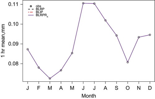
Fig. 3 Coeffient of variation by month, fitted vs observed.

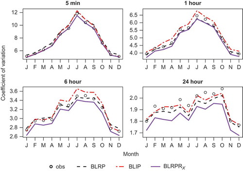
Fig. 4 Lag-1 autocorrelation by month, fitted vs observed.

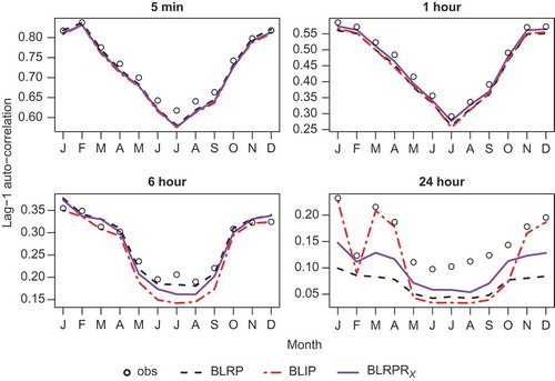
Fig. 5 Coeffcient of skewness by month, fitted vs observed.

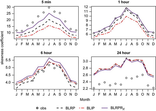
All the models generally perform well with respect to the properties included in the fitting. They reproduce the mean exactly (this is not a given, since the number of properties fitted exceeds the number of parameters), and fit the coefficient of variation well at all time-scales. All tend to underestimate the lag-1 autocorrelation at longer time-scales. All also tend to underestimate the skewness at the shorter time-scales, with the BLRPR_X model showing the best fit in respect of 5-min skewness, and the BLIP model the worst.

4.4.2 Wet/dry properties

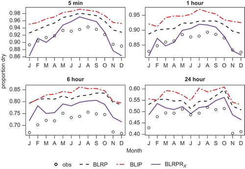
The proportion of dry intervals is a very important property for hydrological applications. Although this could have been included as one of the fitting properties, it is useful to reserve an important feature for subsequent model validation, as this gives an independent test of the appropriateness of the model structure. Plots of the fits of the models against the observed data for each month in respect of the proportion dry are shown in Fig. 6. The BLRPR_X model can be seen to outperform the other models with respect to the fit to proportion dry, across all time-scales.

Fig. 6 Proportion of intervals that are dry by month, fitted vs observed.

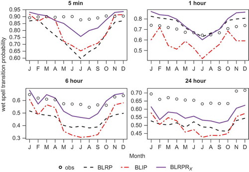
It is also of interest to consider the wet and dry spell transition probabilities (i.e the probability that a wet interval is followed by another wet interval, or a dry by another dry), which are important for the accurate modelling of antecedent conditions. Fig. 7 shows that the BLRPR_X model again outperforms the other models with respect to the wet spell transition probability. While the BLRP model has a good fit at the hourly time-scale, it performs poorly at other time-scales, with only the BLRPR_X model showing consistency of performance across time-scales. There is less difference between models for the dry spell transition probabilities, with all models providing a reasonable fit at all time-scales. The fit to the wet/dry properties in respect of the summer months would be further improved if we did not impose the constraint that α > 2. However, this would be at the expense of allowing storms and cells of unrealistic durations in the simulations (as discussed in Section 2.2), and also a slight deterioration of the fit to the 24-h variance, and 6-h lag-1 autocorrelation.

Fig. 7 Transition probability of a wet interval being followed by another wet interval, by month, fitted vs observed.

4.4.3 Extreme value performance

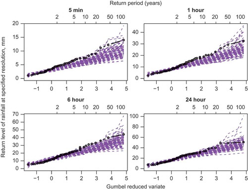
For our data, the months with the highest rainfall, rainfall variability and skewness are the summer months, and these are also the months with the highest extremes. A comparison of the fit of extremes for July for the BLRPR_X model is given in Fig. 8, using Gumbel plots. We use 100 simulations, allowing for parameter uncertainty by sampling from the distribution of the parameter set for each simulation, which is of the same length as the observed data. The maximum rainfall per unit-time is plotted against the ‘reduced-variate’ −ln(−ln(1 − 1/R)), where R is the return period. The graphs for July show that the model has a tendency to underestimate extremes, as has been noted before for this type of model. Results for other months give a fairly similar picture.

Fig. 8 Gumbel plots of observed (black) vs simulated (purple) extremes for July, using the BLRPR_X model and 100 simulations, each of 69 years; α constrained to be greater than 2.

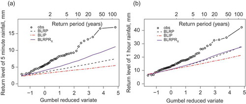
A comparison showing mean annual extremes (averaged over 50 simulations) for a number of alternative models at the 5-min and hourly time-scales is also shown in Fig. 9. At the 5-min time-scale, the BLRPR_X model gives the best performance, although all the models underestimate the extremes. Results are closer at the 1-h time-scale, and for longer time-scales, there is essentially no difference between models.

Fig. 9 Annual Gumbel plots of observed vs simulated extremes for variants of the Bartlett-Lewis model, at (a) 5 min and (b) hourly time-scales.

Based on our analysis, the BLRPR_X is shown to be the best performing of the models compared, both in terms of the moments fitted, and more importantly, in respect of the wet/dry properties and extreme values, neither of which is included in the fit. It is also intuitively appealing, since the intensity of rainfall is known to vary inversely with the duration of the rain event. Further, this dependence has been introduced to the BLRPR model without the need for any additional parameters or complexity. Considering the fitted parameter set, shown in Table B4 (Appendix B), the parameter values change fairly smoothly from month to month. Comparing with empirical observations from Houze and Hobbs (1982), the parameter values seem reasonable. Winter storms last several hours, have around 20 cells, which each last on average around 22 min. In summer, storms and cells are shorter, and have around eight cells. However, these have a correspondingly much higher intensity, giving broadly the same amount of rainfall per storm over all months.

5 PARAMETER IDENTIFIABILITY AND CONFIDENCE INTERVALS

Finally, we explore the parameter identifiability of the new BLRPR_X model using profile objective functions as described in Section 3. Profile objective functions for the logarithm of the parameters are shown in Fig. 10 for the month of January. As before, we have constrained the value of α to be greater than 2 (except in the plot for α itself). The first set of plots shows a wide range of possible parameter values, allowing us to check whether there are multiple local minima, for example, or extensive regions where the objective function is flat. We have then reduced the parameter range so that the approximate 95% confidence intervals can be seen more clearly. The plots show that the parameters are fairly well identified in January. Results for other months (not shown) again indicate good parameter identification, although there is slightly more parameter uncertainty in the summer months, which is fairly typical.

Fig. 10 Profile objective function plots for the BLRPR_X model for January; the plots show the logarithms of the parameters, for (a) wide parameter range and (b) reduced parameter range.

6 POTENTIAL FURTHER IMPROVEMENTS

Although the new model fits well, there are areas for improvement, the most important of which is the fit to extreme values, which are understated. This is perhaps surprising, as intuitively the inclusion of the skewness coefficient as one of the fitting properties should lead to an improved fit in respect of extremes. On investigation, we found that our approach of averaging the skewness over 69 separate observation months, rather than calculating a single statistic over the whole of the data, tends to understate the skewness coefficient itself, particularly at the 5-min time-scale. This is found to be related to the effective weights that are applied to periods of high skewness under the two alternative approaches, rather than to sampling variation, or to the choice of mean (local or global) about which the moments are centred. The alternative approach would have given us a slightly better fit to extremes, but does not permit the calculation of the covariance matrix for the observed statistics, since it is just a single sample.

It is generally thought that a distribution for the rainfall intensity with ‘fatter tails’ should improve the fit to extremes. This was investigated by replacing the exponential distribution with the gamma and Weibull distributions, both of which have the exponential as a special case. The Weibull distribution gave the better performance here. However, the addition of a further parameter caused problems in terms of parameter identifiability, with less consistency from month to month. Also the asymptotic results showed a very high correlation between the estimated shape parameter and the intensity parameter, suggesting that an additional parameter is not justified. Constraining the shape parameter to a fixed value may, however, be a viable strategy, since this does not require any additional parameters. Here the fitted shape parameter was close to 0.6 in most months. Using a Weibull conditional intensity distribution with a shape parameter of 0.6 rather than an exponential (which has a shape parameter of 1) improves the fits to 5-min skewness and to extremes at short time-scales, but with some deterioration in the lag-1 autocorrelation at longer time-scales.

Another alternative considered for the BLRPR_X model involved allowing a more flexible intensity/duration relationship, by letting the mean intensity be proportional to the cell duration parameter, raised to some fixed power, the level of which is to be determined, i.e. to have ι = µ_X/η^c for some additional parameter, c. However, it was found that the fitted values of c were fairly close to 1, suggesting that this additional complexity is not required. Alternative formulae for this relationship could be considered, but are likely to affect the analytical tractability.

7 DISCUSSION AND CONCLUSIONS

In this paper, using a structured comparison of different versions of the Bartlett-Lewis clustered point process-based models, including two new model extensions, we have clarified some key aspects of performance. Our focus here has been on fine scale data. We have highlighted some limitations in all the models, notably an inability to achieve a good fit to all properties in the summer months of a temperate climate, when rainfall exhibits particularly high variability and skewness. Such limitations are not surprising when we consider the simplicity of these models compared with the highly complex real physical rainfall process. The challenge of achieving a good fit at time-scales that cover the wide range from five minutes up to daily, is particularly demanding. However, the performance of the original rectangular pulse (BLRP) model, originally considered unsuitable for fine-scale data due to the unrealistic rectangular pulses, has far exceeded prior expectations.

We showed that the main driver behind improved performance, particularly in respect of skewness and extremes at short time-scales, is the introduction of an inverse dependence between rainfall intensity and cell duration. Our proposed new model, which is an extension of the Random Parameter Bartlett-Lewis Rectangular Pulse model, gives a simple but effective way of introducing such dependence, with no increase in the number of parameters. It allows the rainfall intensity parameter, µ_X, previously assumed to be constant, to vary in proportion to the cell duration parameter, η, which itself varies randomly between storms. Although instantaneous pulses were useful in leading us to this conclusion, ultimately we discovered that they are not required, and the computationally simpler rectangular pulse version is preferred. Adding further parameters adds little to the fit, since typically improvements in some properties cause degradation in others, and more parameters bring issues of parameter identifiability and consistency. Replacing the exponential intensity distribution with a Weibull with a fixed shape parameter, however, may be desirable. The introduction of depth-duration dependence is desirable for all datasets and time-scales, although the positive impact of the new model is greatest for fine-scale data.

Appropriately allowing for the uncertainty in the parameter estimates is important, and this is often not addressed in the hydrological literature. A suggested approach, used here when generating simulations, is to sample parameters from the asymptotic multivariate normal distribution (or lognormal if the logarithms of the parameters are fitted). In this way, rare, but potentially damaging scenarios should be better represented in simulations, particularly if, as here, extreme values tend to be underestimated by the model.

Funding

Jo Kaczmarska is pleased to acknowledge financial support from the Engineering and Physical Sciences Research Council.

Acknowledgements

Deutsche Montan Technologie and Emschergenossenschaft/Lippeverband in Germany are gratefully acknowledged for providing the data. We would also like to thank Richard Chandler and Joao Jesus for helpful advice.

APPENDIX A

FORMULAE FOR FITTING PROPERTIES

In Appendix A, we give the formulae for the mean, variance, lag-1 autocovariance and third central moment of the discrete-time aggregated process in respect of the BLIPR and BLRPR_X models. Throughout, the time-scale to which the continuous process is aggregated is denoted as h. The required fitting properties can be derived from those given here, as follows:

(A1)

(A2)

(A3)

The random cell intensity, denoted X, has been assumed to have a one parameter distribution. The parameterization in respect of the Exponential distribution, used here, is as follows:

Parameter : µ_X

Moments : E(X) = µ_X E(X²) = 2µ²

A1 MOMENTS FOR THE BARLETT-LEWIS INSTANTANEOUS PULSE RANDOM η (BLIPR) MODEL

Parameter definitions

• λ - storm arrival rate

• α - shape parameter for the Gamma distribution of the cell duration parameter, η

• ν - scale parameter for the Gamma distribution of η

• κ - ratio of the cell arrival rate to η (i.e. β/η)

• φ - ratio of the storm (cell process) termination rate to η (i.e. γ/η)

• ω - ratio of the pulse arrival rate to η (i.e. ξ/η)

• µ_X - mean pulse depth

• E(X²) - mean of squares of pulse depths

• E(X³) - mean of cubes of pulse depths

• E(X_ijk X_ijl) - product moment of the depths of 2 pulses within the same cell

• E(X_ijk X_ijl X_ijm) - product moment of the depths of 3 pulses within the same cell

• - mean number of pulses per storm

Mean

(A4)

Variance

(A5)

Covariance at lag

(A6)

Third central moment

(A7)

A2 MOMENTS FOR THE RANDOM PARAMETER BARTLETT-LEWIS RECTANGULAR PULSE MODEL WITH DEPENDENT INTENSITY–DURATION (BLRPR_X)

All expectations are left in the form for various values of k and s, and may be evaluated as:

Parameter definitions

• λ - storm arrival rate

• α - shape parameter for the Gamma distribution of the cell duration parameter, η

• ν - scale parameter for the Gamma distribution of η

• κ - ratio of the cell arrival rate to η (i.e. β/η)

• φ - ratio of the storm (cell process) termination rate to η (i.e. γ/η)

• ι - ratio of mean cell intensity to η (i.e. µ_X /η)

• =

• =

• µ_C = 1 + κ/φ - mean number of cells per storm

Mean

(A8)

Variance

(A9)

Covariance at lag

(A10)

Third central moment

(A11)

APPENDIX B

FITTED PARAMETERS

For each model, as well as the fitted parameters, we show a number of key properties, in order to allow a better comparison of models with different parameterizations. The acronyms used for these properties are given below:

• MSIT mean storm inter-arrival time (h)

• MSD mean duration of storm activity (h)

• MCIT mean cell inter-arrival time (min)

• MCD mean cell duration (min)

• MCS mean number of cells per storm (= µ_C)

• MPC mean number of pulses per cell

Table B1 Parameters for BLRP model.

	λ	µX	β	γ	η	MSIT	MSD	MCIT	MCD	MCS
Jan	0.022	0.960	5.422	0.231	5.975	45.0	4.3	11.1	10.0	24.5
Feb	0.021	0.942	5.142	0.260	5.310	47.1	3.8	11.7	11.3	20.7
Mar	0.021	1.334	4.478	0.262	7.061	47.2	3.8	13.4	8.5	18.1
Apr	0.022	1.944	3.829	0.271	8.387	45.7	3.7	15.7	7.2	15.1
May	0.023	3.662	3.157	0.370	9.239	44.3	2.7	19.0	6.5	9.5
Jun	0.025	6.431	2.694	0.413	11.154	39.2	2.4	22.3	5.4	7.5
Jul	0.023	10.136	1.672	0.356	12.011	43.5	2.8	35.9	5.0	5.7
Aug	0.023	7.072	2.411	0.408	11.066	43.4	2.5	24.9	5.4	6.9
Sep	0.021	5.306	2.945	0.379	10.470	47.1	2.6	20.4	5.7	8.8
Oct	0.019	2.209	4.071	0.275	8.104	53.3	3.6	14.7	7.4	15.8
Nov	0.023	1.207	5.884	0.276	6.741	42.8	3.6	10.2	8.9	22.3
Dec	0.024	1.059	5.475	0.265	5.906	41.1	3.8	11.0	10.2	21.7

Table B2 Parameters for BLIP model, with independent within-cell pulse depths.

	λ	µX	β	γ	η	ξ	MSIT	MSD	MCIT	MCD	MCS	MPC
Jan	0.023	0.013	0.220	0.078	1.166	124.9	43.0	12.9	272.2	51.5	2.8	100
Feb	0.025	0.008	1.387	0.239	2.547	182.7	39.7	4.2	43.3	23.6	5.8	66
Mar	0.022	0.020	0.188	0.079	1.393	97.8	44.7	12.7	319.8	43.1	2.4	66
Apr	0.024	0.033	0.209	0.094	1.684	77.3	41.0	10.7	287.6	35.6	2.2	43
May	0.028	0.038	1.452	0.420	5.696	144.1	35.8	2.4	41.3	10.5	3.5	24
Jun	0.033	0.086	1.237	0.488	6.101	100.8	30.0	2.1	48.5	9.8	2.5	15
Jul	0.032	0.141	0.707	0.423	6.558	100.9	30.8	2.4	84.9	9.1	1.7	14
Aug	0.031	0.095	1.042	0.477	6.023	103.2	32.2	2.1	57.6	10.0	2.2	16
Sep	0.027	0.068	1.355	0.442	5.826	105.3	37.1	2.3	44.3	10.3	3.1	17
Oct	0.021	0.022	1.652	0.282	4.758	145.8	46.5	3.6	36.3	12.6	5.9	29
Nov	0.029	0.018	0.237	0.107	1.208	107.4	34.8	9.4	253.0	49.7	2.2	82
Dec	0.028	0.014	0.213	0.093	1.183	129.4	35.2	10.8	281.4	50.7	2.3	101

Table B3 Parameters for BLIPR model, with common within-cell pulse depths; constraints: .

	λ	µX	α	α/ν	κ	φ	ω	MSIT	MSD	MCIT	MCD	MCS	MPC
Jan	0.024	0.001	2.147	4.591	1.027	0.046	173	42.3	8.9	23.8	24.5	22.4	165
Feb	0.023	0.001	3.680	4.394	1.096	0.058	187	42.6	5.4	17.1	18.8	18.8	177
Mar	0.023	0.001	2.000	5.525	0.712	0.043	204	44.1	8.3	30.5	21.7	16.4	195
Apr	0.024	0.001	2.000	6.740	0.517	0.039	248	41.7	7.7	34.4	17.8	13.4	239
May	0.027	0.001	2.000	7.760	0.437	0.054	413	37.3	4.8	35.4	15.5	8.1	392
Jun	0.031	0.001	2.000	9.607	0.310	0.050	606	32.1	4.1	40.3	12.5	6.2	576
Jul	0.030	0.001	2.000	10.413	0.167	0.039	908	33.4	4.9	69.2	11.5	4.2	874
Aug	0.029	0.001	2.000	9.683	0.293	0.053	663	34.4	3.9	42.2	12.4	5.6	630
Sep	0.025	0.001	2.000	8.901	0.345	0.047	534	40.1	4.8	39.1	13.5	7.4	510
Oct	0.021	0.001	2.126	6.698	0.580	0.041	286	48.4	6.9	29.2	16.9	14.3	274
Nov	0.025	0.001	2.000	5.389	1.055	0.049	182	39.9	7.6	21.1	22.3	21.5	173
Dec	0.026	0.001	2.035	4.584	1.093	0.054	188	37.9	7.9	23.6	25.7	20.1	179

Table B4 Parameters for BLRPR_X model, with dependent intensity/duration (); constraint:

	λ	ι	α	α/ν	κ	φ	MSIT	MSD	MCIT	MCD	MCS
Jan	0.022	0.164	2.075	5.014	0.996	0.042	46.2	9.1	23.2	23.1	24.6
Feb	0.021	0.177	3.451	4.818	1.063	0.053	47.5	5.5	16.5	17.5	20.9
Mar	0.020	0.196	2.000	5.910	0.695	0.041	48.8	8.3	29.2	20.3	18.0
Apr	0.022	0.241	2.000	7.083	0.509	0.037	46.5	7.6	33.3	16.9	14.8
May	0.023	0.400	2.000	8.127	0.434	0.052	43.9	4.7	34.0	14.8	9.4
Jun	0.026	0.586	2.000	10.015	0.311	0.049	38.9	4.1	38.5	12.0	7.3
Jul	0.024	0.879	2.000	10.777	0.173	0.040	42.3	4.6	64.3	11.1	5.3
Aug	0.024	0.639	2.000	10.109	0.299	0.052	42.3	3.8	39.7	11.9	6.8
Sep	0.021	0.518	2.000	9.257	0.343	0.045	47.4	4.8	37.7	13.0	8.6
Oct	0.019	0.277	2.051	7.006	0.575	0.039	53.8	7.1	29.1	16.7	15.7
Nov	0.023	0.175	2.000	5.832	1.018	0.045	43.9	7.6	20.2	20.6	23.5
Dec	0.024	0.179	2.000	5.018	1.056	0.050	42.0	8.0	22.6	23.9	22.2

REFERENCES

- Burton, A., et al., 2010. Downscaling transient climate change using a Neyman-Scott Rectangular Pulses stochastic rainfall model. Journal of Hydrology, 381 (1–2), 18–32. doi:10.1016/j.jhydrol.2009.10.031
- Cameron, D., Beven, K., and Tawn, J., 2000. An evaluation of three stochastic rainfall models. Journal of Hydrology, 228, 130–149. doi:10.1016/S0022-1694(00)00143-8
- Chandler, R.E., 2003. Moment-based inference for stochastic-mechanistic models. Technical Report 7, DEFRA project FD2105. Improved Methods for national spatial-temporal rainfall and evaporation modelling for BSM.
- Cowpertwait, P.S.P., 1995. A generalized spatial-temporal model of rainfall based on a clustered point process. Proceedings of the Royal Society of London. Series A, Mathematical and Physical Sciences, 147–429.
- Cowpertwait, P.S.P., 1998. A Poisson-cluster model of rainfall: some high-order moments and extreme values. Proceedings of the Royal Society: Mathematical, Physical and Engineering Sciences, 454 (1971), 885–898. doi:10.1098/rspa.1998.0191
- Cowpertwait, P.S.P., 2004. Mixed rectangular pulses models of rainfall. Hydrology and Earth System Sciences, 8 (5), 993–1000. doi:10.5194/hess-8-993-2004
- Cowpertwait, P.S.P., 2010. A spatial-temporal point process model with a continuous distribution of storm types. Water Resources Research, 46 (12), W12507. doi:10.1029/2010WR009728
- Cowpertwait, P.S.P., et al., 2011. A fine-scale point process model of rainfall with dependent pulse depths within cells. Hydrological Sciences Journal, 56 (7), 1110–1117. doi:10.1080/02626667.2011.604033
- Cowpertwait, P., Isham, V., and Onof, C., 2007. Point process models of rainfall: developments for fine-scale structure. Proceedings of the Royal Society of London, Series A, 463 (2086), 2569–2587.
- Cox, D.R. and Isham, V., 1980. Point processes. London: Chapman and Hall.
- Hansen, L.P., 1982. Large sample properties of generalized method of moments estimators. Econometrica, 50 (4), 1029–1054. doi:10.2307/1912775
- Houze, R.A. and Hobbs, P.V., 1982. Organization and structure of precipitating cloud systems. Advances in Geophysics, 24, 225–315. doi:10.1016/S0065-2687(08)60521-X
- Jesus, J. and Chandler, R.E., 2011. Estimating functions and the generalized method of moments. Interface Focus, 1 (6), 871–885.
- Khaliq, M.N. and Cunnane, C., 1996. Modelling point rainfall occurrences with the modified Bartlett-Lewis rectangular pulses model. Journal of Hydrology, 180 (1–4), 109–138. doi:10.1016/0022-1694(95)02894-3
- Kilsby, C.G., et al., 2007. A daily weather generator for use in climate change studies. Environmental Modelling & Software, 22 (12), 1705–1719. doi:10.1016/j.envsoft.2007.02.005
- Moore, R.J. and Hall, M.J. eds., 2000. HYREX: the HYdrological Radar EXperiment. Hydrology and Earth System Sciences, 4 (4), 681 pp. Special issue.
- Onof, C., et al., 2000. Rainfall modelling using Poisson-cluster processes: a review of developments. Stochastic Environmental Research and Risk Assessment, 14, 384–411. doi:10.1007/s004770000043
- Onof, C. and Arnbjerg-Nielsen, K., 2009. Quantification of anticipated future changes in high resolution design rainfall for urban areas. Atmospheric Research, 92 (3), 350–363. doi:10.1016/j.atmosres.2009.01.014
- Rodriguez-Iturbe, I., Cox, D.R., and Isham, V., 1987. Some models for rainfall based on stochastic point processes. Proceedings of the Royal Society of London. Series A, Mathematical and Physical Sciences, 410, 269–288. doi:10.1098/rspa.1987.0039
- Rodriguez-Iturbe, I., Cox, D.R., and Isham, V., 1988. A point process model for rainfall: further developments. Proceedings of the Royal Society of London. Series A, Mathematical and Physical Sciences, 417, 283–298. doi:10.1098/rspa.1988.0061
- Smithers, J.C., Pegram, G.G.S., and Schulze, R.E., 2002. Design rainfall estimation in South Africa using Bartlett-Lewis rectangular pulse rainfall models. Journal of Hydrology, 258 (1–4), 83–99. doi:10.1016/S0022-1694(01)00571-6
- Vandenberghe, S., et al., 2011. A comparative copula-based bivariate frequency analysis of observed and simulated storm events: a case study on Bartlett-Lewis modeled rainfall. Water Resources Research, 47, W07529. doi:10.1029/2009WR008388
- Verhoest, N.E.C., et al., 2010. Are stochastic point rainfall models able to preserve extreme flood statistics? Hydrological Processes, 24 (23), 3439–3445. doi:10.1002/hyp.7867
- Verhoest, N., Troch, P.A., and De Troch, F.P., 1997. On the applicability of BartlettLewis rectangular pulses models in the modeling of design storms at a point. Journal of Hydrology, 202 (1–4), 108–120. doi:10.1016/S0022-1694(97)00060-7
- Wheater, H.S., et al., 2000. Generation of spatially consistent rainfall data. Report to the Ministry of Agriculture, Fisheries and Food (2 volumes). Department of Statistical Science, University College London. Research Report 204. Available from: http://www.ucl.ac.uk/Stats/research/reports [Accessed 13 August 2014].
- Wheater, H.S., et al., 2005. Spatial-temporal rainfall modelling for flood risk estimation. Stochastic Environmental Research and Risk Assessment, 19 (6), 403–416. doi:10.1007/s00477-005-0011-8