Statistical seasonal rainfall and streamflow forecasting for the Sirba watershed, West Africa, using sea-surface temperatures

ABSTRACT

The ability of various statistical techniques to forecast the July-August-September (JAS) total rainfall and monthly streamflow in the Sirba watershed (West Africa) was tested. First, multiple linear regression was used to link predictors derived from the Atlantic and Pacific sea-surface temperatures (SST) to JAS rainfall in the watershed up to 18 months ahead; then, daily precipitation was generated using temporal disaggregation; and finally, a rainfall–runoff model was used to generate future hydrographs. Different combinations of lag times and time windows on which SSTs were averaged were considered. Model performance was assessed using the Nash-Sutcliffe coefficient (E_f), the coefficient of determination (R²) and a three-category hit score (H). The best results were achieved using the Pacific Ocean SST averaged over the March–June period of the year, before the rainy season, and led to a performance of R² = 0.458, E_f = 0.387 and H = 66.67% for JAS total rainfall, and R² = 0.552, E_f = 0.487 and H = 73.28% for monthly streamflow.

Editor D. Koutsoyiannis; Associate editor Not assigned

KEYWORDS:

• seasonal forecasting
• sea-surface temperature
• canonical correlation analysis
• principal component analysis
• temporal disaggregation
• SWAT

1 Introduction

High inter-annual rainfall variability combined with an increase in aridity in the Sahel region of West Africa during the last three decades of the 20th century have been reported by several authors (Brooks 2004, Dai et al. 2004, Lu and Delworth 2005, Christensen et al. 2007, p. 871). Lu and Delworth (2005) reported a rainfall decrease of 20–50% in the region between 1950 and 2000. Samimi et al. (2012) reported exceptionally heavy precipitation with return periods of up to 1200 years during the 2007 rainy season in one Sahelian watershed. Both the drying and the variability are responsible for recurrent extreme (both low and high) precipitation levels that cause damage to several sectors of the local economy. The sector that is most often hit is rainfed agriculture, where productivity drops in the case of rain shortages, but irrigated agriculture can also be devastated by floods. Heavy precipitation in the Sahel received international media attention in 2007, 2008, 2009 and 2010 (Samimi et al. 2012). It was reported by IRIN (2012) that rice-growing fields along the River Niger and more than 7000 farms were flooded after heavy precipitation in August 2013.

The types of damage mentioned above occur mainly because the amount of rainfall or the peak water level in a given area happens to be too high or too low for the crops being cultivated. If information about the magnitude of the rains were available a few months before the rainy season, farmers could switch to a crop or a farm management scheme that is adapted to the upcoming rainy season. Therefore, any technique that can provide a hint about the upcoming rainy season a few months ahead of time might improve agricultural yields by increasing stakeholders’ level of preparedness. Such forecasts may be useful to many other water users, such as hydropower producers and municipalities relying on surface water for domestic and/or industrial consumption.

Seasonal forecasting, defined as the best available prediction of what climate will be like in the next few months, is a natural response to the problem. It is even considered an efficient approach to drought mitigation (Hayes et al. 2005). There are two main approaches to seasonal forecasting: (a) dynamical models, which are based on a relatively accurate simulation of the physical processes that drive the interactions between the atmosphere, land and ocean, and can account for the nonlinearities and feedback loops in these interactions; and (b) statistical models that rely on stationary relationships between predictors (usually sea-surface temperature, SST) and predictands (Schepen et al. 2012). Even though dynamical models are theoretically more likely to provide skillful forecasts (Palmer 1986, Marengo et al. 2003, Hansen et al. 2009), they are computationally intensive applications, and their output often has low temporal and/or spatial resolution, requiring an additional downscaling step for local impact studies (Wilby and Wigley 1997, Wetterhall et al. 2005, Busuioc et al. 2008). One major limitation of dynamical models is their coarse spatial resolution: since a few general circulation model (GCM) cells can cover an entire watershed, the spatial variability of climatic inputs is seriously diminished when GCM outputs are directly used as forcing variables. It is also known that GCMs have limited skill in resolving subgrid-scale features such as clouds, convection and topography (Xu 1999). For these reasons, downscaling is commonly applied to GCM simulation outputs (e.g. Landman et al. 2001, Charles et al. 2004, Raje and Mujumdar 2011). Therefore, statistical models are very popular in applications requiring higher temporal and spatial scales. One of these fields is streamflow forecasting.

Seasonal forecasts in the Sahel region are issued by two institutions: the African Centre of Meteorological Applications for Development (ACMAD) and the Agrhymet Regional Centre (ARC). Both use the Climate Predictability Tool (CPT) to link SST to monthly or seasonal rainfall (ACMAD and ARC), or streamflow (ARC). The CPT uses multiple regression to link a gridded predictor (SST in this case) to a predictand (monthly or seasonal rainfall/streamflow in this case). These forecasts are compared to forecasts from international climate centres at an annual meeting called the Prevision Saisonnière en Afrique de l’Ouest (PRESAO), and a consensus forecast is issued in a categorical format: the probability of above-normal, normal and below-normal precipitation or streamflow. Although these seasonal forecasts have been run for more than a decade now, drought and floods regularly affect the local economy, generally surprising the authorities. This raises the need to put more effort into seeking more skillful forecasting approaches, as well as a better format for the generated forecast. The low skills of the PRESAO were confirmed by Konte (2011), who used the rank probability skill score (RPSS) and relative operating characteristic (ROC) to evaluate its 1998–2010 performance over Senegal. He found that the forecast skills varied according to the geographical location in the region and that, overall, the forecasts were better than the climatology in only 54% of the cases. This raises the need to put more effort into searching for better forecasting approaches and for a forecast format that will be more straightforward to use by the end users.

The main challenge in seasonal forecasting is the selection of the predictors, as the best predictors for rainfall and streamflow forecasting will depend on the study area. For example, Lopez-Bustins et al. (2008) found that the winter rainfall in Iberia (Spain) from 1958–2000 had a positive correlation with the Arctic and North Atlantic oscillation indices within the same period. Huang et al. (2011) found a positive correlation between the summer rainfall in northern China and the Northern Hemisphere circum-global teleconnection index during the study period 1961–2008. Oubeidillah et al. (2012) studied the influence of the Atlantic multi-decadal oscillation, the North Atlantic oscillation and the Atlantic SST on the streamflow variability in the Adour-Garonne basin, France. They found that the Atlantic SST had the strongest influence on streamflows in their study area, with lead times varying from 0 to 6 months. Many studies have tried to find skillful rainfall predictors for various areas in West Africa and the Sahel, and most of them ended up using the SST. Hunt (2000) found a correlation of –0.39 between long-term rainfall in the Sahel and the low-latitude Pacific SST. Janicot et al. (2001) found a significant relationship between Sahelian rainfall and SSTs in the southern tropical Atlantic and the equatorial Indian Ocean. Misra (2003) found that the amplitude of rainfall in southern Africa was affected by the Pacific SST variability. Biasutti et al. (2008) concluded that the Sahel rainfall had a negative correlation with the tropical Indo-Pacific SST, but a positive correlation with the tropical Atlantic meridional SST gradient.

The main objective of this paper is to test the ability of various statistical techniques to forecast the July–September rainfall and streamflow in the Sirba watershed, in West Africa. Several authors have worked on seasonal forecasting in the Sahel; for example, Folland et al. (1991), Garric et al. (2002) and Mo and Thiaw (2002) used a linear relationship to explain the correlation between SST and rainfall, and applied it for rainfall forecasting. In this study, only SST was used as predictor, and a linear relationship was assumed between SST and seasonal rainfall. Several techniques were used to screen grid points in the SST datasets to reduce the dimensionality of the predictors and boost the performance of the linear models. In this paper, we focus on the Atlantic and Pacific ocean SSTs; lead times from one to 18 months before the beginning of the rainy season were considered. The paper also presents a method for generating probabilistic monthly hydrographs using the forecasted seasonal rainfall, so that they can readily be used for probabilistic risk management. The method involves the generation of a probabilistic set of seasonal total rainfall amounts, a temporal disaggregation step to generate daily rainfall time series from each member of the set and finally a rainfall–runoff transformation step for each disaggregated rainfall time series.

2 Materials and methods

2.1 Study area

The Sirba watershed is a 37 000-km² transboundary watershed shared by Niger and Burkina Faso in West Africa. The land-use data for this basin were obtained from http://www.waterbase.org, presenting the dominant land-use types, which are savannah, followed by agricultural pasture and cropland. For the purpose of this study, precipitation stations located inside, and less than 25 km from, the watershed boundary were considered. Daily rainfall time series spanning 1960–2008 were obtained from the Nigerian and Burkina Faso Meteorological Services. After eliminating time series having more than 10% missing data, only 11 stations (listed in Table 1 and represented in Fig. 1) were used in this study. The characteristic climate of this region is semi-arid to arid, with an annual rainfall of around 600 mm concentrated between July and September. The total July–September (JAS) average precipitation in the watershed was used as the predictand in the statistical models.

Table 1. Raingauge station details.

Station number	Station name	Longitude	Latitude	Country
200024	Gorgagji	−0.52	14.03	Burkina Faso
200026	Dori	−0.03	14.03	Burkina Faso
200047	Tougouri	−0.5	13.32	Burkina Faso
200048	Dakiri	−0.23	13.28	Burkina Faso
200082	Boulsa	−0.57	12.65	Burkina Faso
200085	Bogande	−0.13	12.98	Burkina Faso
200086	Piela	−0.13	12.70	Burkina Faso
320002	Tera	0.82	14.03	Niger
320004	Tillabery	1.45	14.20	Niger
320005	Gotheye	1.58	13.82	Niger
320006	Torodi	1.80	13.12	Niger

Figure 1. Climate stations and sub-watersheds in the Sirba watershed (shaded area).

2.2 Predictors and temporal averaging

2.2.1 Predictors

Both tropical Pacific and Atlantic SSTs were used as predictors. The gridded monthly SST dataset from the Pacific Ocean was prepared by the Climate Prediction Center, which is the national support centre of the US National Weather Service (NWS), which is itself a branch of the National Oceanic and Atmospheric Administration (NOAA). The dataset covers the period 1970–2003, and SST values are available on a grid of 82 points (longitudes 124°E–70°W) by 30 points (latitudes 29°S–29°N). The Atlantic SST dataset was obtained from the Meteorology and Water Resource Centre of Ceara State, Brazil. It spanned 1964−2010 and consisted of 38 points on the x-axis (longitudes 59°W–15°E) and 25 points on the y-axis (latitudes 19°S–29°N). The location of both SST datasets is presented in Fig. 2. Both datasets were downloaded from the website of the International Research Institute for Climate and Society (http://irithree.ldeo.columbia.edu/).

Figure 2. Location of SST grid points.

2.2.2 Temporal averaging of the predictors

The SST data were available at the monthly time step, but it is common practice to use SST averaged over longer periods, such as trimesters, before using it in seasonal forecasting models. The choice of the period over which the SST is averaged (called the SST averaging period) will affect the performance of the forecast. Since the best period is not known a priori, SST datasets were aggregated over various periods with different lengths and different start dates. The periods were restricted to start at the beginning of a calendar month and finish at the end of a calendar month. The beginning of a period has to be later than or on 1 January of the previous year (Y – 1, where Y is the year containing the rainy season for which the forecast is issued). The end of the period must be prior to or on 30 June of year Y. Figure 3 illustrates how all 171 periods corresponding to the above criteria were systematically used, where the upper bar indicates all months starting from January of year Y – 1 to June of year Y. In the first run, for example, only the SST of January (Y – 1) was selected as a predictor. The SST averaged over January–February (Y – 1) was used as a predictor in the second run. This process was iterated in one-month increments until June Y was reached as the end of the period. The process was repeated until the beginning and the end of the periods were June Y.

Figure 3. SST averaging periods.

2.3 Performance measures

In this study, three criteria, the coefficient of determination (R²), the Nash-Sutcliffe coefficient (E_f) and the hit score (H), were used to estimate model performance. The value of R² can range from zero (model with no skill) to 1 (model for which simulated values are proportional to observed values) and it is commonly used to quantify how much the variation in the observed data is explained by the variation in the simulated data. However, R² is not sensitive to a difference of magnitude between observed and simulated data. The E_f does not have that drawback and is often used in hydrology to compare a simulated and observed time series. It was also calculated to indicate specifically the model performance in time series. The E_f can take any value between –∞ and 1; a value of 1 is achieved by a perfect model and a negative value is obtained for models that perform so poorly that the mean of the observed values is a better estimate. The hit score H is a measure of the ability of the model to identify correctly whether observations are below normal, normal or above normal. It is the percentage of times that the observed and simulated data fall into the same category. A high value of H is an indication of higher agreement between the two datasets. The main criterion for selecting the best model in this paper is E_f; the two other criteria were used to provide additional information.

2.4 Rainfall forecasting methods

Four different methods were used to generate rainfall hindcasts in the Sirba watershed. All of them consisted of steps aimed to reduce the dimensions of the SST dataset. The differences in the methods lie in how the dimensions of the SST were reduced. The general steps applicable to all methods are explained in Section 2.4.1, while the dimension reduction techniques are detailed in Section 2.4.2.

2.4.1 Selection of the best seasonal rainfall forecasting model

For each SST dataset, the following steps were performed to select the best seasonal rainfall forecasting model. Figure 4 indicates the process of cross-validation used to develop synthetic rainfall for each year of the dataset.

(a) For each period for which the SST was aggregated, the cross-validation method was applied:

(i) For each year Y in the period for which the SST of year Y – 1, and prior to the forecasted month of year Y and when rainfall in the Sirba watershed for year Y were available:

(1) the SST of year Y – 1 was removed from the SST grid;

(2) the rainfall of year Y was removed from the rainfall dataset;

(3) the dimension of the remaining SST dataset was reduced using the methods described in Section 2.4.2 to obtain a small number of predictors;

(4) a linear regression was fitted between the SST and precipitation time series; and

(5) the fitted linear regression was used to simulate the rainfall of year Y.

[If SST and rainfall were in the same year (year Y), only SST and rainfall time series for year Y were removed in the first step before applying SST vector dimension reduction methods.]

(ii) When the simulated rainfall was available for each year in the historical period, the objective functions R², E_f and H were calculated to estimate the model performance.

(b) For a given SST dataset, the period that gave the best performance was presented:

Figure 4. Cross-validation process to generate simulated rainfall for each SST averaging period.

2.4.2 SST vector dimension reduction method

As mentioned above, SST gridded data have a high dimension. Therefore, a dimensional reduction process must be performed before the linkage between SST and rainfall. This study combined statistical methods to improve the model accuracy. The details of this step are as follows:

1. Screening SST gridded points:

   1. Screening using R². The correlation coefficient between the SST at each grid point and the rainfall in the Sirba watershed was calculated, and its level of significance (p < 0.05) tested. If the correlation was not significant, the grid point was discarded. The remaining grid points were then ordered (high–low). Only the Nmax best grid points were included in the analysis.

   2. Screening using E_f. A linear regression was fitted between the SST of a grid point and the rainfall in the Sirba watershed. The linear regression was used to produce simulated rainfall time series for the Sirba watershed. The E_f was calculated using the observed and simulated rainfall time series. All grid points were ordered by the E_f results (high–low). Only the Nmax best grid points were included in the analysis.

2. Further reduction of the dimension of the predictor:

   1. Principal component analysis (PCA) was applied on the SST gridded data remaining from step (a) to reduce the number of predictors. Because this method produces more than one set of new SST data, a forward stepwise regression method with a 5% confidence interval threshold for including a predictor was used to keep only the grid points with a predictive power.

   2. Canonical correlation analysis (CCA) was also applied to the remaining SST gridded data and historical rainfall data to reduce the number of predictors to one.

Finally, combination of the screening techniques gave the following four distinct statistical rainfall forecasting approaches:

•Method 1: R², PCA, stepwise regression, linear regression

•Method 2: E_f, PCA, stepwise regression, linear regression

•Method 3: R², CCA, linear regression

•Method 4: E_f, CCA, linear regression

2.5 Temporal disaggregation approaches

Since most hydrological models require precipitation on a daily time scale, simulated seasonal rainfall from the previous step was necessarily disaggregated into daily data. The fragment method was applied in this study. This method was first proposed by Harms and Campbell (1967) and has been continuously developed since then. The fragment method was used to increase the time scale of variables using the standardized historical data to generate the fragment series for each year. The challenge with this method is the selection of a set of fragments to multiply the forecasted rainfall total to increase the temporal scale. In this paper, the sets of fragments were obtained using the steps below:

1. Historical averaged seasonal rainfall (JAS) over the watershed (11 stations) was calculated using a Thiessen polygon method, which is the basic method to calculate the area average rainfall (Chow et al. 1988).

2. For each year of seasonal simulated rainfall (Y_seasonal,sim) in the series of simulated rainfall:

   1. the year of historical seasonal rainfall (Y_{seasonal,hist}) with the average historical seasonal rainfall closest to the simulated seasonal rainfall was selected; and

   2. the daily rainfall of Y_sim at station STi was estimated using equation (1). This method was able to generate the rainfall time series for 11 stations, which still maintained the rainfall distribution over the whole basin:

(1)

2.6 Daily streamflow generation using SWAT

The Soil and Water Assessment Tool (SWAT) model (Neitsch et al. 2009) was used in this study to forecast streamflow in the Sirba watershed. This model was developed by the US Department of Agriculture. The SWAT model is capable of simulating streamflow effectively by balancing the amount of water in the hydrological cycle (Neitsch et al. 2009). The SWAT model has been used to estimate streamflow in various regions (Huang et al. 2009, Xu et al. 2009, Cibin et al. 2010). For example, Demirel et al. (2009) predicted daily flow in Portugal using the SWAT model. They concluded that SWAT gave better estimates for the streamflow simulation compared to an artificial neural network by considering the mean square error. However, SWAT showed less accuracy for peak flow. Tripathi et al. (2004) used SWAT to estimate streamflow and sediment yield at the monthly scale in eastern India with satisfactory agreement compared to observations. A few authors have applied the SWAT model in West Africa. Examples include Schuol and Abbaspour (2007), Bossa et al. (2012) and Sood et al. (2013). Trambauer et al. (2013) compared the applicability of 16 hydrological models for drought forecasting applications in sub-Saharan Africa. The SWAT model was one of five models (PCR-GLOBWB, GWAVA, HTESSEL and LISFLOOD) that outperformed the other models in their study.

The SWAT model of the Sirba watershed contains nine sub-watersheds, 34 hydrologic response units (HRUs), five dams and nine reaches. The model was calibrated using observed rainfall time series at the 11 stations interpolated over each sub-watershed. The SWAT Calibration and Uncertainty Program (SWAT-CUP; Abbaspour 2012) was applied. SWAT-CUP has been widely used to calibrate SWAT models in many regions (e.g. Masih et al. 2011, Jajarmizadeh et al. 2013, Wang et al. 2014). Only parameters related to flow were used in the calibration. Because of the short length of the dataset, no validation was performed. The model was considered reasonably well calibrated since E_f calculated using monthly outputs of SWAT was 0.78.

2.7 Uncertainty analysis of rainfall and streamflow forecasts

An important feature in seasonal forecasting is uncertainty. Information about uncertainty is even more important for end users than information about the expected value of either rainfall or streamflow. The framework presented herein was therefore extended to provide information about uncertainty in the forecasted precipitation and streamflow. The forecasted precipitation was assumed to follow a normal distribution for which the mean was the estimate of the seasonal forecasting model, and for which the standard deviation was the standard deviation of the residuals. This assumption allowed us to calculate n equiprobable values of the total precipitation by taking n annual precipitation values with exceedence probability 1/2n, 3/2n, …, (2n − 1)/2n given the previously defined probability distribution of the forecasted annual rainfall. Each value was disaggregated following the procedure described in Section 2.5 and fed into the SWAT model of the watershed to obtain n hydrographs representing the uncertainty in the hydrological forecast. For any given day during and after the rainy season, a histogram displaying the relative probability of various flow magnitudes can be plotted. If n is large enough, the probability distribution of future flow on each future day can be plotted.

3 Results

3.1 Performance of JAS rainfall forecasting

In this section, we discuss the relative performance of the four rainfall seasonal forecasting models described in Section 2.4. The performance criteria (R², E_f and H) of each method were calculated using the observed and forecasted yearly time series. Since three objective functions were used to present the forecast skill, the best performance in this study referred to the best E_f because E_f has the ability to represent the difference in the magnitude between the observed and simulated data. The best performances using all four methods and the corresponding averaging period for both Pacific and Atlantic SSTs are presented in Table 2 and Fig. 5, and Table 3 and Fig. 6, respectively.

Table 2. Results of observed and simulated rainfall using the Pacific SST.

Process	Period	Nmax	R^2	Ef	H
Method 1	Feb–Mar (Y)	20	0.376	0.225	50
Method 2	Mar–Jun (Y − 1)	90	0.458	0.387	66.67
Method 3	May (Y)	10	0.214	−3.91	39.39
Method 4	Apr (Y)	20	0.002	−2.18	42.42

Table 3. Results of observed and simulated rainfall using the Atlantic SST.

Process	Period	Nmax	R^2	Ef	H
Method 1	Sep–Dec (Y − 1)	50	0.287	0.231	47.62
Method 2	Jul–Jan (Y − 1 to Y)	180	0.142	0.125	47.62
Method 3	Mar–Jun (Y − 1)	10	0.163	0.161	40.48
Method 4	Apr–Jun (Y − 1)	10	0.158	−0.05	42.86

Figure 5. Observed and simulated rainfall using the Pacific SST.

Figure 6. Observed and simulated rainfall using the Atlantic SST.

3.1.1 Pacific Ocean SST

1. Method 1 (PCA, screening based on R² and Nmax = 20): The best period on which the predictor had to be averaged was February to March in the same year as the rainy season (JAS) for which the forecast was issued (3 months of lead time). Values of R², E_f and H were 0.376, 0.255 and 50%, respectively. The screening process used R² to rank the grid points and kept the 20 best ones (Nmax = 20) among 2520 candidate grid points. PCA was applied to the reduced SST dataset to obtain 20 principal components (PCs), and then stepwise regression was used to discard PCs with no explanatory power. The number of PCs retained in the stepwise regression varied depending on the year for which a forecast was being issued, but the first PC that explained more than 90% of the variance was always selected regardless of the year for which a forecast was being issued. Figure 5 (upper panel) shows that, with this method, forecasts were consistent with observed data during all the simulations except for 1994, when the forecast greatly underestimated the magnitude of the seasonal rainfall.

2. Method 2 (PCA, screening based on E_f and Nmax = 90): The best period on which the predictor had to be averaged was March to June in the year before the rainy season (JAS) for which the forecast was issued (12 months of lead time). This was the best predictor among all methods used and both SSTs. Values of R², E_f and H were 0.458, 0.387 and 66.67%, respectively. The screening process used was the same as described in (a), except that E_f was used instead of R². Again, the first PC that explained more than 54% of the variance of the reduced predictor dataset was always selected. Figure 5 (upper panel) shows that the performance of this method was roughly the same as that of Method 1. It was in good agreement with the observations in all the simulations, except in 1994, where it could not capture the magnitude of the seasonal precipitation.

3. Method 3 (CCA, screening based on R² and Nmax = 10): The main difference between this method and the others was that only one predictor was obtained after CCA was applied. Therefore, stepwise regression was not needed to diminish the number of predictors further. Method 3, which had the averaging period in May of the given forecasted year, performed poorly, and the best value of E_f that could be achieved was –3.91. Values of R² and H were also low (0.214 and 39.39%, respectively) compared to those obtained using methods 1 and 2. Figure 5 (lower panel) presents the comparison between rainfall forecasts and observed data. The agreement with observations is clearly lower than with methods 1 and 2, and the method led to several large overestimations and underestimations outside the range of observations.

4. Method 4 (CCA, screening based on E_f and Nmax = 20): Method 4 performed as poorly as Method 3. The averaging period was only April of the given year. The best value of E_f achieved was –2.18. Values of R² and H were low too (0.002 and 42.42%, respectively). This method seems to capture the trend of observations, but its results contain a systematic negative bias that led to a continuous underestimation of the seasonal precipitation.

3.1.2 Atlantic Ocean SST

1. Method 1 (PCA, screening based on R² and Nmax = 50): The best averaging period for the Atlantic SST using Method 1 was September to December of the year before the forecasted rainy season (6 months of lead time). Use of this method resulted in R² = 0.287, E_f = 0.231 and H = 47.62%. This was the best performance in forecasting rainfall among all four methods using the Atlantic SST as the predictor. The screening process reduced the size of the predictor from 950 to 50 points (Nmax = 50). The stepwise regression step led to the selection of consecutive PCs starting from 1. The variance explained by the selected PCs was about 80%. The forecasted precipitation was compared to observations in the upper panel of Fig. 6. There was some agreement, but the forecasts failed to capture high and low extremes.

2. Method 2 (PCA, screening based on E_f and Nmax = 180): The best averaging period using this method was July of the previous year until January of the forecasted year (5 months of lead time). The performance indicators R², E_f and H were 0.142, 0.125 and 47.62%, respectively. The screening process led to the selection of 180 grid points among 950 candidates. The explained variance of the PCs selected after stepwise regression varied from year to year and was 75.86% on average. The performance was roughly the same as that of Method 1 presented above: it failed to match high and low extremes in the observations (Fig. 6, upper panel).

3. Method 3 (CCA, screening based on R² and Nmax = 10): The SST averaging period of March to June of the previous year (12 months of lead time) was the best period when Method 3 was used. The skills were relatively low: R², E_f and H were 0.163, 0.161 and 40.48%, respectively. However, this method performed slightly better when the Atlantic SST was used as the predictor than when the Pacific SST was used. Observed and forecasted rainfalls are compared in the lower panel of Fig. 6. Method 3 yielded forecasts that were almost constant each year and therefore cannot be used to predict high and low rainfall.

4. Method 4 (CCA, screening based on E_f and Nmax = 10): This method did not produce skillful forecasts; the best results achieved were an E_f of –0.05 as well as low R² and H of 0.158 and 42.86%, respectively. The lower panel of Fig. 6 shows that Method 4 performed slightly better than Method 3 but missed the peaks; depending on the year, Method 4 led to marked overestimations or underestimations of the seasonal rainfall.

3.2 Streamflow forecasting

The rainfall forecasting method that had the best skills (i.e. Method 2; predictor: Pacific Ocean SST; Nmax = 90) was used to simulate the streamflow forecast. It used the March–June SST of the previous year and therefore provided a lead time of 12 months. The best estimate of the JAS total precipitation was disaggregated using the fragment method (described in Section 2.5) and then fed into the SWAT model of the watershed described in Section 2.6. To estimate the performance of the model, the monthly simulated rainfall (after disaggregation) was compared to observed monthly rainfall using R², E_f and H. The results revealed that the simulated rainfall agreed well with the observed data (R² = 0.804, E_f = 0.797 and H = 81.82%); i.e. the combination of seasonal forecasting and the fragmentation method performed fairly well. Simulated and observed monthly rainfalls are compared in Fig. 7. The simulated daily rainfall was fed into the SWAT model, and the agreement between simulated and observed streamflow was assessed. The hydrographs generated using both observed and simulated rainfalls are presented in Fig. 8. The streamflow simulated with the forecasted precipitation gave values of R² = 0.552, E_f = 0.487 and H = 73.28%. These values are slightly lower than the performance obtained by forcing the SWAT model using observed precipitation (R² = 0.713, E_f = 0.684, H = 84.73%). This moderate decrease in performance was acceptable given that the forecast was issued one year before the rainy season.

Figure 7. Comparison of monthly observed and disaggregated rainfall time series.

Figure 8. Comparison of hydrographs generated using observed rainfall (continuous line) and disaggregated rainfall (dashed line).

3.3 Prediction uncertainty estimation

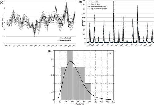
The uncertainty in the seasonal forecast was quantified by generating 10 equiprobable values of JAS precipitation, disaggregating them, and then feeding them into the SWAT model, as described in Section 2.7. The cloud of generated rainfall values is plotted along with the observed precipitation and the best forecast in Fig. 9(a). It shows that the observed rainfall falls within the cloud except for one time. Therefore, a water resource management policy that would ensure that no damage occurs no matter which one of the 10 plausible rainfall amounts occurs would make the area resilient to climate variability. A similar conclusion can be drawn about streamflow (Fig. 9(b)). Finally, for the coming year, a histogram of the possible values of peak precipitation and/or streamflow could be drawn along with an exceedence probability associated with each magnitude. An example of such a histogram (derived from the possible values of the peaks) is presented in Fig. 9(c). Increasing the number of plausible rainfall amounts above 10 would lead to an even smoother histogram and a more precise estimate of the exceedence probability of a given peak flow.

Figure 9. Representation of forecasted rainfall and streamflow uncertainties: (a) rainfall uncertainty, (b) streamflow uncertainty, (c) example of approximated probability distribution function of annual maximum flows. The bars represent a scaled histogram; the line is a gamma fit of peak flows.

The fact that streamflow at the GarbeKorou station in Niger can be forecasted 12 months in advance is of the greatest importance for local policymakers. The methodology presented in this paper can easily be included in a probabilistic cost-benefit analysis of water resource management policies. Furthermore, there is a good chance that even better forecasts can be issued if additional potential predictors such as pressures, wind speeds and directions are investigated using similar techniques. Another possible improvement in the method is to use nonlinear relationships, as the linear model may be too restrictive for describing the relationship between precipitation and SST.

4 Discussion

The statistical models proposed in this study allowed the generation of relatively skillful forecasts of the JAS total rainfall in the Sirba watershed. The performance of our optimal rainfall forecasting model, Method 2 with Pacific Ocean SST (R = 0.677; R² = 0.458) compares favourably to that of the seasonal forecasting models presented in Barnston et al. (1996), Garric et al. (2002), Mo and Thiaw (2002), Barnston et al. (1996) used canonical correlation analysis with quasi-global SST as predictors to forecast rainfall in the African continent. Seasonal rainfall forecasting in the Sahel region obtained a correlation coefficient of 0.33 at 1-month lead time. Garric et al. (2002) used the Atlantic and Indian ocean SST and the Niño-3 index over the April–June period as predictors to forecast the monsoon rainfall (JAS) over central Sahel. A simple regression was tested for each individual predictor. The best correlation coefficients were 0.34–0.53 (R² = 0.12–0.29) at various lead times using the Niño-3 index. Mo and Thiaw (2002) performed an ensemble canonical correlation prediction method to forecast JAS seasonal mean rainfall over the Sahel. The March–May mean global SST was one of various predictors which were used. The simulation skill at each grid point’s rainfall correlation resulted in a mean anomaly correlation of 0.34 (R² = 0.10). Folland et al. (1991) attempted to forecast rainfall in the Sahel using SST as predictor and obtained a correlation coefficient of 0.72 (R² = 0.52) at 1-month lead time. The scores are limited by both the nature of the statistical models used and the inherent unpredictability of weather beyond a certain horizon. Further research on seasonal forecasting models (type of relationships, nature of predictors, etc.) can help improve the performance up to a certain point. Because of limited resources, this paper has only used one type of predictor (SST) and a relatively simple relationship between the predictor and the predictand. It did not consider the possibility of simultaneously using several SST averaging periods to generate a larger predictor vector. There is, therefore, a potential for finding even better rainfall and seasonal forecasting models by testing other types of predictors (pressure, humidity, wind, etc.), by considering nonlinear models and/or combining SST averaging periods. Another potential research direction is the estimation of the economic value of the forecast by looking at the opportunities for economic benefits and the value at risk of flood damage.

Models for which PCA was used to reduce the SST dimensions clearly performed better than those for which CCA was used. While it is difficult to explain with certainty why this happened, the fact that CCA provides a one-column predictor while PCA produces several potential predictors (the PCs) certainly plays a role. Therefore, using PCA increases the chance that one of the retained predictors has a significant link with the predictand. In addition, the results indicate that arbitrarily choosing a single month or a trimester as the SST averaging period may not lead to an optimal JAS rainfall forecasting performance.

To the knowledge of the authors, this paper is the first to combine statistical seasonal forecasting models with rainfall–runoff modelling in the Sahel region. It improves considerably over the categorical forecasts provided by the PRESAO meetings because its results are quantitative and can be readily used in a water management model. The probabilistic hydrographs may, for example, be supplied to a model that would simultaneously estimate irrigation benefits and flood damage and provide the probability of net benefits (or losses) for each sector of the economy. If the probability of loss is significant, policymakers may want to divert some resources in advance to mitigation procedures, or at least be prepared for a significant emergency intervention.

5 Conclusions

This study shows that it is possible to develop skillful statistical rainfall and hydrological seasonal forecasting models with 12-month lag times for the Sirba watershed located in West Africa. Gridded datasets of the Atlantic and Pacific oceans were used as predictors, and the relationship between annual rainfall and SSTs was assumed to be linear. A two-step screening technique was applied where particular grid points were first selected using the coefficient of determination (R²) or the Nash-Sutcliffe coefficient (E_f) of the relationship between the SST at a particular point and the Sirba rainfall, and then principal component analysis (PCA) or canonical correlation analysis (CCA) followed by stepwise regression were used to reduce the dimensions of the predictor vector further to reach a practical size. The results revealed that the model developed using E_f, PCA and stepwise (Method 2) with Pacific Ocean SST was the best for estimating the July–September precipitation in the watershed. At a lag time of 12 months, it forecasted the annual precipitation in the Sirba with moderate skill. The rainfall forecast using the best method was temporally disaggregated and used to force a SWAT model of the watershed. Streamflow at the outlet of the watershed could be forecasted 12 months in advance (R² = 0.552, E_f = 0.487, H = 73.28%). Finally, a simple framework was developed to include uncertainty in the forecasts, paving the road for cost-benefit analysis of management decisions.

Additional information

Funding

The authors thank the International Development Research Centre (Canada) and the National Science and Engineering Research Council of Canada for funding this research.

References

- Abbaspour, K.C., 2012. SWAT-CUP 2012: SWAT calibration and uncertainty programs. Eawag: Swiss Federal Institute of Aquatic Science and Technology. Available from: http://www.neprashtechnology.ca/Downloads/SwatCup/Manual/Usermanual_Swat_Cup.pdf [Accessed 11 March 2014].
- Barnston, A.G., Thiao, W., and Kumar, V., 1996. Long-lead forecasts of seasonal precipitation in Africa using CCA. Weather and Forecasting, 11, 506–520. doi:10.1175/1520-0434(1996)011<0506:LLFOSP>2.0.CO;2
- Biasutti, M., et al., 2008. SST forcings and Sahel rainfall variability in simulations of the twentieth and twenty-first centuries. Journal of Climate, 21, 3471–3486. doi:10.1175/2007JCLI1896.1
- Bossa, A.Y., et al., 2012. Analyzing the effects of different soil databases on modeling of hydrological processes and sediment yield in Benin (West Africa). Geoderma, 173–174, 61–74. doi:10.1016/j.geoderma.2012.01.012
- Brooks, N., 2004. Drought in the African Sahel: long term perspectives and future prospects. Saharan Studies Programme and Tyndall Centre for Climate Change Research, University of East Anglia, UK.
- Busuioc, A., Tomozeiu, R., and Cacciamani, C., 2008. Statistical downscaling model based on canonical correlation analysis for winter extreme precipitation events in the Emilia-Romagna region. International Journal of Climatology, 28, 449–464. doi:10.1002/joc.1547
- Charles, S.P., et al., 2004. Statistical downscaling of daily precipitation from observed and modelled atmospheric fields. Hydrological Processes, 18, 1373–1394. doi:10.1002/hyp.1418
- Chow, V., Maidment, D., and Mays, L., 1988. Applied hydrology. New York: McGraw-Hill Science.
- Christensen, J.H., et al., 2007. Regional climate projections. In: S. Solomon, et al., eds. Climate change 2007: the physical science basis. Contribution of Working Group I to the Fourth Assessment Report of the Intergovernmental Panel on Climate Change. New York: Cambridge University Press, 847–940. SM.11-1-SM–11-46.
- Cibin, R., Sudheer, K.P., and Chaubey, I., 2010. Sensitivity and identifiability of stream flow generation parameters of the SWAT model. Hydrological Processes, 24, 1133–1148. doi:10.1002/hyp.7568
- Dai, A., et al., 2004. The recent Sahel drought is real. International Journal of Climatology, 24, 1323–1331. doi:10.1002/joc.1083
- Demirel, M.C., Venancio, A., and Kahya, E., 2009. Flow forecast by SWAT model and ANN in Pracana basin, Portugal. Advances in Engineering Software, 40, 467–473. doi:10.1016/j.advengsoft.2008.08.002
- Folland, C., et al., 1991. Prediction of seasonal rainfall in the Sahel region using empirical and dynamical methods. Journal of Forecasting, 10, 21–56. doi:10.1002/for.3980100104
- Garric, G., Douville, H., and Déqué, M., 2002. Prospects for improved seasonal predictions of monsoon precipitation over Sahel. International Journal of Climatology, 22, 331–345. doi:10.1002/joc.736
- Hansen, J.W., et al., 2009. Potential value of GCM-based seasonal rainfall forecasts for maize management in semi-arid Kenya. Agricultural Systems, 101, 80–90. doi:10.1016/j.agsy.2009.03.005
- Harms, A.A. and Campbell, T.H., 1967. An extension to the Thomas-Fiering model for the sequential generation of streamflow. Water Resources Research, 3, 653–661. doi:10.1029/WR003i003p00653
- Hayes, M., et al., 2005. Drought monitoring: new tools for the 21st century. In: D.A. White, eds. Drought and water crises: science, technology, and management issues. Boca Raton, LA: Taylor & Francis, 53–69.
- Huang, G., Liu, Y., and Huang, R.H., 2011. The interannual variability of summer rainfall in the arid and semiarid regions of Northern China and its association with the northern hemisphere circumglobal teleconnection. Advances in Atmospheric Sciences, 28, 257–268. doi:10.1007/s00376-010-9225-x
- Huang, Z., Xue, B., and Pang, Y., 2009. Simulation on stream flow and nutrient loadings in Gucheng Lake, Low Yangtze River Basin, based on SWAT model. Quaternary International, 208, 109–115. doi:10.1016/j.quaint.2008.12.018
- Hunt, B.G., 2000. Natural climatic variability and Sahelian rainfall trends. Global and Planetary Change, 24, 107–131. doi:10.1016/S0921-8181(99)00064-8
- IRIN, 2012. West Africa: after the drought, floods-and harvest worries [online]. IRIN News, 14 September 2012. Available from http://www.irinnews.org/report/96313 [Accessed 23 September 2013].
- Jajarmizadeh, M., Harun, S., and Salarpour, M., 2013. An assessment on base and peak flows using a physically-based model. Research Journal of Environmental and Earth Sciences, 5, 49–57.
- Janicot, S., Trzaska, S., and Poccard, I., 2001. Summer Sahel-ENSO teleconnection and decadal time scale SST variations. Climate Dynamics, 18, 303–320. doi:10.1007/s003820100172
- Konte, O., 2011. Vérification des prévisions climatiques saisonnières sur les précipitations en Afrique de l’Ouest (PRESAO) sur la période Juillet-Août-Septembre (JAS) de 1998–2010, au Sénégal. Available from: http://www.academia.edu/3784013/evaluation_of_the_seasonal_forecast_of_rainfall [Accessed 4 October 2013].
- Landman, W.A., et al., 2001. Statistical downscaling of GCM simulations to streamflow. Journal of Hydrology, 252, 221–236. doi:10.1016/S0022-1694(01)00457-7
- Lopez-Bustins, J.A., Martin-Vide, J., and Sanchez-Lorenzo, A., 2008. Iberia winter rainfall trends based upon changes in teleconnection and circulation patterns. Global and Planetary Change, 63, 171–176. doi:10.1016/j.gloplacha.2007.09.002
- Lu, J. and Delworth, T.L., 2005. Oceanic forcing of the late 20th century Sahel drought. Geophysical Research Letters, 32, 1–5. doi:10.1029/2005GL023316
- Marengo, J.A., et al., 2003. Assessment of regional seasonal rainfall predictability using the CPTEC/COLA atmospheric GCM. Climate Dynamics, 21, 459–475. doi:10.1007/s00382-003-0346-0
- Masih, I., et al., 2011. Assessing the impact of areal precipitation input on streamflow simulations using the SWAT model. JAWRA Journal of the American Water Resources Association, 47, 179–195. doi:10.1111/j.1752-1688.2010.00502.x
- Misra, V., 2003. The influence of Pacific SST variability on the precipitation over Southern Africa. Journal of Climate, 16, 2408–2418. doi:10.1175/2785.1
- Mo, K.C. and Thiaw, W.M., 2002. Ensemble canonical correlation prediction of precipitation over the Sahel. Geophysical Research Letters, 29, 11–1–11–4. doi:10.1029/2002GL015075
- Neitsch, S.L., et al., 2009. Soil and Water Assessment Tool theoretical document version 2009 [online]. USA: Texas A&M University. Texas Water Resources Institute Technical Report no. 406. Available from: http://twri.tamu.edu/reports/2011/tr406.pdf [Accessed 14 March 2014]
- Oubeidillah, A.A., Tootle, G., and Anderson, S.-R., 2012. Atlantic Ocean sea-surface temperatures and regional streamflow variability in the Adour-Garonne basin, France. Hydrological Sciences Journal, 57 (3), 496–506. doi:10.1080/02626667.2012.659250
- Palmer, T.N., 1986. Influence of the Atlantic, Pacific and Indian Oceans on Sahel rainfall. Nature, 322, 251–253. doi:10.1038/322251a0
- Raje, D. and Mujumdar, P.P., 2011. A comparison of three methods for downscaling daily precipitation in the Punjab region. Hydrological Processes, 25, 3575–3589. doi:10.1002/hyp.8083
- Samimi, C., Fink, A.H., and Paeth, H., 2012. The 2007 flood in the Sahel: causes, characteristics and its presentation in the media and FEWS NET. Natural Hazards and Earth System Science, 12, 313–325. doi:10.5194/nhess-12-313-2012
- Schepen, A., Wang, Q.J., and Robertson, D.E., 2012. Combining the strengths of statistical and dynamical modeling approaches for forecasting Australian seasonal rainfall. Journal of Geophysical Research: Atmospheres, 117, 148–227. doi:10.1029/2012JD018011
- Schuol, J. and Abbaspour, K.C., 2007. Using monthly weather statistics to generate daily data in a SWAT model application to West Africa. Ecological Modelling, 201, 301–311. doi:10.1016/j.ecolmodel.2006.09.028
- Sood, A., Muthuwatta, L., and McCartney, M., 2013. A SWAT evaluation of the effect of climate change on the hydrology of the Volta River basin. Water International, 38, 297–311. doi:10.1080/02508060.2013.792404
- Trambauer, P., et al., 2013. A review of continent scale hydrological models and their suitability for drought forecasting in (sub-Saharan) Africa. Physics and Chemistry of the Earth, 66, 16–26.
- Tripathi, M.P., et al., 2004. Hydrological modelling of a small watershed using generated rainfall in the soil and water assessment tool model. Hydrological Processes, 18, 1811–1821. doi:10.1002/hyp.1448
- Wang, G., et al., 2014. Using the SWAT model to assess impacts of land use changes on runoff generation in headwaters. Hydrological Processes, 28, 1032–1042. doi:10.1002/hyp.9645
- Wetterhall, F., Halldin, S., and Xu, C., 2005. Statistical precipitation downscaling in central Sweden with the analogue method. Journal of Hydrology, 306, 174–190. doi:10.1016/j.jhydrol.2004.09.008
- Wilby, R.L. and Wigley, T.M.L., 1997. Downscaling general circulation model output: a review of methods and limitations. Progress in Physical Geography, 21, 530–548. doi:10.1177/030913339702100403
- Xu, C.-Y., 1999. Climate change and hydrologic models: a review of existing gaps and recent research developments. Water Resources Management, 13, 369–382. doi:10.1023/A:1008190900459
- Xu, Z.X., et al., 2009. Assessment of runoff and sediment yield in the Miyun Reservoir catchment by using SWAT model. Hydrological Processes, 23, 3619–3630. doi:10.1002/hyp.7475