Predicting daily pan evaporation by soft computing models with limited climatic data

Abstract

Accurate prediction of daily pan evaporation (PE) is important for monitoring, surveying, and management of water resources as well as reservoir management and evaluation of drinking water supply systems. This study develops and applies soft computing models to predict daily PE in a dry climate region of south-western Iran. Three soft computing models, namely the multilayer perceptron-neural networks model (MLP-NNM), Kohonen self-organizing feature maps-neural networks model (KSOFM-NNM), and gene expression programming (GEP), were considered. Daily PE was predicted at two stations using temperature-based, radiation-based, and sunshine duration-based input combinations. The results obtained by the temperature-based 3 (TEM3) model produced the best results for both stations. The Mann-Whitney U test was employed to compute the rank of different input combination for hypothesis testing. Comparison between the soft computing models and multiple linear regression model (MLRM) demonstrated the superiority of MLP-NNM, KSOFM-NNM, and GEP over MLRM. It was concluded that the soft computing models can be successfully employed for predicting daily PE in south western Iran.

Editor D. Koutsoyiannis

Résumé

La prévision précise de l’évaporation journalière au bac (EJB) est importante pour la mesure, le contrôle et la gestion des ressources en eau ainsi que pour la gestion des réservoirs et l’évaluation des systèmes d’alimentation en eau potable. Cette étude développe et applique des modèles flous pour prévoir l’EJB dans une région de climat sec du Sud-Ouest de l’Iran. Trois modèles flous ont été considérés : un réseau de neurones perceptron multicouche (RNPM), un réseau de neurones auto-organisé de Kohonen (RNAOK) et la programmation d’expression génétique (PEG). L’EJB a été prévue pour deux stations, en utilisant des combinaisons d’entrées issues de la température, du rayonnement et de la durée d’ensoleillement. Les meilleurs résultats pour les deux stations ont été obtenus par le modèle 3 basé sur la température (TEM3). Le test U de Mann-Whitney a été utilisé pour calculer le classement de différentes combinaisons d’entrées afin de tester les hypothèses. La comparaison entre les modèles flous et un modèle de régression linéaire multiple (MRLM) a démontré la supériorité de RNPM, RNAOK et PEG sur MRLM. On en conclut que les modèles flous peuvent être utilisés avec succès pour prévoir l’EJB dans le Sud-Ouest de l’Iran.

Key words:

• soft computing models
• pan evaporation
• Mann-Whitney U test
• limited climatic data
• multiple linear regression

Mots clefs:

• modèles flous
• évaporation au bac
• test U de Mann-Whitney
• données climatiques limitées
• régression linéaire multiple

INTRODUCTION

Evaporation is the process of conversion of liquid water to water vapor. Evaporation from a free water surface depends on energy supply, the difference in vapor pressure between the surface and atmosphere, and exchange of surface air with the surrounding atmospheric air (Penman 1948). Evaporation from the land surface consumes about 61 percent of total global precipitation (Chow et al. 1988), and hence it is an important component of the hydrological cycle and its quantitative study is one of the important issues in water resources engineering. Nevertheless, the continuous hydrological simulation models often need at least the input data of precipitation and evaporation (Kay and Davies 2008). Pan evaporation (PE) is widely used to estimate evaporation from lakes and reservoirs (Finch 2001).

Both direct and indirect methods have been employed to estimate evaporation. Direct methods, such as evaporation pans, have also been used and compared to estimate evaporation by other methods (Choudhury 1999, Vallet-Coulomb et al. 2001). The most widely used pan is the U.S. Weather Bureau Class A pan, which is 21 cm in diameter, 25.5 cm deep, and mounted on a timber grid 15 cm above the soil surface. The pan coefficient is a function of the type of pan and the size and state of the upwind buffer zone, and defines the ratio of the amount of evaporation from a large body of water to that measured from an evaporation pan. It ranges from 0.35 to 0.85 for different conditions (Allen et al. 1998). Indirect methods for estimating evaporation are based on different climatic variables, but some of these techniques require data which cannot be easily obtained (Rosenberry et al. 2007).

During the past decade, a variety of soft computing models have been developed and applied for the estimation of evaporation (Bruton et al. 2000, Sudheer et al. 2002, Terzi and Erol Keskin 2005, Keskin and Terzi 2006, Kişi 2006, 2009, Tan et al. 2007, Kim and Kim 2008, Tabari et al. 2010, Chang et al. 2010, 2013, Guven and Kişi 2011, Shiri and Kişi 2011, Shiri et al. 2011, Kim et al. 2012, 2013, Kişi et al. 2012, Shiri et al. 2014). In this study, soft computing models, including the multilayer perceptron-neural networks model (MLP-NNM), Kohonen self-organizing feature maps-neural networks model (KSOFM-NNM), and gene expression programming (GEP), have been applied to predict daily PE from available climatic data.

MLP-NNM is a layered feedforward network model, typically trained with static backpropagation, and has found its way into countless applications requiring static pattern classification (Haykin 2009). Kim et al. (2009) compared MLP-NNM with support vector machines neural networks model (SVM-NNM), and constructed credible monthly PE data from the disaggregation of yearly PE data.

KSOFM-NNM transforms an input of arbitrary dimension into a one or two dimensional discrete map subject to a topological (neighborhood preserving) constraint. The feature maps are computed using the Kohonen unsupervised learning. The output of SOFM can be used as input to a supervised classification neural network, such as MLP. Chang et al. (2010) proposed a self-organizing map (SOM) neural network to assess the variability of daily evaporation based on meteorological variables. They demonstrated that the topological structures of SOM could yield a meaningful map to present clusters of meteorological variables and the networks could well estimate daily evaporation.

GEP employs a parse tree structure for the search of solutions. This technique has the capability for deriving a set of explicit formulations that rule the phenomenon and describe the relationship between independent and dependent variables using various operators. Shiri and Kişi (2011) investigated the capabilities of GEP to improve the accuracy of daily evaporation estimation and demonstrated that the proposed GEP performed quite well in modeling evaporation from climatic data.

Although there have been many soft computing models, their applications for predicting evaporation have been limited. The present study investigates the capabilities of MLP-NNM, KSOFM-NNM, and GEP, and a conventional multiple linear regression model (MLRM) for predicting daily PE.

MATERIALS AND METHODS

Data used

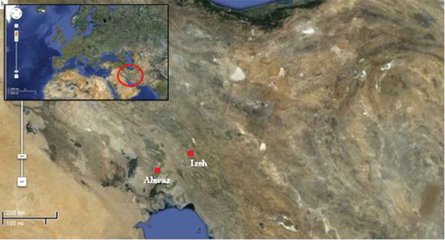
Daily climatic data of two automated weather stations, Ahwaz station (latitude 31°20′N, longitude 48°40′E, elevation 22.5 m a.m.s.l.) and Izeh station (latitude 31°51′N, longitude 49°52′E, elevation 767 m a.m.s.l.), operated by the Khozestan Meteorological Organization (KMO) in Iran, were used in this study. The distance between Ahwaz and Izeh stations is about 205 km. Figure 1 shows the location of weather stations in south-western Iran. The basic data of Ahwaz and Izeh stations consisted of seven years (2002–2008) of daily records of mean air temperature (T), mean wind speed (U), sunshine duration (SD), mean relative humidity (RH), and pan evaporation (PE), as well as computed extraterrestrial radiation (R).

Fig. 1 Location of weather stations in south-western Iran.

The cross-validation method provides a rigorous test of neural networks skill (Dawson and Wilby 2001). It involves dividing the available data into three sets: a training set, a cross-validation set, and a testing set. The training set is used to fit the connection weights of neural network model, the cross-validation set is used to select the model variant that provides the best level of generalization, and the testing set is used to evaluate the chosen model against unseen data. In this case, the first five years of data (71.4% of the whole data set, 2002–2006) were used to train MLP-NNM, KSOFM-NNM, and GEP, and the remaining two years data (2007–2008) were used to cross-validate (14.3% of the whole data set, 2007) and test (14.3% of the whole data set, 2008) MLP-NNM, KSOFM-NNM, and GEP, respectively. The reason for this partition is that one full seasonal cycle was used for training, cross-validation, and testing. This also ensures the statistical properties of training, cross-validation and testing data sets to be of similar order (Jain et al. 2008). Tokar and Johnson (1999) suggested that the data length has less effect than the data quality on the performance of a neural networks model. Sivakumar et al. (2002) suggested that it is imperative to select a good training data from the available data series. They indicated that the best way to achieve a good training performance seems to be to include most of the extreme events, such as very high and very low values, in the training data. Table 1 shows statistical parameters of the data used during the study period. In Table 1, X_mean, X_max, X_min, S_x, C_v, C_sx, SE, 25th percentile, 75th percentile, and 90th percentile denote the mean, maximum, minimum, standard deviation, coefficient of variation, skewness coefficient, standard error, 25th percentile, 75th percentile, and 90th percentile values of each variable, respectively. In both stations, the pan evaporation shows high variation (see C_v values in Table 1), whereas the extraterrestrial radiation has the lowest variation among other weather variables. The mean wind speed and sunshine duration data show high skewed distributions for both stations. Figure 2 shows the time series of daily pan evaporation and temperature values for both stations during the study period.

Fig. 2 Daily pan evaporation and temperature values during the study period (2002–2008).

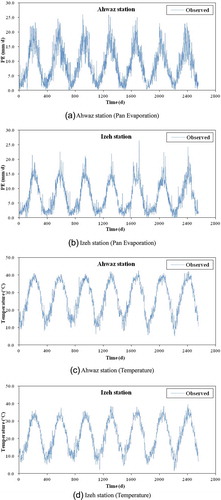
Table 1 Statistical parameters of the data used for the study period (2002–2008).

Station	Data	Unit	Xmean	Xmax	Xmin	Sx	Cv	Csx	SE	25th Percentile	75th Percentile	90th Percentile
Ahwaz	T	°C	26.53	42.50	5.20	9.61	0.36	−0.23	0.19	17.60	35.80	38.20
	U	m/s	5.24	33.00	0.00	2.51	0.48	1.54	0.05	3.00	7.00	8.00
	SD	h	8.69	13.20	0.00	3.48	0.40	−1.18	0.07	7.40	11.20	12.00
	RH	%	41.86	93.50	9.00	19.00	0.45	0.54	0.38	25.00	56.00	69.00
	R	MJ/m^2	19.04	33.76	0.00	6.69	0.35	−0.22	0.13	12.76	25.04	27.31
	PE	mm	8.88	26.00	0.00	5.72	0.64	0.47	0.11	3.80	13.15	17.40
Izeh	T	°C	21.40	39.50	1.50	9.00	0.42	−0.04	0.18	13.20	29.90	33.10
	U	m/s	5.49	30.00	0.00	2.75	0.50	0.83	0.05	4.00	7.00	8.00
	SD	h	8.65	13.50	0.00	3.66	0.42	−1.09	0.07	7.10	11.30	12.30
	RH	%	40.95	96.00	0.00	20.87	0.51	0.38	0.41	22.50	58.50	70.80
	R	MJ/m^2	19.06	31.77	2.34	7.04	0.37	−0.21	0.14	12.64	25.31	27.94
	PE	mm	7.20	26.40	0.01	5.02	0.70	0.56	0.10	2.80	11.71	14.16

Multilayer perceptron-neural networks model (MLP-NNM)

The MLP-NNM has an input layer, an output layer, and one or more hidden layers between the input and output layers. Each of the nodes in a layer is connected to all the nodes of the next layer, and the nodes in one layer are connected only to the nodes of the immediate next layer (Haykin 2009). In this study, MLP-NNM is trained with the QuickProp backpropagation algorithm (BPA) which is a training method that operates much faster in the batch mode than the conventional BPA (NeuroDimension 2005). It has the additional advantage that it is not sensitive to the learning rate and the momentum. Results of the output layer for the temperature-based model (i.e. TEM3) can be written as:

(1)

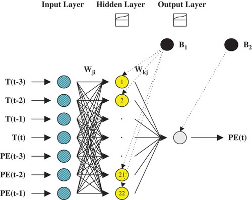
where i,j,k are the input, hidden and the output layers, respectively; PE(t) is the current PE (mm/d) at Ahwaz and Izeh stations; Φ₁(·) is the linear sigmoid transfer function of the hidden layer; Φ₂(·) is the linear sigmoid transfer function of the output layer; W_kj are the connection weights between hidden and output layers; W_ji the connection weights between input and hidden layers; X(t) is the time series data of input nodes comprising seven inputs corresponding to T(t – 3), T(t – 2), T(t – 1), T(t), PE(t – 3), PE(t – 2), PE(t – 1); B₁ is the bias in the hidden layer; and B₂ is the bias in the output layer. Figure 3 shows the structure of MLP-NNM based on TEM3 (7-22-1) developed in this study.

Fig. 3 Structure of MLP-NNM based on TEM 3 (7-22-1).

Kohonen self-organizing feature maps-neural networks model (KSOFM-NNM)

The KSOFM-NNM performs mapping from a continuous input space to a discrete output space, preserving the topological properties of the input nodes (Kohonen 1990, 2001, Principe et al. 2000, Hsu et al. 2002, Lin and Chen 2005, 2006, Chang et al. 2007, Lin and Wu 2007, 2009). KSOFM-NNM consists of four layers, that is, the input layer, the Kohonen layer, the hidden layer, and the output layer. The input layer is composed of n input nodes, each connected to all nodes of the Kohonen layer. The Kohonen layer consists of [n₁ × n₁] matrices. In this study, KSOFM-NNM classifies each input node and determines to which node in the hidden layer it must be routed for predicting daily PE of the output layer.

The mathematical description of KSOFM-NNM is as follows. Let W_ji represent the connection weights between the input and Kohonen layers of KSOFM-NNM. The Euclidean distance between the input and the Kohonen nodes can be written as:

(2)

where i,j are the input and the Kohonen layers, respectively; and d_j is the Euclidean distance between the input and the Kohonen nodes. The distance to each of the Kohonen nodes is computed and the node, c, which has the smallest distance, is selected, i.e. d_c = min(d_j), for all the Kohonen nodes.

The connection weights between the input and the Kohonen layers of KSOFM-NNM are carried out using unsupervised training. The connection weights, W_ji, are initialized to randomly select values for unsupervised training. They are then adjusted so that the nodes which are in the topological neighborhood function Λ_c of node c, which was determined to be closest to the current input node, are moved towards the input node using an iterative adjustment rules. The connection weights can be written as:

(3)

where m is the training iteration; Λ_c is the size of a neighborhood around the winner node c; and η(m) is the step size at the training iteration m. This procedure is applied several times to the whole data of input nodes.

The hidden layer can receive the results calculated from S_j and the connection weights between the Kohonen and hidden layers, which can be written as:

(4)

where k is the hidden layer; W_kj are the connection weights between the Kohonen and hidden layers; S_j is the result calculated from d_j and the Kohonen layer; and U_k is the result calculated from S_j and the connection weights between the Kohonen and hidden layers. The output layer can receive the results calculated from U_k and the connection weights between the hidden and output layers. The results of the output layer based on TEM 3 can be written as:

(5)

where W_lk are the connection weights between hidden and output layers; and the parameters are as defined for equation (1). Figure 4 shows the structure of KSOFM-NNM based on TEM 3 (7‐[5 × 5]‐22‐1) developed in this study.

Fig. 4 Structure of KSOFM-NNM based on TEM 3 (7-[5 × 5]-22-1).

Gene expression programming (GEP)

GEP is a genetic algorithm (GA), as it uses populations of individuals, selects them according to fitness, and genetic variation using one or more genetic operators (Ferreira 2006). One of the strengths of GEP over other soft computing models is its capability to produce explicit formulations (model expression) of the relationship that rules the physical phenomenon. However, there are also some problems regarding a GEP application. For example, in some cases, the program size (depth of parse tree) starts growing which leads to producing a nested function (bloat phenomenon). To overcome this weakness, one should employ some penalization of complex models (limitation of the depth of the parse tree) to produce parsimonious relations.

The procedure to predict daily PE (dependent variable) using the various input combinations (independent variables) is as follows:

• Select a fitness function;

• choose a set of terminals T and a set of functions F to create chromosomes;

• choose the chromosomal architecture;

• choose the linking function;

• choose the genetic operators.

Figure 5 shows equations using mathematical functions and the parse trees. In this study, the GeneXpro program (Ferreira 2001) was applied for predicting daily PE.

Fig. 5 Equations using (a) mathematical functions and (b) the parse trees.

Performance statistics

The performance of the soft computing models was evaluated using four different standard statistical criteria: the coefficient of correlation (CC), the root mean square error (RMSE), the scatter index (SI) (Shiri and Kişi 2011), and the Nash-Sutcliffe efficiency (NS) (Nash and Sutcliffe 1970, ASCE 1993). CC, a measure of the accuracy between predicted and observed PE, is generally used for comparisons of alternative models. According to Legates and McCabe (1999), the correlation coefficient (CC) alone should not be used to evaluate the goodness-of-fit of model simulations, since the standardization inherent in CC as well as its sensitivity to outliers yields high CC values even when the model performance may not be good. Therefore, additional statistical measures (e.g. RMSE and NS) should be applied to evaluate the model performance. RMSE is a measure of the residual variance and can be defined as the square root of the average value of the squares of the differences between predicted and observed PE values. SI is the dimensionless RMSE and is expressed as a percentage mean of observed PE. NS, a dimensionless measure, is the coefficient of efficiency and can be used to indicate the relative assessment of the model performance (Nash and Sutcliffe 1970). The NS efficiency is one of the most widely used criteria for calibration and evaluation of hydrological models with the observed data (Gupta et al. 2009). Table 2 shows mathematical expressions of the statistical criteria.

Table 2 Mathematical expressions of the statistical criteria.

Statistical Index	Equation
CC
RMSE
SI
NS

y_i(x): observed PE (mm/d); : predicted PE (mm/d); u_y: mean of the observed PE (mm/d); : mean of the predicted PE (mm/d); and n: total number of daily PE considered.

RESULTS AND DISCUSSION

Selection of input nodes and data normalization

The input nodes for soft computing models were selected, based on the serial correlation of daily PE and the cross-correlation between (a) daily PE and T (temperature-based), (b) daily PE and R (radiation-based), and (c) daily PE and SD (sunshine duration-based). The serial correlation of daily PE was calculated to select the optimal input nodes of soft computing models. The maximum lag-time of cross-correlations between (i) daily PE and T, (ii) daily PE and R, and (iii) daily PE and SD were calculated. Figure 6(a) and (b) shows serial correlations and cross-correlations for both stations. Each input combination was selected, based on the lag-time for T, R, and SD corresponding to the lag-time of PE, and the current daily PE was chosen as the only output node for the soft computing models. Table 3 shows the input combinations in this study.

Fig. 6 Serial correlations and cross-correlations.

Table 3 Input combinations of MLP-NNM, KSOFM-NNM, and GEP.

Classification	Expression	Input combination
Temperature-based	TEM 1	T(t – 1), T(t), PE(t – 1)
	TEM 2	T(t – 2), T(t – 1), T(t), PE(t – 2), PE(t – 1)
	TEM 3	T(t – 3), T(t – 2), T(t – 1), T(t), PE(t – 3), PE(t – 2), PE(t – 1)
Radiation-based	RAD 1	R(t – 1), R(t), PE(t – 1)
	RAD 2	R(t – 2), R(t – 1), R(t), PE(t – 2), PE(t – 1)
	RAD 3	R(t – 3), R(t – 2), R(t – 1), R(t), PE(t – 3), PE(t – 2), PE(t – 1)
Sunshine duration-based	SUN 1	SD(t – 1), SD(t), PE(t – 1)
	SUN 2	SD(t – 2), SD(t – 1), SD(t), PE(t – 2), PE(t – 1)
	SUN 3	SD(t – 3), SD(t – 2), SD(t – 1), SD(t), PE(t – 3), PE(t – 2), PE(t – 1)

Data for input and output nodes were normalized for preventing and overcoming problems associated with extreme values. An important reason for the normalization of input and output nodes is that each of those nodes represents an observed value in a different unit. Such input and output nodes are normalized, and the input and output nodes in dimensionless units are expressed. The similarity effect of input and output nodes is thus eliminated (Sudheer et al. 2002, 2003). For data normalization, the climatic data for input and output nodes were scaled to the range of [0 1] as:

(6)

where for the specific node Y_norm is the normalized dimensionless data; Y_i is the observed data; Y_min is the minimum data; and Y_max is the maximum data.

Performance of MLP-NNM

Cross-validation performance was used to overcome the overfitting problem for MLP-NNM, KSOFM-NNM and GEP using cross-validation data. In the literature, this method has often been applied for training (Haykin 2009). After training and cross-validation of soft computing models, MLP-NNM, KSOFM-NNM, and GEP were tested by determining whether or not the model meets the objectives of modelling within some pre-established criteria.

Table 4 shows the final structure of MLP-NNM, indicating the number of nodes of each MLP-NNM in input, hidden, and output layers, respectively. A difficult task with soft computing models is to choose the number of hidden layers and nodes. The network geometry is problem dependent (Kişi 2007). This study adopted one hidden layer for the construction of MLP-NNM and KSOFM-NNM, since it is well known that one hidden layer is enough to represent the nonlinear complex relationship (Kumar et al. 2002). Table 4 also shows the test statistics of each MLP-NNM in terms of CC, RMSE, SI, and NS for both stations. From Table 4, it can be observed that TEM3 produced the best results among other input combinations for both stations. Table 4 also reveals that increasing the lag-time intervals from 1 day to 3 days for temperature-based, radiation-based, and sunshine duration-based input combinations increases the model accuracy to some extent. Figure 7(a)–(f) compares observed and predicted PE values for the optimal MLP-NNM during the test period for both stations. The superiority of TEM3 over RAD3 and SUN3 is clearly seen from Fig. 7(a)–(f).

Fig. 7 Comparison of observed and predicted PE values for the optimal MLP-NNM (testing data).

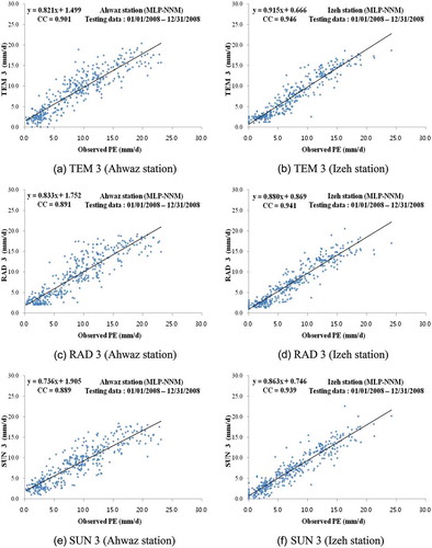
Table 4 Statistics results of the performance of MLP-NNM (testing data).

Station	Input combination	Structure	Statistical criteria
			CC	RMSE (mm)	SI	NS
Ahwaz	TEM1	3-45-1	0.889	2.541	0.291	0.791
	TEM2	5-30-1	0.893	2.501	0.286	0.797
	TEM3	7-22-1	0.901	2.417	0.277	0.811
	RAD1	3-45-1	0.883	2.655	0.304	0.772
	RAD2	5-30-1	0.887	2.576	0.295	0.785
	RAD3	7-22-1	0.891	2.549	0.292	0.790
	SUN1	3-45-1	0.878	2.685	0.308	0.767
	SUN2	5-30-1	0.881	2.667	0.305	0.770
	SUN3	7-22-1	0.889	2.596	0.297	0.781
Izeh	TEM1	3-45-1	0.942	1.712	0.231	0.887
	TEM2	5-30-1	0.943	1.710	0.231	0.887
	TEM3	7-22-1	0.946	1.646	0.222	0.895
	RAD1	3-45-1	0.936	1.793	0.242	0.876
	RAD2	5-30-1	0.940	1.739	0.235	0.883
	RAD3	7-22-1	0.941	1.720	0.232	0.886
	SUN1	3-45-1	0.930	1.905	0.257	0.856
	SUN2	5-30-1	0.936	1.803	0.243	0.874
	SUN3	7-22-1	0.939	1.778	0.240	0.878

Performance of KSOFM-NNM

The general structure of KSOFM-NNM includes the input layer, Kohonen layer, hidden layer, and output layer. Determining the appropriate size of matrices in the Kohonen layer is important for model efficiency. Since there is no standard method for finding the optimal number of matrices in the Kohonen layer, the optimal matrices size in the Kohonen layer was based on the trial and error method. In this study, the Kohonen layer consisted of [5 × 5] matrices with the minimum RMSE of all the input combinations using the trial and error method among the various matrices, including [4 × 4, 5 × 5, 6 × 6, and 7 × 7]. Chang et al. (2010) determined the optimal size SOM networks with [6 × 6] matrices using the trial and error method among the various matrices, such as [3 × 3, 4 × 4, 5 × 5, 6 × 6, 7 × 7, and 8 × 8].

Table 5 represents the final structure of KSOFM-NNM and indicates the number of nodes of each KSOFM-NNM in input, Kohonen, hidden, and output layers, respectively. Table 5 also shows the test statistics of each KSOFM-NNM in terms of CC, RMSE, SI, and NS for both stations. From Table 5, it can be observed that TEM3 produced the best results among other input combinations for both stations. Table 5 also reveals that increasing the lag-time intervals from 1 day to 3 days for temperature-based, radiation-based, and sunshine duration-based input combinations increases the model accuracy to some extent. Figure 8(a)–(f) compares observed and predicted PE values for the optimal KSOFM-NNM during the test period for both stations. As found for MLP-NNM, the better accuracy of TEM3 can be clearly seen from Fig. 8(a)–(f) for both stations.

Fig. 8 Comparison of observed and predicted PE values for the optimal KSOFM-NNM (testing data).

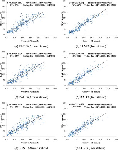
Table 5 Statistical results of the performance of KSOFM-NNM (testing data).

Station	Input combination	Structure	Statistical criteria
			CC	RMSE (mm)	SI	NS
Ahwaz	TEM1	3-[5X5]-45-1	0.895	2.487	0.285	0.800
	TEM2	5-[5X5]-30-1	0.903	2.386	0.273	0.816
	TEM3	7-[5X5]-22-1	0.904	2.380	0.273	0.816
	RAD1	3-[5X5]-35-1	0.895	2.504	0.287	0.797
	RAD2	5-[5X5]-30-1	0.896	2.480	0.284	0.800
	RAD3	7-[5X5]-22-1	0.899	2.457	0.281	0.804
	SUN1	3-[5X5]-45-1	0.882	2.644	0.303	0.774
	SUN2	5-[5X5]-30-1	0.889	2.549	0.292	0.790
	SUN3	7-[5X5]-22-1	0.894	2.513	0.288	0.796
Izeh	TEM1	3-[5X5]-45-1	0.937	1.790	0.242	0.876
	TEM2	5-[5X5]-30-1	0.942	1.715	0.231	0.886
	TEM3	7-[5X5]-22-1	0.951	1.590	0.215	0.902
	RAD1	3-[5X5]-45-1	0.927	1.921	0.259	0.857
	RAD2	5-[5X5]-30-1	0.932	1.848	0.249	0.868
	RAD3	7-[5X5]-22-1	0.943	1.696	0.229	0.889
	SUN1	3-[5X5]-45-1	0.915	2.149	0.290	0.822
	SUN2	5-[5X5]-30-1	0.931	1.871	0.252	0.865
	SUN3	7-[5X5]-22-1	0.940	1.772	0.239	0.879

Performance of GEP

The various forms of GEP were developed using the same input combinations as for MLP-NNM and KSOFM-NNM. A step-by-step procedure of GEP predicting daily PE is as follows: The first step was the selection of the appropriate fitness function which may take various shapes. For mathematical applications, one usually applies small relative or absolute errors to discover a good and applicable solution (Ferreira 2001). According to the MLP-NNM and KSOFM-NNM, the optimal input combination (TEM3) was used with the default function set of GeneXpro for the selection of one of the fitness functions.

The second step consisted of choosing the set of terminals and the set of functions to create chromosomes. In the current problem, the terminal set included the various input combinations. The study examined the various combinations of these parameters as input variables for GEP to evaluate the degree of effect of each of these variables on the daily PE values at designated time steps. A set of preliminary model runs was carried out to test the performances of models with these function sets and one was selected to use in the next stage of study. All of these procedures were performed for GEP based on TEM3 by using the RRSE fitness function and addition linking function. Table 6 shows the preliminary selection of basic functions and linking functions using the SI index for both stations. From comparison of various GEP operators listed in Table 6, it can be concluded that the F5 function set surpassed all of the other four structures.

Table 6 Preliminary selection of basic functions and linking functions using SI index.

	Definition	SI
		Ahwaz	Izeh
F1	{+, - , × ,÷}	0.36	030
F2	{ +, - , × ,÷, ln,e^x}	0.40	0.32
F3	{ +, - , × ,÷, ^3√,√,x^2,x^3}	0.34	0.28
F4	{ +, - , × ,÷, ln,e^x,^3√,√, x^2,x^3}	0.31	0.28
F5	{ +, - , × ,÷, ln,e^x,^3√,√, x^2,x^3, sin x, cos x, arctgx}	0.28	0.23
Linking function
Addition		0.28	0.23
Multiplication		0.30	0.26
Subtraction		0.30	0.30
Division		0.32	0.33

The third step was to choose the chromosomal architecture. The length of head, h = 8, and three genes per chromosomes were employed, which are the commonly used values in the literature (Ferreira 2001). The fourth step was to choose the linking function, which should be chosen as ‘addition’ or ‘multiplication’ for algebraic sub-trees (Ferreira 2001). It can be also concluded from Table 6 that addition linking function surpasses all of the other three linking functions. The final step was to choose the genetic operators.

Table 7 shows the test statistics of each GEP in terms of CC, RMSE, SI, and NS for both stations. From Table 7, it can be observed that TEM3 produced the best results among other input combinations for both stations. Table 7 also reveals that increasing the lag-time intervals from 1 day to 3 days for temperature-based, radiation-based, and sunshine duration-based input combinations increased the model accuracy to some extent. Figure 9(a)–(f) compares observed and predicted PE values for the optimal GEP during the test period for both stations. From the fit line equations and CC values given in Fig. 9(a)–(f), it is clear that TEM3 performed better than did RAD3 and SUN3. Comparison of Tables 4, 5, and 7 revealed that KSOFM-NNM slightly outperformed MLP-NNM and GEP, but differences between the results of the three approaches were not significant and all three of them may be considered as alternative tools for predicting daily PE. Figure 10(a)–(f) shows observed and predicted PE values of MLP-NNM, KSOFM-NNM, and GEP for optimal input combination (TEM3) during the test period for both stations.

Fig. 9 Comparison of observed and predicted PE values for the optimal GEP (testing data).

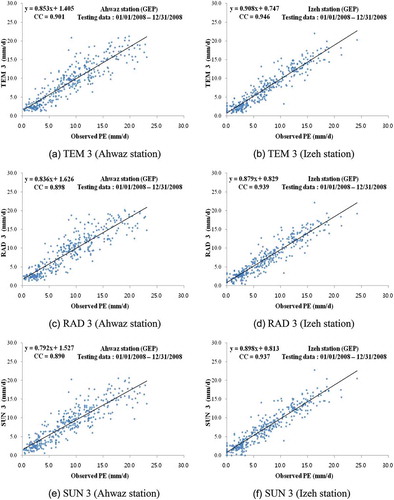
Fig. 10 Observed and predicted PE values for the optimal input combination (TEM 3, 2002–2008).

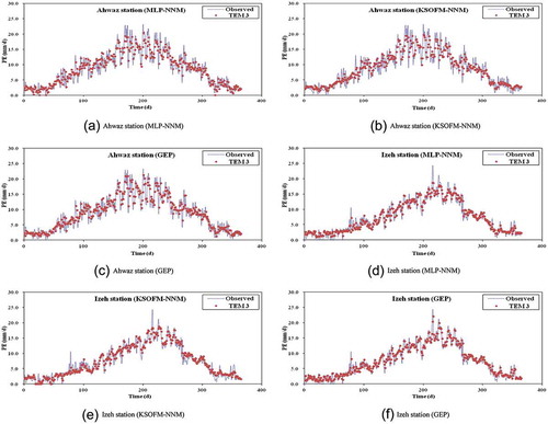
Table 7 Statistical results of the performance of GEP (testing data).

Station	Input combination	Statistical criteria
		CC	RMSE (mm)	SI	NS
Ahwaz	TEM 1	0.894	2.494	0.283	0.799
	TEM 2	0.900	2.431	0.279	0.809
	TEM 3	0.901	2.429	0.278	0.809
	RAD 1	0.892	2.517	0.288	0.795
	RAD 2	0.896	2.474	0.283	0.802
	RAD 3	0.898	2.456	0.281	0.805
	SUN 1	0.876	2.698	0.309	0.764
	SUN 2	0.884	2.616	0.300	0.778
	SUN 3	0.890	2.542	0.291	0.791
Izeh	TEM 1	0.941	1.718	0.232	0.886
	TEM 2	0.943	1.701	0.230	0.888
	TEM 3	0.946	1.657	0.224	0.894
	RAD 1	0.937	1.775	0.240	0.878
	RAD 2	0.938	1.756	0.237	0.881
	RAD 3	0.939	1.747	0.236	0.882
	SUN 1	0.930	1.902	0.257	1.364
	SUN 2	0.935	1.817	0.245	1.312
	SUN 3	0.937	1.778	0.240	1.302

The Mann-Whitney U test, one of the tests for homogeneity analyses, was performed to compare observed and predicted PE values to evaluate the confidence level of soft computing models. It is a nonparametric alternative to the two-sample t test for two independent samples and can be used to test whether two independent samples have been taken from the same population (McCuen 1993, Kottegoda and Rosso 1997, Ayyub and McCuen 2003, Singh et al. 2007). The critical value of the z statistic was computed for the level of significance. If the computed value of z is greater than the critical value of z, the null hypothesis—that the two independent samples are from the same population—should be rejected and the alternative hypothesis should be accepted.

Table 8 shows the results of the Mann-Whitney U test between observed and predicted PE values for the test data of soft computing models, including TEM3, RAD3, and SUN3. The critical value of z statistic was computed as z_0.05 = 1.960 for the 5% level of significance. Since the computed values of z for both stations were not significant, the null hypothesis—that the two independent samples are from the same population—was accepted for the soft computing models of both stations.

Table 8 Results of the Mann-Whitney U test.

Station	Model	Input combination	Level of significance	Mann-Whitney U test
				Critical z statistic	Computed z statistic	Null hypothesis
Ahwaz	MLP-NNM	TEM3	0.05	1.960	–0.381	Accept
		RAD3	0.05	1.960	–0.311	Accept
		SUN3	0.05	1.960	–0.205	Accept
	KSOFM-NNM	TEM3	0.05	1.960	–0.251	Accept
		RAD3	0.05	1.960	–0.768	Accept
		SUN3	0.05	1.960	–0.162	Accept
	GEP	TEM3	0.05	1.960	–0.235	Accept
		RAD3	0.05	1.960	–0.117	Accept
		SUN3	0.05	1.960	–0.432	Accept
Izeh	MLP-NNM	TEM3	0.05	1.960	–0.516	Accept
		RAD3	0.05	1.960	–0.182	Accept
		SUN3	0.05	1.960	–0.708	Accept
	KSOFM-NNM	TEM3	0.05	1.960	–0.356	Accept
		RAD3	0.05	1.960	–1.463	Accept
		SUN3	0.05	1.960	–0.790	Accept
	GEP	TEM3	0.05	1.960	–0.080	Accept
		RAD3	0.05	1.960	–0.125	Accept
		SUN3	0.05	1.960	–0.081	Accept

Performance of MLRM

The test statistics of MLP-NNM, KSOFM-NNM, and GEP were compared with those of MLRM. Table 9 shows the test statistics of optimal MLRM in terms of CC, RMSE, SI, and NS for both stations. In parallel with the test statistics of MLP-NNM, KSOFM-NNM, and GEP, it can be seen from Table 9 that TEM3 performed better than did RAD3 and SUN3 for both stations. Comparison of Tables 4, 5, 7 and 9 revealed that there are slight differences between the soft computing models and MLRM. It can be also concluded from Tables 4, 5, 7, and 9 that MLP-NNM, KSOFM-NNM and GEP performed slightly better than did MLRM. Figure 11(a)–(f) compares observed and predicted PE for the optimal MLRM during the test period for both stations. Comparison of Figs 7–11 indicates the superiority of soft computing techniques over MLRM.

Fig. 11 Comparison of observed and predicted PE values for the optimal MLRM (testing data).

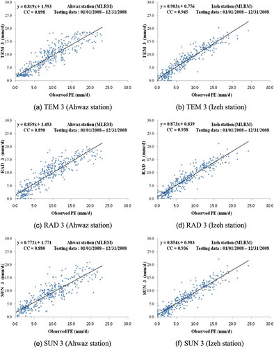
Table 9 Statistical results of the performance of MLRM (testing data).

Station	Input combination	Statistical criteria
		CC	RMSE (mm)	SI	NS
Ahwaz	TEM3	0.898	2.441	0.280	0.807
	RAD3	0.890	2.554	0.293	0.788
	SUN3	0.880	2.648	0.303	0.773
Izeh	TEM3	0.945	1.658	0.224	0.894
	RAD3	0.938	1.758	0.237	0.881
	SUN3	0.936	1.804	0.243	0.874

CONCLUSIONS

In this study, the accuracy of three different soft computing techniques, multilayer perceptron-neural networks model (MLP-NNM), Kohonen self-organizing feature maps-neural networks model (KSOFM-NNM) and gene expression programming (GEP), is investigated for predicting daily PE. Observed PE from the Ahwaz and Izeh stations in Iran are used for training, cross-validation, and testing of MLP-NNM, KSOFM-NNM, and GEP. MLP-NNM, KSOFM-NNM, and GEP are implemented to predict daily PE using the temperature-based, radiation-based, and sunshine duration-based input combinations. This implementation produces high quality predicting for all input combinations. The results show the capability of soft computing models for predicting daily PE. The TEM3 model, whose inputs are T(t – 3), T(t – 2), T(t – 1), T(t), PE(t – 3), PE(t – 2), and PE(t – 1), produces the best results among other input combinations for both stations. The prediction accuracy of soft computing models is found to increase with increasing lag-time intervals for input combinations. KSOFM-NNM slightly outperforms MLP-NNM and GEP, but differences between the results of the three approaches are not significant. The Mann-Whitney U test is performed to compare observed and predicted PE values for the testing data of soft computing models, including TEM3, RAD3, and SUN3. The computed values of z statistic for both stations are not significant for the training data. The null hypothesis, which is that the two independent samples are from the same population, is accepted for both stations. Comparison is also made between the soft computing models and MLRM, which indicates a slight superiority of soft computing models to MLRM.

In the present paper, MLP-NNM, KSOFM-NNM, and GEP models are applied to predict daily PE. Further applications of these models for characterizing other hydrological processes may be applied, e.g. modeling surface water–groundwater interactions, modeling crop response to climate changes, modeling soil–water–air relationships, irrigation scheduling, etc.

Disclosure statement

No potential conflict of interest was reported by the author(s).

REFERENCES

- Allen, R.G., et al., 1998. Crop evapotranspiration guidelines for computing crop water requirements, FAO Irrigation and Drainage, Paper no. 56. Rome: Food and Agriculture Organization of the United Nations.
- ASCE Task Committee on Definition of Criteria for Evaluation of Watershed Models, 1993. Criteria for evaluation of watershed models. Journal of Irrigation and Drainage Engineering, 119 (3), 429–442. doi:10.1061/(ASCE)0733-9437(1993)119:3(429).
- Ayyub, B.M. and McCuen, R.H., 2003. Probability, statistics, and reliability for engineers and scientists. 2nd ed. Boca Raton, FL: Taylor & Francis.
- Bruton, J.M., McClendon, R.W., and Hoogenboom, G., 2000. Estimating daily pan evaporation with artificial neural networks. Transactions of the ASAE, 43 (2), 491–496. doi:10.13031/2013.2730.
- Chang, F.J., et al., 2010. Assessing the effort of meteorological variables for evaporation estimation by self-organizing map neural network. Journal of Hydrology, 384 (1–2), 118–129. doi:10.1016/j.jhydrol.2010.01.016.
- Chang, F.J., Chang, L.C., and Wang, Y.S., 2007. Enforced self-organizing map neural networks for river flood forecasting. Hydrological Processes, 21 (6), 741–749. doi:10.1002/hyp.6262.
- Chang, F.J., Sun, W., and Chung, C.H., 2013. Dynamic factor analysis and artificial neural network for estimating pan evaporation at multiple stations in northern Taiwan. Hydrological Sciences Journal, 58 (4), 813–825. doi:10.1080/02626667.2013.775447.
- Choudhury, B.J., 1999. Evaluation of an empirical equation for annual evaporation using field observations and results from a biophysical model. Journal of Hydrology, 216 (1–2), 99–110. doi:10.1016/S0022-1694(98)00293-5.
- Chow, V.T., Maidment, D.R., and Mays, L.W., 1988. Applied hydrology. NewYork: McGraw-Hill.
- Dawson, C.W. and Wilby, R.L., 2001. Hydrological modelling using artificial neural networks. Progress in Physical Geography, 25 (1), 80–108. doi:10.1177/030913330102500104.
- Ferreira, C., 2001. Gene expression programming: a new adaptive algorithm for solving problems. Complex Systems, 13 (2), 87–129.
- Ferreira, C., 2006. Gene expression programming: mathematical modeling by an artificial intelligence. 2nd ed. Heidelberg: Springer.
- Finch, J.W., 2001. A comparison between measured and modelled open water evaporation from a reservoir in south-east England. Hydrological Processes, 15, 2771–2778. doi:10.1002/hyp.267.
- Gupta, H.V., et al., 2009. Decomposition of the mean squared error and NSE performance criteria: implications for improving hydrological modeling. Journal of Hydrology, 377 (1–2), 80–91. doi:10.1016/j.jhydrol.2009.08.003.
- Guven, A. and Kişi, Ö., 2011. Daily pan evaporation modeling using linear genetic programming technique. Irrigation Science, 29 (2), 135–145. doi:10.1007/s00271-010-0225-5.
- Haykin, S., 2009. Neural networks and learning machines. 3rd ed. Upper Saddle River, NJ: Prentice Hall.
- Hsu, K., et al., 2002. Self-organizing linear output map (SOLO): an artificial neural network suitable for hydrologic modeling and analysis. Water Resources Research, 38 (12), 1302. doi:10.1029/2001WR000795.
- Jain, S.K., Nayak, P.C., and Sudheer, K.P., 2008. Models for estimating evapotranspiration using artificial neural networks, and their physical interpretation. Hydrological Processes, 22 (13), 2225–2234. doi:10.1002/hyp.6819.
- Kay, A.L. and Davies, H.N., 2008. Calculating potential evaporation from climate model data: a source of uncertainty for hydrological climate change impacts. Journal of Hydrology, 358 (3–4), 221–239. doi:10.1016/j.jhydrol.2008.06.005.
- Keskin, M.E. and Terzi, Ö., 2006. Artificial neural network models of daily pan evaporation. Journal of Hydrologic Engineering, 11 (1), 65–70. doi:10.1061/(ASCE)1084-0699(2006)11:1(65).
- Kim, S. and Kim, H.S., 2008. Neural networks and genetic algorithm approach for nonlinear evaporation and evapotranspiration modeling. Journal of Hydrology, 351 (3–4), 299–317. doi:10.1016/j.jhydrol.2007.12.014.
- Kim, S., et al., 2013. Estimating daily pan evaporation using different data-driven methods and lag-time patterns. Water Resources Management, 27 (7), 2267–2286. doi:10.1007/s11269-013-0287-2.
- Kim, S., Kim, J.H., and Park, K.B., 2009. Statistical learning theory for the disaggregation of the climatic data. In: Proceedings of 33rd IAHR Congress 2009, 9–14 August. Vancouver: IAHR, 1154–1162.
- Kim, S., Shiri, J., and Kisi, O., 2012. Pan evaporation modeling using neural computing approach for different climatic zones. Water Resources Management, 26 (11), 3231–3249. doi:10.1007/s11269-012-0069-2.
- Kişi, Ö., 2006. Daily pan evaporation modelling using a neuro-fuzzy computing technique. Journal of Hydrology, 329 (3–4), 636–646. doi:10.1016/j.jhydrol.2006.03.015.
- Kişi, O., 2007. Evapotranspiration modelling from climatic data using a neural computing technique. Hydrological Processes, 21, 1925–1934. doi:10.1002/hyp.6403.
- Kişi, Ö., 2009. Modeling monthly evaporation using two different neural computing techniques. Irrigation Science, 27 (5), 417–430. doi:10.1007/s00271-009-0158-z.
- Kişi, O., Pour-Ali Baba, A., and Shiri, J., 2012. Generalized neurofuzzy models for estimating daily pan evaporation values from weather data. Journal of Irrigation and Drainage Engineering, 138 (4), 349–362. doi:10.1061/(ASCE)IR.1943-4774.0000403.
- Kohonen, T., 1990. The self-organizing map. Proceedings of the IEEE, 78 (9), 1464–1480. doi:10.1109/5.58325.
- Kohonen, T., 2001. Self-organizing maps. NewYork: Springer-Verlag.
- Kottegoda, N.T. and Rosso, R., 1997. Statistics, probability, and reliability for civil and environmental engineers. Singapore: McGraw-Hill.
- Kumar, M., et al., 2002. Estimating evapotranspiration using artificial neural networks. Journal of Irrigation and Drainage Engineering, 128 (4), 224–233. doi:10.1061/(ASCE)0733-9437(2002)128:4(224).
- Legates, D.R. and McCabe, G.J., 1999. Evaluating the use of goodness-of-fit measures in hydrologic and hydroclimatic model validation. Water Resources Research, 35 (1), 233–241. doi:10.1029/1998WR900018.
- Lin, G.F. and Chen, L.H., 2005. Time series forecasting by combining the radial basis function network and the self-organizing map. Hydrological Processes, 19 (10), 1925–1937. doi:10.1002/hyp.5637.
- Lin, G.F. and Chen, L.H., 2006. Identification of homogeneous regions for regional frequency analysis using the self-organizing map. Journal of Hydrology, 324 (1–4), 1–9. doi:10.1016/j.jhydrol.2005.09.009.
- Lin, G.F. and Wu, M.C., 2007. A SOM-based approach to estimating design hyetographs of ungauged sites. Journal of Hydrology, 339 (3–4), 216–226. doi:10.1016/j.jhydrol.2007.03.016.
- Lin, G.F. and Wu, M.C., 2009. A hybrid neural network model for typhoon-rainfall forecasting. Journal of Hydrology, 375 (3–4), 450–458. doi:10.1016/j.jhydrol.2009.06.047.
- McCuen, R.H., 1993. Microcomputer applications in statistical hydrology. Englewood Cliffs, NJ: Prentice Hall.
- Nash, J.E. and Sutcliffe, J.V., 1970. River flow forecasting through conceptual models part I — a discussion of principles. Journal of Hydrology, 10 (3), 282–290. doi:10.1016/0022-1694(70)90255-6.
- NeuroDimension Inc, 2005. Developers of neurosolutions V5.01: neural network simulator. Gainesville, FL: NeuroDimension Incorporated.
- Penman, H.L., 1948. Natural evaporation from open water, bare soil and grass. Proceedings of the Royal Society A: Mathematical, Physical and Engineering Sciences, 193, 120–145. doi:10.1098/rspa.1948.0037.
- Principe, J.C., Euliano, N.R., and Lefebvre, W.C., 2000. Neural and adaptive systems: fundamentals through simulation. NewYork: Wiley, John & Sons, Inc.
- Rosenberry, D.O., et al., 2007. Comparison of 15 evaporation methods applied to a small mountain lake in the northeastern USA. Journal of Hydrology, 340 (3–4), 149–166. doi:10.1016/j.jhydrol.2007.03.018.
- Shiri, J. and Kişi, Ö., 2011. Application of artificial intelligence to estimate daily pan evaporation using available and estimated climatic data in the Khozestan Province (Southwestern Iran). Journal of Irrigation and Drainage Engineering, 137 (7), 412–425. doi:10.1061/(ASCE)IR.1943-4774.0000315.
- Shiri, J., et al., 2011. Estimating daily pan evaporation from climatic data of the state of Illinois, USA using adaptive neuro-fuzzy inference system (ANFIS) and artificial neural network (ANN). Hydrology Research, 42 (6), 491–502. doi:10.2166/nh.2011.020.
- Shiri, J., Marti, P., and Singh, V.P., 2014. Evaluation of gene expression programming approaches for estimating daily pan evaporation through spatial and temporal data scanning. Hydrological Processes, 28 (3), 1215–1225. doi:10.1002/hyp.9669.
- Singh, V.P., Jain, S.K., and Tyagi, A., 2007. Risk and reliability analysis: a handbook for civil and environmental engineers. Reston, VA: ASCE Press.
- Sivakumar, B., Jayawardena, A.W., and Fernando, T.M.K.G., 2002. River flow forecasting: use of phase-space reconstruction and artificial neural networks approaches. Journal of Hydrology, 265 (1–4), 225–245. doi:10.1016/S0022-1694(02)00112-9.
- Sudheer, K.P., et al., 2002. Modelling evaporation using an artificial neural network algorithm. Hydrological Processes, 16 (16), 3189–3202. doi:10.1002/hyp.1096.
- Sudheer, K.P., Gosain, A.K., and Ramasastri, K.S., 2003. Estimating actual evapotranspiration from limited climatic data using neural computing technique. Journal of Irrigation and Drainage Engineering, 129 (3), 214–218. doi:10.1061/(ASCE)0733-9437(2003)129:3(214).
- Tabari, H., Marofi, S., and Sabziparvar, A.A., 2010. Estimation of daily pan evaporation using artificial neural network and multivariate non-linear regression. Irrigation Science, 28 (5), 399–406. doi:10.1007/s00271-009-0201-0.
- Tan, S.B.K., Shuy, E.B., and Chua, L.H.C., 2007. Modelling hourly and daily open-water evaporation rates in areas with an equatorial climate. Hydrological Processes, 21 (4), 486–499. doi:10.1002/hyp.6251.
- Terzi, Ö. and Erol Keskin, M., 2005. Evaporation estimation using gene expression programming. Journal of Applied Sciences, 5 (3), 508–512. doi:10.3923/jas.2005.508.512.
- Tokar, A.S. and Johnson, P.A., 1999. Rainfall-runoff modeling using artificial neural networks. Journal of Hydrologic Engineering, 4 (3), 232–239. doi:10.1061/(ASCE)1084-0699(1999)4:3(232).
- Vallet-Coulomb, C., et al., 2001. Lake evaporation estimates in tropical Africa (Lake Ziway, Ethiopia). Journal of Hydrology, 245 (1–4), 1–18. doi:10.1016/S0022-1694(01)00341-9.