Hydrologic simulation approach for El Niño Southern Oscillation (ENSO)-affected watershed with limited raingauge stations

ABSTRACT

Since the performance of hydrological models relies on numerous factors, the selection of an appropriate modeling approach for hydrological study has always been a crucial issue. The major objective of this research is to demonstrate that data-driven models such as the Adaptive Neuro-Fuzzy Inference system (ANFIS) are more suitable in a region where spatially distributed precipitation datasets are not available. Since precipitation has a teleconnection with the El Niño Southern Oscillation (ENSO) in different parts of the world, the sea surface temperatures (SSTs) and sea level pressures (SLPs) of the equatorial Pacific can be expected to act as surrogates for the precipitation if there are insufficient raingauge stations in the watershed. Moreover, in contrast to conceptual and physically-based models, data driven models can incorporate SST and SLP in their input vectors, and hence additional forcing of SST with precipitation has been experimented with in past studies. Therefore, our second objective is to test whether the additional forcing of SST and SLP will improve the hydrologic simulation. For this, various ANFIS models for the winter season were developed considering 10 raingauge stations situated at various locations in the watershed. Rainfall from each raingauge station was considered in the ANFIS model one at a time with and without SST/SLP. The results show that the performance of the ANFIS model improved with the additional fusion of SST and SLP, especially when a raingauge station from a remote location was considered. However, this improvement was observed when the analysis was primarily focused on the winter season which is a period with a strong ENSO signal.

Editor D. Koutsoyiannis Associate editor L. See

KEYWORDS:

• ENSO
• ANN
• fuzzy logic
• ANFIS
• spatial variability
• hydrologic modeling

1 Introduction

Hydrologic simulation is one of the most important topics in hydrology due to its wide application, e.g. in flood and drought forecasting and in the design of hydraulic structures. Furthermore, hydrologic simulation is a complex process, relying on various linear and nonlinear parameters (Singh 1988). Accordingly, various approaches of modeling such as process-based models, conceptual models, or data-driven/black-box models (Jayawardena et al. 2006) have been proposed for streamflow simulations for different historical time periods. Different studies in the past have reported that the performance of the models varies according to several factors, including the availability of the data, user’s knowledge, the accuracy needed and the availability of time and resources. Therefore, it is difficult to generalize regarding the most suitable modeling approach (Jayawardena et al. 2006).

Irrespective of the modelling approach used, hydrologic simulation is affected significantly by the quality of the precipitation data (Sharma et al. 2012a). On the one hand, a fully physically-based model representing complex land use and soil characteristics with detailed input is also not capable of simulating the streamflow well if the spatial variability of precipitation is not adequately incorporated. On the other hand, spatially distributed rainfall data needed for physically-based or distributed and semi-distributed hydrologic models are rarely available. Generally, it is difficult to capture the spatial variability of the rainfall in watershed modeling unless an adequate number of raingauge stations is available (Sharma et al. 2012a). In addition, with the conventional method of using tipping bucket raingauges, the readings are actually point measurements and do not capture the actual rainfall occurring on the surface unless a dense enough network of raingauges is available.

Since variations in the sea surface temperature (SST) and sea level pressure (SLP) of various regions of the equatorial Pacific have significant influence on inter-annual variation of precipitation and temperature in different parts of the world (Piechota and Dracup 1996, Chiew et al. 1998, Rajagopalan and Lall 1998, Barsugli et al. 1999, McCabe and Dettinger 1999, Kulkarni 2000, Pascual et al. 2000, Hansen et al. 2001, Roy 2006, Keener et al. 2007), SST and SLP can be additional forcing variables in data-driven models to improve hydrologic simulation. This variation in SST and SLP along the equatorial pacific is called the El Niño Southern Oscillation (ENSO).

Different ENSO phases (La Niña, El Niño and Neutral) are identified using various ENSO indicators (SSTs and SLPs) in the equatorial Pacific Ocean. Considering the potential teleconnection between streamflow and ENSO indicators, it may be possible to explicitly utilize these indicators in rainfall–runoff modeling. In other words, SST and SLP can be expected to act as surrogates for the precipitation, particularly for a watershed where spatially distributed precipitation data are not available. However, physically-based and conceptual models cannot incorporate SST and SLP data as an input, and hence data-driven models such as artificial neural networks (ANNs) and fuzzy logic-based models could be appropriate choices in such cases.

Although ANN and fuzzy logic have been proven to be effective and useful when compared with conventional modeling due to their ability to handle large amounts of data, especially when the underlying physical processes are not understood or parameterized (Nayak et al. 2004), scientists have shown an interest in combining these two models. For example, a neuro-fuzzy system known as an Adaptive Neuro-Fuzzy Inference System (ANFIS) (Jang 1993) has been developed and extensively applied in hydrological (Mukerji et al. 2009, Pramanik and Panda 2009) and water quality modeling (Yan et al. 2010).

This study explored the suitability of ANFIS models for simulating streamflow using potential ENSO indicators (SST and SLP) of the equatorial Pacific as input variables. Few studies in the past have used ENSO indicators in data-driven models (Khalil et al. 2005, Makkeasorn et al. 2008) for hydrologic study. Thus, the objectives of this paper are to: (1) demonstrate that the ANFIS model is a suitable choice for ENSO affected watersheds with limited raingauge stations, and (2) incorporate SST and SLP in an ANFIS model, comparing the performance with and without these additional inputs.

2 Theoretical background

ENSO, which is measured using various ENSO indicators, is considered as one of the most reliable phenomena for relating inter-annual climate variability in streamflow at both local and global scales (Ropelewski and Halpert 1986). For ENSO prediction, the US National Oceanic and Atmospheric Administration (NOAA) constantly monitors the Niño 3.4 region which is located between 5^oN–5^oS and 120^o–170^oW in the equatorial Pacific. An ENSO phase is classified based on the Niño 3.4 index which is calculated based on a 3-month running mean of ERSST.v3b SST anomalies in this region (Trenberth and Stepaniak 2001). ENSO indicators are incorporated in the ANFIS model which is described in the following section.

3 ANFIS

ANFIS is a multi-layer feed-forward network that utilizes a neural network and fuzzy logic to map an input vector to an output vector by using back-propagation or a combined algorithm. A generic example of an ANFIS model using two inputs and one output is demonstrated in Fig. 1. This model is comprised of five layers with two rules, and two membership functions (MFs) for each input (Fig. 1).

Figure 1. ANFIS architecture for two inputs (X and Y) with two rules and two membership functions (P1, P2 and Q1, Q2) for each rule.

The ANFIS model comprising two fuzzy if–then rules can be written as follows:

(1)

(2)

where P1 and P2 are the MFs for input X, Q1 and Q2 are the MFs for input Y, a₁, b₁, r₁ and a₂, b₂, r₂ are the parameters to be determined for the output function. The brief operation of the ANFIS model is explained as follows: Layer 1 In this layer, each node with membership functions is called an adaptive node.

(3)

(4)

Here, X and Y are inputs, represents the membership function and P_i and Q_i–2 are fuzzy sets.

Layer 2 In this layer, a single output representing the result of the predecessor (firing strength) of that rule is obtained. Hence, the outputs O²_i of this layer can be expressed as:

(5)

Layer 3 In this layer, every node is labeled N, and the ratio of firing strength corresponding to each ith rule to the summation of firing strength that corresponds to all rules is computed:

(6)

Layer 4 In this layer, the input contribution of each ith rule for the output of the model is computed using:

(7)

where is the output from Layer 3 and [a_i, b_i, r_i] are the model parameters.

Layer 5 The final output is computed as the combination of all receiving signals:

(8)

The ANFIS model applies a hybrid-learning algorithm (i.e. the combination of the gradient descent method and the least-squares method) to update the model parameters. In order to reduce the number of rules and for effective partitioning, several clustering methods have been suggested to organize the data and construct the rules. Some of the most widely used approaches are grid partitioning (Jang and Sun 1995), the subtractive clustering algorithm (SCA) (Chiu 1996), and fuzzy C-means (FCM) (Dunn 1973).

3.1 Study area and data

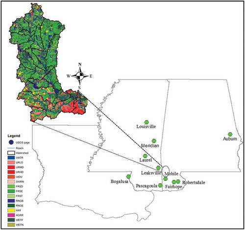
The study area is located in the Chickasaw Creek watershed (Fig. 2) of Mobile County, southern Alabama (USA), in the Mobile River basin. The watershed is 714 km² in size and starts at Citronelle, AL in the north, and eventually drains into Mobile Bay. The watershed is dominated by coastal plain geology with an elevation ranging from 0 to 13.11 m above mean sea level. The average annual precipitation in the watershed (1651 mm) is relatively higher than in other parts of Alabama. Air temperature and precipitation datasets were available from the weather station at Mobile Regional Airport (Coop ID-015478), downloaded from the National Climatic Data Center (NCDC). This is the closest raingauge station to the watershed, which is still 32 km away from the watershed boundary. Streamflow data, recorded since 1952, were available at the USGS gauge (02471001) which drains 357 km² of the watershed.

Figure 2. Chickasaw Creek watershed in Mobile County, southern Alabama, USA, showing the USGS gauging station and land-use distribution within the watershed. The land-use classification is as per NLCD land-use categories.

The climate of this region, especially the study area, is highly affected by ENSO, which has been reported in various past studies (Hansen et al. 2001, Sharma et al. 2012b). Winter is characterized by high precipitation and streamflow, and low temperature during the El Niño phase, which is just opposite to the conditions during La Niña, as shown in Fig. 3. The ENSO signal is comparatively better in winter and spring compared to summer. Similarly, the ENSO correlation with precipitation and temperature is opposite in nature during the period from August to October compared to winter and spring (Fig. 4).

Figure 3. Variation of monthly average precipitation and temperature in the El Niño and La Niña phases for (a) the winter (January–March) season and (b) the spring (April–June) season.

Figure 4. Pattern of streamflow in two different ENSO phases.

Average SST, SLP differences (between Tahiti and Darwin) and the trade wind index (Lukas et al. 1984) in the Niño 3.4 region (5°N–5°S, 120°W–170°W) (Trenberth and Stepaniak 2001) were available since 1950, and downloaded from NOAA’s NCDC and National Center for Environment Prediction (NCEP) website. The data used in the study with their sources and formats are reported in Table 1.

Table 1. Data used in the study with their sources and format.

Data	Source	Additional information
Weather gauge station	NOAA, National Climatic Data Center, http://ncdc.noaa.gov	Coop ID-015478
Streamflow	www.al.water.usgs.gov	(USGS gage 02471001)
Hydrologic (stream network) data	www.aces.edu/waterquality/gisdata
GIS layers/TIGER files	www.AlabamaView.org

4 Methodology

4.1 Estimation of parameters

Based on the simple architecture of the ANFIS model (designed for the given input parameters), the ANFIS structure was further extended to several other inputs. For the present study, SF = f (SST, SLP, T, PCP), where SF, PCP and T are streamflow (m³/s), precipitation (mm) and air temperature (°C), respectively. For simplicity, an example of an ANFIS having two inputs with two rules is presented here for illustration. Assuming P1:P2 and Q1:Q2 are the respective membership functions for two input variables (SST and PCP) and a₁:b₁, a₂:b₂ are the model parameters associated with the output function, then the resultant output is computed as linear combinations of subsequent parameters. The equation to predict SF_i (output), i.e. the streamflow at time t₁, can be simplified as follows:

(9)

All equations to predict the streamflow time series (SF₁, SF₂ … SF_n) may be arranged in matrix form as follows:

(10)

where Z, as an unknown model parameter matrix, was derived from training datasets solving the following equation:

(11)

where is the inverse of matrix A and is the transpose of matrix A. In order to solve this matrix, we used the hybrid learning algorithm which combines both the least-squared method and the back-propagation algorithm. The hybrid approach trains the data rapidly and also converges much faster.

4.2 Input data selection

The selection of input variables is a crucial part of ANFIS modeling. Optimum inputs should be selected in order to best capture the input and output relation. Since streamflow of this month may also be associated with the temperature and precipitation of an earlier month, the cross-correlation technique was used to decide on the appropriate inputs. Moreover, streamflow is an integral form of the quick response component of the watershed, i.e. surface runoff, and the slow response component, i.e. baseflow. Baseflow might be associated with the precipitation of many time steps ahead, whereas surface runoff is associated with the current time step. Therefore, it is always preferable to partition the streamflow into baseflow (BF) and surface runoff (SR) components. Accordingly, we used the baseflow filter program (Lim et al. 2005) (https://engineering.purdue.edu/~what/), developed at Purdue University for online hydrograph separation. We used the Recursive Digital Filter method to derive separate SR and BF datasets from streamflow data to develop separate SR and BF models. The input variables for the SR model were estimated surface runoff, temperature, SST and SLP at different lead times (Table 2). The estimated surface runoff was computed from precipitation using the SCS curve number equation (Bosznay 1989). The curve number (CN) was estimated based on the SSURGO soil (SSURGO 2010) database and the 2001 land cover dataset (NLCD 2010). Likewise, the model input variables for the BF model were SST, SLP, air temperature and precipitation at different lead times (Table 2).

Table 2. Input variables for the ANFIS model (monthly data).

Model	Model inputs
SR Model	SST(t-1)	SLP(t)	T(t-1)	T(t)	SRE(t-1)	SRE(t)
BF Model	SST(t)	SLP(t)	T(t-1)	PCP(t-1)	PCP(t)

Note: SR_E, T(t), PCP(t), and SST(t), SLP(t) denote ‘estimated surface runoff’, temperature, precipitation, sea surface temperature, and sea level pressure difference between Tahiti and Darwin in month ‘t’, respectively.

In the next step, multiple linear regression (MLR) models were fit to different sets of inputs in order to identify the significant model inputs. It was important to evaluate whether SSTs and SLPs were the significant model inputs in addition to temperature and precipitation. In fact, precipitation and temperature are also affected by SST and SLP. One way to see whether the additional forcing of SST and SLP are beneficial is to evaluate the adjusted R² from the MLR model. If the additional forcing of SST and SLP is not beneficial, those inputs may not be statistically significant in the MLR model, and there will be no additional improvement in the adjusted R². Even though MLR and ANFIS are two different modeling approaches, the parameters that are not statistically significant in MLR may not be appropriate inputs in the ANFIS model as well. For this reason, an MLR model was developed, and the model depicted that the parameters were significant for P < 0.1. A sensitivity analysis was also conducted by excluding those parameters one at a time from the input vectors and evaluating the performance. The results suggested that SST and SLP were two of the most sensitive model inputs. The optimal lead time and the number of inputs were decided after the sensitivity analysis. Various combinations of inputs were experimented with at different lead times to determine the best inputs. Any additional inputs beyond the optimum sets did not improve the model performance.

The analysis suggested that both SST and SLP data were important, especially in the seasons that ENSO showed a clear signature with streamflow (winter, spring and early fall). Each model was comprised of separate SR and BF models. The ANFIS model, without SST and SLP, was developed to evaluate the importance of SST and SLP inputs.

4.3 Model development and implementation

The most sensitive sets of inputs giving the best result in the MLR model were employed in the ANFIS model. The final form of the equation for the SR ANFIS model is given as:

(12)

where SR is monthly average surface runoff in m³/s, t is the monthly time step, is the estimated surface runoff using the SCS curve number method based on precipitation, land use/land cover and soil. The model inputs for both the SR and BF models are also presented in Table 2. The ANFIS model was extended to a daily scale with some modification in its input datasets. For the SR model, while simulating at a daily scale, we used the same inputs that we used for the monthly SR model. However, baseflow at the daily scale may depend on the precipitation characteristics of the preceding few weeks due to the time lag of the groundwater contribution. Therefore, the combination of precipitation sets at different lead times were experimented with in the ANFIS model until the model performance improved.

The MATLAB fuzzy logic toolbox was selected for ANFIS simulation using 50 years of observed data; 80% of the total data were used for model training, 10% for model validation and 10% for model testing. Both SCA and FCM clustering methods were experimented with for the selection of the initial model parameters. For this particular study and the given datasets, SCA was found to be more suitable to cluster the datasets because it provided consistently better performance in training, validation and testing. The parameters to be fixed for SCA were clustering radius, acceptance ratio and rejection ratio. We varied the clustering radius from 0.3 to 1 using 0.05 as the step size to determine the optimal parameters which were ascertained by minimizing the root mean squared error. Other parameters, such as the number of epochs, range of influence of the cluster center, the acceptance ratio, and the rejection ratio of the model, were optimally ascertained through repeated trial and error. In order to avoid overtraining of the model, the simulation was stopped when the validation error started increasing.

The performance of each ANFIS model was measured via three non-dimensional measures: R² (coefficient of determination), the Nash-Sutcliffe efficiency (NSE) (Nash and Sutcliffe 1970), and the mass balance error (MBE); and the dimensional measure, root mean square error (RMSE). Details of these performance measures are described in many other articles (Abrahart and See 2007, Dawson et al. 2007, Moriasi et al. 2007).

Since our second objective was to test whether the SST and SLP improve streamflow simulation or not, several winter season ANFIS models were developed. We employed three techniques to evaluate the additional benefit of SST and SLP for streamflow simulation. First, we compared the performance of the ANFIS model including SST and SLP with one excluding SST and SLP from its input vector for the entire season in both SR and BR models. Secondly, 20 ANFIS models were developed for the winter season with and without SST/SLP by replacing the raingauge considered for the watershed (Mobile, Coop ID-015478) by other rainfall stations at different locations, one after the other. Third, 20 additional ANFIS models were developed with and without SST/SLP considering only La Niña and El Niño periods. Since Neutral period characteristics are associated with the immediately preceding season, the Neutral period does not show any trend. That is, the Neutral period followed by El Niño is different to a Neutral period followed by La Niña. Therefore, in the third case, we developed the model using only the La Niña and El Niño phases to further diagnose how SST/SLP play a role in simulation, particularly when it enters the La Niña and El Niño phases. For the second and third cases, we developed models with 10 raingauge stations as inputs, including the raingauge considered for the watershed, and then randomly selected nine additional rainfall stations at various locations in three different States of Alabama, Mississippi and Louisiana with closest proximity to the watershed, which furnish long-term climate data since the 1950s (Fig. 2). These analyses were conducted in order to evaluate the model performance with the rainfall located at a significant distance from the watershed. The underlying assumption was that the SST and SLP could be helpful for satisfactory simulation even if the spatially distributed precipitation was not available. Therefore, in each case, the raingauge station considered for the watershed was replaced by those additional raingauge stations one at a time, and the model performance was evaluated with and without SST/SLP. The reason for developing a winter season model is to test the sensitivity of SST and SLP during the winter period because ENSO has a clear signature with precipitation and temperature in winter. The ENSO signal is comparatively stronger in the winter and spring seasons in this region (Fig. 3). Also, the ENSO signal is clear in August to October but opposite in characteristics to that of winter and spring (Fig. 4).

Since we had to develop 40 different ANFIS models for the second and third analyses, we limited our analysis to the winter seasons, and also used temperature, precipitation, SST and SLP at the current time level as inputs. This is because the effect of ENSO indicators may not be distinct due to too many conflicting variables if the inputs at different lag times were considered. Moreover, our objective in this analysis was to verify that SST and SLP are beneficial for streamflow simulation. Therefore, we developed a single SF model due to the computational efforts required, particularly for the second and third analyses. The second and third analyses, which comprise a type of sensitivity analysis of the ANFIS model, were also developed using 80% training data, 10% validation and 10% testing data.

5 Results and discussion

5.1 Performance of the ANFIS model

The overall performance of the simulated streamflow model, i.e. the combined SR and BF models, against observed data, is presented in Table 3. The model simulated streamflow with satisfactory performance in each stage of training, validation and testing (Table 3). From visual inspection, it can be concluded that the model simulation matched the observed monthly streamflow well (Fig. 5). Furthermore, the ANFIS model simulation was at a daily time step. It is interesting to note that SLP, SST and SST(t – 1) were the most sensitive inputs for the BF model at a daily temporal resolution as well. The overall ANFIS model performance including training, validation and testing was also satisfactory at a daily temporal resolution (NSE = 0.68, MBE = 0.6%, RMSE = 7 m³/s).

Table 3. Performance of the ANFIS model in different modeling stages (monthly simulation from 1952 to 2002).

Statistics	Streamflow simulation
	Training (1952–1989)	Validation (1990–1996)	Testing (1997–2002)
RMSE (m^3/s)	2.63	2.37	3.7
NSE	0.8	0.85	0.74
MBE	0%	3.8%	8.8%

Figure 5. Monthly streamflow simulated for 52 years using the ANFIS model compared with observed monthly streamflow.

The ANFIS model was able to capture some of the highest flow associated with ENSO events of January 1954 (El Niño), April 1980 (Neutral), May 1991 (El Niño), July 1997 (El Niño) and September 1998 (La Niña) (Fig. 5). Because SST and SLP were directly implemented in the ANFIS model, it was interesting for us to explore how this model would simulate streamflow at corresponding major historic ENSO events from 1950 onwards, which are listed in Table 4. The ANFIS model performance was satisfactory for different ENSO events (Table 5) due to the training of the ANFIS model with long-term datasets. The long time series of ANFIS model simulation of historic ENSO events is shown in Fig. 5.

Table 4. El Niño and La Niña years (December–April) from 1950 to 2003.

La Niña year	El Niño year
1950	1958
1951	1966
1955	1969
1956	1973
1968	1983
1971	1987
1974	1988
1975	1992
1976	1995
1985	1998
1989	2003
1996
1999
2000

Table 5. ANFIS model performance for 25 ENSO events (monthly simulation).

Statistics		ANFIS-simulated
For La Niña and El Niño events (since 1952)
NSE		0.83
MBE		3.10
R^2		0.83
14 La Niña events (Table 7)
NSE		0.86
MBE		6%
R^2		0.87
11 El Niño events (Table 7)
NSE		0.76
MBE		−3.12%
R^2		0.77

Since SST, SLP and the trade wind index are the parameters related to the basic ENSO phenomenon in the equatorial Pacific, the trade wind index was also a sensitive input for the model developed from 1979 to 2011 (not shown). This indicates that hydrologic analysis in ENSO-affected coastal areas can be better addressed using SST, SLP and the trade wind index. Because we wanted to run the model on 50 years of data to evaluate the performance of the model in different ENSO events, we could not include the trade wind index as model inputs as these data were available only after 1979.

The performance of the ANFIS model, for the given datasets in this watershed, has been compared with a physically-based model, the Loading Simulation Program C⁺⁺⁺ (LSPC), and reported in Sharma (2012). The comprehensive model comparison of ANFIS with the LSPC model suggests that ANFIS can perform equally or better than this physically-based watershed model, especially when sufficient raingauge stations are not available (Sharma 2012).

5.2 ANFIS model and ENSO indicators

Having analyzed the model performance at different scales for different events, it can be concluded that the ANFIS model can simulate the watershed response well, partly due to the direct incorporation of the dominant ENSO phenomenon, and partly due to the ANFIS model skill in using ENSO inputs. Moreover, it was important to confirm that the improvement of the model simulation was due to the application of SST/SLP. This was shown in three ways. First, we assessed the performance of the ANFIS model with and without SST and SLP in the input vector, and found that the ANFIS model tended to perform better when SST and SLP were included (Table 6). Since the ENSO characteristic is completely different from season to season (Fig. 4), the model developed for the entire season using SST did not improve the results significantly. This is mainly because SST/SLP has a positive correlation with streamflow during winter and spring but the opposite correlation with streamflow from August to October, i.e. separate models should be trained in winter, spring and from August to October. For this reason, the second and third analyses were conducted primarily for the winter season in order to see the actual effect of SST/SLP on the streamflow simulation.

Table 6. Performance of the ANFIS model during 50 years simulation at monthly time step.

Statistics	ANFIS (with SST and SLP)	ANFIS (without SST and SLP)
NSE	0.79	0.74
MBE	0.60%	1.27%
R^2	0.79	0.74

For the second case, we developed models with and without SST/SLP for the winter season, considering the precipitation from each raingauge station one at a time. For example, we replaced the watershed raingauge station (Mobile, Coop ID-015478) with the precipitation from Fairhope (Fig. 2). Unsurprisingly the simulation performance was poor as it was Fairhope is located about 37 km away from the Mobile (Coop ID 015478) raingauge station. However, when SST/SLP was considered as an input in addition to the Fairhope precipitation, the model performance improved (Table 7). In fact, this model performance is almost similar to that obtained when the Mobile (Coop ID-015478) raingauge station was used without SST/SLP. This indicates that precipitation from the farthest location can also be utilized, resulting in similar model performance, provided that the SST and SLP are incorporated. Similarly, we used precipitation data from a raingauge station located in mid Alabama (Auburn), which is 341.5 km from the watershed raingauge station (Table 7). Since the actual rainfall characteristic of the watershed was not represented by the Auburn rainfall, the model simulation was poor. However, when SST/SLP was added to the same precipitation from Auburn, the overall model performance improved (Table 7). Similarly, we used rainfall data from Louisville and Meridian, which were the second and third furthest locations from the watershed (Fig. 2), respectively. In each case, the model performance improved with the additional forcing of SST and SLP. Despite being closer to the watershed raingauge station, Laurel and Leakesville (135 and 60 km away) (Table 7) did not show better performance without SST and SLP, especially compared to one of the farthest raingauge stations, Auburn. However, performance improved in both cases after incorporating SST and SLP. The third remote location was Meridian, where the performance without SST and SLP was not satisfactory. Even though this station is nearer than Auburn, the performance is not better. One reason could be the precipitation quality of the station. At times, two raingauge stations which are located in virtually the same place, but monitored and operated by different agencies, can show poor correlations (Sharma et al. 2012a) indicating that a raingauge station may not represent the true precipitation in the watershed if it is not maintained properly. Moreover, poor recording and missing data are quite often found in raingauge stations. In this context, the additional forcing of SST and SLP became crucial to improving the simulation when using precipitation data from the Meridian station. The performance improved in the majority of cases, and the effect of SST and SLP was important, especially when raingauge stations were considered from the remotest locations.

Table 7. Sensitivity analysis of the ANFIS model performance measured through R² using precipitation from various raingauge stations for winter season with and without SST/SLP.

Stations	With SST/SLP		Without SST/SLP		Distance from Mobile station (km)
	Training	Validation/testing	Training	Validation/testing
Bogalusa	0.82	0.1	0..54	0.00	154.70
Fairhope, AL	0.77	0.32	0.63	0.13	36.70
Laurel	0.73	0.06	0.44	0.02	135.70
Lakesville	0.75	0.35	0.60	0.08	60.00
Louisville	0.86	0.22	0.68	0.04	282.40
Meridian	0.84	0.26	0.52	0.07	187.40
Mobile, AL	0.91	0.52	0.70	0.64	0.00
Pascagoula, MS	0.72	0.58	0.56	0.38	40.90
Robertsdale	0.74	0.34	0.50	0.33	54.50
Auburn	0.68	0.28	0.60	0.06	341.50

Even though the effect of SST/SLP improved the model performance in the majority of cases, we considered only El Niño and La Niña phases to further diagnose the effect of SST when precipitation from different locations was considered. For the third analysis, we repeated the method but with the data taken from the El Niño and La Niña period, because the Neutral period is associated with tremendous uncertainty. The performance when using rainfall data from Pascagoula, Louisville, Leaksville and Laurel was poor, especially when ENSO indicators were removed from the input vectors (Table 8). However, the performance improved when ENSO indicators were incorporated. This was true for precipitation from the majority of the stations indicating that the model tends to perform better when incorporating SST and SLP (Table 8).

In addition, the winter season simulation was tested using a MLR model. It was found that the model improved for the winter season due to the direct application of SST and SLP. We want to clearly infer that application of SST and SLP is beneficial only for a period when ENSO shows a stronger signature with streamflow. Readers may also refer to the comprehensive analysis regarding the importance of SST in data-driven models in ENSO-affected regions (Sharma 2012). Since ENSO has a better signature with precipitation in winter and spring but not in summer in the study watershed (Sharma et al. 2012b), we only tested the model performance with and without SST/SLP for these seasons.

Table 8. Sensitivity analysis of the ANFIS model performance measured through R² using precipitation from various raingauge stations during the El Niño and La Niña periods of winter with and without SST/SLP.

Stations	With SST/SLP		Without SST/SLP
	Training	Validation/testing	Training	Validation/testing
Bogalusa	0.44	0.54	0.42	0.51
Fairhope, AL	0.66	0.6	0.54	0.57
Laurel	0.45	0.35	0.35	0.32
Leakesville	0.49	0.38	0.48	0.32
Louisville	0.42	0.14	0.25	0.15
Meridian	0.46	0.36	0.30	0.24
Mobile, Al	0.65	0.58	0.62	0.53
Pascagoula, MS	0.43	0.51	0.37	0.43
Robertsdale	0.41	0.51	0.43	0.44
Auburn	0.52	0.34	0.43	0.18

Since there is only one raingauge station (Mobile, Coop ID-015478) in the Chickasaw Creek watershed, it is clear that the model developed for the entire season considering only one raingauge station suffers from the lack of spatially distributed precipitation data. This was clear through close inspection of precipitation and corresponding streamflow over a long period of record. Some of the streamflow events did not correspond to the observed precipitation. There could be many reasons for the unusual streamflow for a given precipitation record. Some of the major reasons are: (1) the precipitation recorded at the station was erroneous on that day, (2) the precipitation measured at the station did not match the actual precipitation that occurred in the watershed, (3) there was an error while measuring the observed data (e.g. precipitation and streamflow). SST and SLP are physically associated and bring about rainfall variation. Hence, inclusion of these variables may not be required. However, the precipitation input in this model did not adequately represent the actual precipitation characteristic of the watershed. Hence, the underlying assumption was that incorporating SST and SLP would be helpful to eliminate the error associated with point measurements of rainfall, any recording errors in the precipitation, and missing precipitation data being filled with data from the other precipitation stations.

6 Summary and conclusion

In this paper, we incorporated the SST and SLP difference between Tahiti and Darwin directly in the ANFIS model as model inputs and investigated model performance over 50 years of simulation. The performance of the ANFIS model was comprehensively evaluated with observed streamflow using different statistical criteria at different periods and seasons. Moreover, observed and simulated streamflow were compared in different La Niña and El Niño events throughout the 50-year simulation period. The model simulated the monthly streamflow satisfactorily, with reasonable accuracy. ANFIS models were developed with and without SST and SLP in order to evaluate the influence of additional forcing of SST and SLP in data-driven models. Since the ENSO characteristics are opposite in nature from season to season, the model developed for the entire season did not improve significantly. However, the performance improved during the ENSO period in the winter season. The relevance of applying SST and SLP was tested using precipitation data at various locations, developing 20 ANFIS models and considering 10 raingauge stations. The performance of the ANFIS model improved when SST and SLP were applied irrespective of the raingauge station locations. Moreover, the capability of the ANFIS model to capture the low and high flows during winter La Niña and El Niño events suggest the application of SST and SLP is useful for long-term continuous streamflow simulation. This research opens a new window for future studies to develop neuro-fuzzy computational techniques by using long-term recorded climate data in the equatorial Pacific for rainfall–runoff modeling to capture the dominant climate pattern, ENSO. As discussed in different studies reported in the literature, there are various modeling approaches and the supremacy of one modeling approach over another cannot be generalized. However, this research highlights the application of data-driven modeling approaches using SST and SLP data in ENSO-affected coastal regions, which is especially beneficial when the number of raingauge stations is not sufficient. More importantly, it provides a viable alternative for streamflow simulation and justifies the relevance of traditional data-driven modeling approaches.

Since the rainfall–runoff modeling that is applicable in much of the US is not applicable to the coastal plain (Sheridan et al. 2002), this approach is much more relevant for coastal watersheds that are affected by ENSO climate patterns.

Acknowledgements

The authors would like to acknowledge the corrections and suggestions made by the anonymous reviewers and the associate editor to improve this manuscript. The comments of the reviewers and associate editor were very helpful in addressing numerous issues which were overlooked in our initial submission.

Disclosure statement

No potential conflict of interest was reported by the authors.

References

- Abrahart, R. and See, L., 2007. Neural network modelling of non-linear hydrological relationships. Hydrology & Earth System Sciences, 11, 5.
- Barsugli, J.J., et al., 1999. The effect of the 1997/98 El Niño on individual large-scale weather events. Bulletin of the American Meteorological Society, 80, 1399–1411. doi:10.1175/1520-0477(1999)080<1399:TEOTEN>2.0.CO;2
- Bosznay, M., 1989. Generalization of SCS curve number method. Journal of Irrigation and Drainage Engineering, 115, 139–144. doi:10.1061/(ASCE)0733-9437(1989)115:1(139)
- Chiew, F., et al., 1998. El Niño/Southern Oscillation and Australian rainfall, streamflow and drought: links and potential for forecasting. Journal of Hydrology, 204 (1–4), 138–149. doi:10.1016/S0022-1694(97)00121-2
- Chiu, S., ed., 1996. Method and software for extracting fuzzy classification rules by subtractive clustering. In: Biennial conference of the North American Fuzzy Information Processing Society (NAFIPS), 19–22 January, Berkeley, CA. IEEE.
- Dawson, C.W., Abrahart, R.J., and See, L.M., 2007. HydroTest: a web-based toolbox of statistical measures for the standardised assessment of hydrological forecasts. Environmental Modelling & Software, 27, 1034–1052.
- Dunn, J.C., 1973. A fuzzy relative of the ISODATA process and its use in detecting compact well-separated clusters. Journal of Cybernetics, 3, 32–57.
- Hansen, J., et al., 2001. El Niño-Southern Oscillation impacts on crop production in the southeast United States. ASA Special Publication, 63, 55–76.
- Jang, J.S.R., 1993. ANFIS: Adaptive-network-based fuzzy inference system. IEEE Transactions on Systems, Man, and Cybernetics, 23 (3), 665–685. doi:10.1109/21.256541
- Jang, J.S.R. and Sun, C.T., 1995. Neuro-fuzzy modeling and control. Proceedings of the IEEE, 83 (3), 378–406. doi:10.1109/5.364486
- Jayawardena, A., Muttil, N., and Lee, J., 2006. Comparative analysis of data-driven and GIS-based conceptual rainfall–runoff model. Journal of Hydrologic Engineering, 11, 1–11. doi:10.1061/(ASCE)1084-0699(2006)11:1(1)
- Keener, V., et al., 2007. Effects of El Niño/Southern Oscillation on simulated phosphorus loading in South Florida. Transactions of the ASAE, 50 (6), 2081–2089.
- Khalil, A.F., et al., 2005. Basin scale water management and forecasting using artificial neural networks1. JAWRA Journal of the American Water Resources Association, 41 (1), 195–208. doi:10.1111/j.1752-1688.2005.tb03728.x
- Kulkarni, J., 2000. Wavelet analysis of the association between the southern oscillation and the Indian summer monsoon. International Journal of Climatology, 20 (1), 89–104. doi:10.1002/(SICI)1097-0088(200001)20:1<89::AID-JOC458>3.0.CO;2-W
- Lim, K.J., et al., 2005. Automated Web Gis based hydrograph analysis tool, WHAT1. JAWRA Journal of the American Water Resources Association, 41 (6), 1407–1416. doi:10.1111/j.1752-1688.2005.tb03808.x
- Lukas, R., Hayes, S.P., and Wyrtki, K., 1984. Equatorial sea level response during the 1982–1983 El Niño. Journal of Geophysical Research: Oceans (1978–2012), 89 (C6), 10425–10430. doi:10.1029/JC089iC06p10425
- Makkeasorn, A., Chang, N.-B., and Zhou, X., 2008. Short-term streamflow forecasting with global climate change implications – a comparative study between genetic programming and neural network models. Journal of Hydrology, 352 (3–4), 336–354. doi:10.1016/j.jhydrol.2008.01.023
- McCabe, G.J. and Dettinger, M.D., 1999. Decadal variations in the strength of ENSO teleconnections with precipitation in the western United States. International Journal of Climatology, 19 (13), 1399–1410. doi:10.1002/(SICI)1097-0088(19991115)19:13<1399::AID-JOC457>3.0.CO;2-A
- Moriasi, D., et al., 2007. Model evaluation guidelines for systematic quantification of accuracy in watershed simulations. Transactions of the ASABE, 50 (3), 885–900.
- Mukerji, A., Chatterjee, C., and Raghuwanshi, N.S., 2009. Flood forecasting using ANN, neuro-fuzzy, and neuro-GA models. Journal of Hydrologic Engineering, 14, 647–652. doi:10.1061/(ASCE)HE.1943-5584.0000040
- Nash, J. and Sutcliffe, J., 1970. River flow forecasting through conceptual models part I – a discussion of principles. Journal of Hydrology, 10 (3), 282–290. doi:10.1016/0022-1694(70)90255-6
- Nayak, P., et al., 2004. A neuro-fuzzy computing technique for modeling hydrological time series. Journal of Hydrology, 291 (1–2), 52–66. doi:10.1016/j.jhydrol.2003.12.010
- Pascual, M., et al., 2000. Cholera dynamics and El Niño-Southern Oscillation. Science, 289 (5485), 1766–1769. doi:10.1126/science.289.5485.1766
- Piechota, T.C. and Dracup, J.A., 1996. Drought and regional hydrologic variation in the United States: associations with the El Niño-Southern Oscillation. Water Resources Research, 32 (5), 1359–1373. doi:10.1029/96WR00353
- Pramanik, N. and Panda, R.K., 2009. Application of neural network and adaptive neuro-fuzzy inference systems for river flow prediction. Hydrological Sciences Journal, 54 (2), 247–260. doi:10.1623/hysj.54.2.247
- Rajagopalan, B. and Lall, U., 1998. Interannual variability in western US precipitation. Journal of Hydrology, 210 (1–4), 51–67. doi:10.1016/S0022-1694(98)00184-X
- Ropelewski, C. and Halpert, M., 1986. North American precipitation and temperature patterns associated with the El Niño/Southern Oscillation (ENSO). Monthly Weather Review (United States), 114, 12.
- Roy, S.S., 2006. The impacts of ENSO, PDO, and local SSTs on winter precipitation in India. Physical Geography, 27 (5), 464–474. doi:10.2747/0272-3646.27.5.464
- Sharma, S., 2012. Incorporating El Niño Southern Oscillation (ENSO)-induced climate variability for long-range hydrologic forecasting and stream water quality protection. Auburn University.
- Sharma, S., et al., 2012a. Deriving spatially distributed precipitation data using the artificial neural network and multilinear regression models. Journal of Hydrologic Engineering, 18 (2), 194–205. doi:10.1061/(ASCE)HE.1943-5584.0000617
- Sharma, S., et al., 2012b. Incorporating climate variability for point-source discharge permitting in a complex river system. Transactions of the ASABE, 55 (6), 2213–2228. doi:10.13031/2013.42507
- Sheridan, J., Merkel, W., and Bosch, D., 2002. Peak rate factors for flatland watersheds. Applied Engineering in Agriculture, 18 (1), 65–69. doi:10.13031/2013.7712
- Singh, V.P., 1988. Hydrologic systems. Volume I: Rainfall–runoff modeling. Englewood Cliffs, NJ: Prentice Hall, 480.
- Trenberth, K.E. and Stepaniak, D.P., 2001. Indices of El Niño evolution. Journal of Climate, 14 (8), 1697–1701. doi:10.1175/1520-0442(2001)014<1697:LIOENO>2.0.CO;2
- Yan, H., Zou, Z., and Wang, H., 2010. Adaptive neuro fuzzy inference system for classification of water quality status. Journal of Environmental Sciences, 22 (12), 1891–1896. doi:10.1016/S1001-0742(09)60335-1