Estimating the sensitivity of runoff to climate change in an alpine-valley watershed of Xinjiang, China

ABSTRACT

The spatial-temporal variation of runoff in an inland basin is very sensitive to climate change. Investigation of runoff change in arid areas is typically limited by lack of meteorological and hydrogeological data. This study focused on runoff change in the Yarkand River source area of the Tarim Basin, China, with the aim of analysing the influence of climate change on the response characteristics of discharge. Sensitivity analysis was introduced to reflect the degree of influence of climate on runoff. Based on the sensitivity factors, over 30 sets of schemes including the IPCC Fourth Assessment Report were simulated using the MIKE 11/NAM rainfall–runoff model and the response of runoff was analysed. The results indicate that there are significant correlations and synchronous fluctuations between runoff and precipitation, evaporation and temperature. The characteristics of the sensitivity of runoff can be fitted well by Bi-Gaussian functions. The functions show that high sensitivity indexes mainly appear in the interval of 165 ± 100 m³ s^-1. The influence of precipitation on runoff is greater than that of other climate factors. Through simulation using the NAM model, we found that change of annual runoff was related to the initial climate condition. Annual runoff will have an increasing trend if it has a strong sensitivity to the initial meteorological condition. Moreover, the runoff decreases linearly with evaporation. Also it has a positive relationship with temperature and precipitation. Across the four seasons, the impact in summer and winter is greater than that in spring and autumn. Estimation of the spatial-temporal influence of climate on runoff could provide insight for water resource development in arid areas.

Editor Z.W. Kundzewicz Associate editor not assigned

KEYWORDS:

• climate change
• sensitivity
• precipitation
• runoff
• Gaussian functions

1 Introduction

Climate change can directly affect regional hydrological cycles and consequently new distributions of water resources (Kling et al. 2012). Water resources play a key role in sustaining the ecosystem and oasis in inland basins (Milliken 1989, Singha et al. 2014). As a consequence, it is necessary to estimate the sensitivity of runoff to climate change and its spatial-temporal variation.

The Yarkand watershed lies in the hinterland of the Eurasian continent. It has a typical continental climate (Huang et al. 2010). In recent years, climate changes in this region have been characterized by an increasing trend of temperature and fluctuation of precipitation. Runoff also fluctuates with these changes. This has great influence on the environment and economic development of the watershed, especially of the lower reaches (Chen et al. 2007, Xu et al. 2007). How to estimate the impact of climate on runoff in the future is a hot topic for inland basins.

The sensitivities of runoff on climates are different in different catchments (L’vovich 1979, Donohue et al. 2011). Based on the elasticity of streamflow, this concept has been extended (Schaake 1990, Sankarasubramanian et al. 2001, Sankarasubramanian and Vogel 2003) and used to assess the possible impacts of future climatic conditions on discharge (Chiew 2006, Jones et al. 2006, Fu et al. 2007). In contrast to the above, few studies have investigated the distribution characteristics of the population, and evolutionary process of discharge with climatic conditions, a suitable distribution function and one simulation method are essential.

Gaussian functions are widely used in statistics, where they describe normal distributions (Marian and Marian 1996, Forchini 2000), and in mathematics, where they are used to solve heat equations and diffusion equations and to define the Weierstrass transform (Weissler 1981, Hagen and Dereniak 2008). Gaussian functions have also been used to understand long-term variability of data in climatology and hydrology (Delbari et al. 2009, Canham and Thomas 2010, Kapeller et al. 2012), but rarely used to investigate the fluctuation characteristics of runoff in regions characterized by an inland watershed. This work is essential for expressing the change characteristics of runoff with climatic change in arid areas including western China.

Estimating the runoff change under future climate change scenarios is not easy in inland watersheds with mountain precipitation and snowmelt (Khaleel et al. 1980). Because of cold weather, high altitude and inconvenient traffic in the river headwater region, it is very difficult to carry out hydrometeorological and hydrogeological observations. This limits the application of distributed hydrological models due to the lack of required data (Liu et al. 2007). Therefore, using a lumped, conceptual model is more suitable here. The MIKE 11/NAM (Nedbør Afstrømnings Model) rainfall–runoff model (Nielsen and Hansen 1973) has been widely used to simulate natural rainfall–runoff processes in a basin (Bao et al. 2011). It can be prepared in a number of different modes depending on the requirements. It has been widely applied because of its ability to simulate the physical processes in more detail than other models (Havnø et al. 1995). Since the MIKE 11/NAM rainfall–runoff model has been successfully applied to simulate the hydrological data of the Kaidu watershed, another headwater region of the Tarim River basin, (Bao et al. 2011), we think that this model can also be used for the analysis of hydrological processes in the study area.

The main purpose of the present study was to analyse the sensitivity to climate change of runoff in the Yarkand watershed. The main objectives were: (1) to estimate the sensitivity of climate factors for runoff, (2) to apply Gaussian functions to describe the distribution characteristics of sensitivity of runoff with climatic change, and (3) to construct a NAM hydrological model for simulating the sensitivity of runoff to climate change under future climate change scenarios.

2 Study area

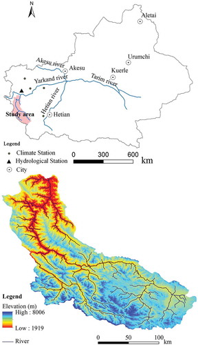
The Yarkand watershed in the Tarim River source area between latitudes 35°27'–37°44'N and longitudes 75°31'–78°24'E, covers a surface area of about 27 800 km² (Fig. 1). The Yarkand watershed, which is in the extremely arid western China, derives most of its water resources from melting snow and glaciers in the Karakoram and Kunlun mountain systems. About 64% of the discharge is from melting snow and glaciers (Alexander et al. 2008). The snowline in this area is at an altitude of about 5395 m, with the low limit at 5145 m. About 11.1% of the area is covered by glaciers. The annual average runoff is 54.62 × 10⁸ m³ (Sun et al. 2010).

Figure 1. Location of the Yarkand watershed in Xinjiang, China.

3 Data and methods

3.1 Data basis

We obtained data from European Centre for Medium-Range Weather Forecasts (ECMWF; http://www.ecmwf.int/), and daily temperature, precipitation, solar radiation and evaporation were used during the period of 1 January 1960 to 31 December 2007. Data were from ERA-40 dataset (1960–1978) and ERA-Interim dataset (1979–2007). The size of the grid cells was 0.25° × 0.25°. Streamflow and groundwater level data from Kuluk hydrological station were obtained from the Tarim River Basin Administrative Bureau (http://www.tahe.gov.cn/) during the same period. The data have been verified. A digital elevation model (DEM) was used for rectifying the precipitation and temperature in the watershed. The size of the grid cells is 100 m × 100 m. The spatial distribution of the reference stations was shown in Fig. 1.

3.2 Sensitivity analysis

Sensitivity analysis can directly show the degree to which a factor influences the runoff. If there is great change in runoff with the change of an influencing factor, the sensitivity to that factor is very high.

In order to analyse the sensitivity of runoff to climate change, a sensitivity analysis method has been introduced. The sensitivity index can be expressed as follows (Dooge et al. 1999):

(1)

where is the standard runoff and is used in comparison with a period of time; is the influencing factor (such as precipitation, evaporation and temperature) on runoff, is the difference value between the observed runoff (R) and the standard value ; is the difference value between the observed influencing factor () and the standard value .

3.3 Gaussian function

The Gaussian function, which gives the probability that an observation will fall between any two real numbers, is widely used to describe normal distribution in statistics, defining Gaussian filters in signal processing (Qian and Chen 1994), transforming Gaussian blurs in image processing (Zhang and Smart 2006), solving heat and diffusion equations and defining the Weierstrass transform in mathematics (Barcelos et al. 2005). Gaussian functions have also been applied in climate and hydrology (Nualart and Quer-Sardanyons 2012). A Gaussian function was used in the present study for analysing the response characteristics of runoff to factors to which it is sensitive.

Bi-Gaussian functions were used to improve the precision in fitting. The functions can be expressed as:

(2)

where is the sensitivity index of the ith factor; a₁, a₂, b₁, b₂, c₁ and c₂ are the Gaussian parameters; and x is the discharge (m³ s^-1).

3.4 Runoff simulation

3.4.1 MIKE 11/NAM rainfall–runoff model

The MIKE 11/NAM hydrological model has been applied to simulate the rainfall–runoff processes in the Tarim River basin (Bao et al. 2011). This model was originally developed by the Department of Hydrodynamics and Water Resources of the Technical University of Denmark. MIKE 11/NAM is a lumped and conceptual rainfall–runoff model based on physical structures and equations used together with semi-empirical ones (Madsen 2000). Being a lumped model, MIKE 11/NAM treats each catchment as a single unit. The parameters and variables represent, therefore, average values for the entire catchment. As a result, some of the model parameters can be evaluated from physical catchment data, but estimation of the final parameter must be performed by calibration against time series of hydrological observations.

The model structure (Bao et al. 2011) is shown in Fig. 2. It is an imitation of the land phase of the hydrological cycle. MIKE 11/NAM simulates the rainfall–runoff process by accounting for the water content in four different and mutually interrelated storages that represent different physical elements of the catchment. These storages are snow storage, surface storage, lower or root-zone storage and groundwater storage (Madsen 2000).

Figure 2. MIKE 11/NAM model structure (Bao et al. 2011). , water content at the wilting point in surface storage; , actual water content in surface storage; , water content at field capacity in surface storage; QOF, overland flow runoff; P, precipitation; PN, net precipitation; DL, the lower zone storage; GAFLUX, groundwater flux; Bfu, baseflow; GWPUMP, pumped groundwater; GWLBFO, maximum groundwater depth causing baseflow; S_y, specific yield for the groundwater storage; U_max, maximum water content in surface storage; L_max, maximum water content in root zone storage; CKBF, time constant for routing baseflow; CK_1,2, time constants for routing overland flow.

In addition, MIKE 11/NAM allows treatment of man-made interventions in the hydrological cycle such as irrigation and groundwater pumping. Based on the meteorological input data, MIKE 11/NAM produces catchment runoff as well as information about other elements of the land phase of the hydrological cycle, such as the temporal variation of the evaporation, soil moisture content, groundwater recharge, and groundwater levels. The resulting catchment runoff is split conceptually into overland flow, interflow and baseflow.

The MIKE11/NAM model needs (a) model parameters, (b) initial conditions, (c) meteorological data (precipitation, potential evaporation, temperature and radiation), and (d) streamflow data for the model calibration and validation. The model setup could be referred to the reference manual (DHI 2009).

3.4.2 Model uncertainty estimation

The coefficient of efficiency is generally used to evaluate model performance (Nash and Sutcliffe 1970, McMichael et al. 2006). It can be expressed as:

(3)

where O and are the observed discharge and the mean observed discharge, respectively, and P is the predicted discharge. If the predicted values are equal to the mean observed discharge, E = 0. When all the predicted values equal to their corresponding observations, then E = 1.

To evaluate the difference between the predicted discharge and the observed discharge, relative error is frequently used (Kokkonen et al. 2001):

(4)

The closer to 0 is, the higher the accuracy is.

3.5 Pearson product–moment correlation analysis

Statistical parameters can reflect the basic characteristics of a random phenomenon. Pearson product–moment correlation analysis is one of the most popular classical statistical methods (Cristescu et al. 2012). It is often used to express the closeness of the relationship between two or more variables. Statistical parameters and Pearson product–moment correlation analysis are all widely applied in hydrology and water resources management (Ouarda et al. 2001, Tsakiris et al. 2011). They were introduced to analyse the relationship between runoff and meteorology in order to identify the main influencing factors. The correlation coefficients between monthly average runoff and monthly average precipitation, average temperature, average evaporation, average sunshine hours and average wind speed were calculated.

First, the meteorological factors with close relationship between discharge and dissipation such as precipitation, average temperature, evaporation, radiation and wind speed (Hodgkins 2001), were selected to construct the monthly data series from 1960 to 2007. The contemporaneous runoff series were also constructed. Then the fluctuating part of each series about the average was calculated. Finally, the statistical parameters, including average, coefficient of variation, coefficient of skewness and correlation coefficients (Kravtsov et al. 2005), were analysed. Coefficient of variation is a normalized measurement of dispersion of a probability distribution, and the coefficient of skewness is a measurement of the asymmetry of the probability distribution of a real-valued random variable (Bendel et al. 1989).

3.6 Temperature and precipitation revision

Temperature and precipitation data are required to be corrected for reducing errors caused by low resolution and location deviation. Empirical formulas, calculated from the relationship between elevation and climate data, were used to correct data in this paper. First, the elevation of each grid cell within the reference stations area was calculated with DEM. Then the temperature (Yang et al. 2007) and precipitation (Ji and Chen 2012) in the area would be calculated according to the empirical formulas. If the relative error between the calculated and observed values was less than 10%, it meant that the data could be used. Otherwise the data was revised. All work was performed using the spatial analysis model in ARCGIS 10.1.

3.7 Calibration of parameters

All the discharges used for calibration were measured during 1990 and 1995. Temperature, precipitation, solar radiation, evaporation and discharge were daily average values. The two periods which were assumed to have the minimum and maximum effects of the climate on the runoff were chosen for calibration. Calibration to measured discharge was performed through an iterative process of changing water content, overland flow runoff coefficient and time constant.

The main parameter setting used in the modelling system was listed in Table 1. The values listed are the final calibrated values of parameters.

Table 1. MIKE11/NAM model parameters.

Parameter	Umax	Lmax	CQOF	CKIF	CK1,2
Value	14.6	82.6	0.743	17	14.4
Parameter	TOF	TIF	TG	CKBF
Value	0.96	0.988	0.189	1241

Note: Umax, maximum water content in surface storage; Lmax, maximum water content in root zone storage; CQOF, overland flow runoff coefficient; CKIF, time constant for inter flow; CK_1,2, time constants for routing overland flow; TOF, root zone threshold value for overland flow; TOF, TIF, TG, root zone threshold value for overland flow, inter flow, groundwater recharge, respectively; CKBF, time constant for routing base flow.

4 Results and discussion

4.1 Fluctuation characteristics and correlation analysis between runoff and climate factors

Based on the above correlation analysis method, the climatic variables were correlated with monthly average runoff, and some statistical parameters were calculated. The results are shown in Table 2.

Table 2. The statistical characteristics of runoff and climate factors (n = 576).

Item	Monthly average runoff (×10^8 m^3)	Monthly average precipitation (mm)	Monthly average temperature (°C)	Monthly average evaporation (mm)	Monthly average sunshine hours (h per month)	Monthly average wind speed (m s^-1)
Average	4.205	29.125	−5.229	25.069	242.189	2.353
Coefficient of variation	1.308	1.399	0.274	0.581	0.044	0.160
Coefficient of skewness	1.918	1.995	−0.172	0.197	−0.204	−0.608
Correlation coefficient with monthly average runoff		0.4521**	0.4604**	0.7261**	0.0453	0.1102

**Believable probabilities of data are over 95%.

The results show that the Yarkand watershed is characterized by a typical continental climate with little precipitation, low temperature, intensive evaporation, rich sunlight and low wind speed. The coefficients of variation of runoff and precipitation are larger than the others. Monthly average sunshine hours and wind speed are very small. The reason for this is that the Yarkand watershed is surrounded by the Kunlun Mountains in the south, Tianshan Mountains in the north and Pamirs plateau in the west. Mountains block the input of vapor in the atmosphere so that most of the precipitation falls on the windward side. The runoff and precipitation have positively skewed distributions, whilst the monthly average temperature, sunshine hours and wind speed have negatively skewed distributions. This is consistent with the coefficients of variation. Correlation analysis shows that there is a positive correlation between discharge and the meteorological factors. Only the confidence interval of precipitation, temperature and evaporation are over 95%. The correlation coefficient of evaporation is the largest one, and is followed by the average temperature. Thus, the meteorological factors with significant effect on runoff are evaporation, temperature and precipitation.

4.2 Time-varying response characteristics of sensitivity indexes

Following the correlation analysis, the factors that have the most significant effect on runoff, evaporation, temperature and precipitation, were chosen for further analysis.

4.2.1 Time-varying characteristics of sensitivity indexes

The daily sensitivity indexes of precipitation, evaporation and temperature from 1960 to 2007 were calculated using equation (1). The standard runoff () adopted the daily averages of all 48 years. The monthly (Fig. 3) and annual (Fig. 4) sensitivity indexes were based on the daily values.

Figure 3. Annual variation of sensitivity indexes in the Yarkand watershed.

Figure 4. Monthly variation of sensitivity indexes in the Yarkand watershed.

Figure 3 shows that the sensitivity indexes changed annually. All of them had a similar trend. The sensitivity index of precipitation, 2.75, is the largest in synchronization. The sensitivity indexes of temperature and evaporation rank the second and the third, 1.30 and 1.05, respectively. The maximum values of all the three indexes occurred in 1995, being 3.73, 1.76 and 2.54 for precipitation, temperature and evaporation, respectively. The minimum values, 2.22 for precipitation, 0.98 for temperature and 0.41 for evaporation, were observed in 1990. This shows that precipitation is the most sensitive factor among these factors to the runoff in the study area. The large annual variation of sensitivity indexes suggests there is a close relationship between the sensitive factors and external factors.

Figure 4 shows the monthly sensitivity indexes, which showed double peaks. The size order was similar to that of the annual variation: precipitation > temperature > evaporation. The main and the secondary peak values appeared in June and September, and the valley values appeared in August. The consistency of sensitivity shows the close relationship among these factors. June and September, when peak values appear, are the flooding period and the dry period, respectively. We can take measures according to the sensitivity change based on the different sensitive factors.

4.2.2 Distribution characteristics of sensitivity indexes with discharge

To describe fully the statistical regularity of random variables, the distribution function is always used. A review of literature shows that precipitation and runoff can be expressed by distribution functions but there are some differences in different areas. In order to find the differences and their regularities with runoff, a method of parametrization of Gaussian functions was adopted in the present study. Gaussian functions were always used for curve fitting. Jonsson and Eklundh (2002) simulated the entire growing season of plants and determined the time of the beginning and end of the growing season using such function. Asymmetrical Gaussian functions were used instead of common Gaussian functions to analyse the skewed distributions. First, the data points were fit around the extreme value using partial Gaussian functions. Then the fitted contiguous functions were spliced for the global functions.

First, the daily series of sensitivity indexes of precipitation, temperature and evaporation were calculated for a period of 48 years. Then all series were sorted based on daily discharge, and the sensitivity indexes of each factor affecting discharge were fit using bi-Gaussian functions. The fitting curves are shown in Fig. 5.

Figure 5. Fitting curves of sensitivity index with discharge.

The fitting equations are as follows at the 95% confidence level:

(5)

(6)

(7)

: sensitivity index of temperature, : sensitivity index of evaporation, : sensitivity index of precipitation.

The fitting errors, sum of squares for error (SSE), determination coefficients (R²) and root mean square error (RMSE) were obtained by further analysis (Table 3).

Table 3. The statistics of the fitting errors.

Title	SSE (sum of squaresfor error)	R^2 (determinationcoefficients)	RMSE (root meansquare error)
Temperature	107.7	0.9469	0.6062
Evaporation	145.5	0.9075	0.7046
Rain	758.2	0.7375	1.62

The fitting result shows that bi-Gaussian functions can describe the distribution between sensitivity index and runoff. Parameter a₁ in equation (2) represents the peak value. It is 34.74, 16.64 and 21.37 for precipitation, temperature and evaporation, respectively. This indicates that precipitation has more influence on runoff than temperature and evaporation under extreme conditions. Parameter b₁ represents the location of the axis of symmetry on the x-axis. The values of three factors are not significant. But all median discharges are about 165 m³ s^-1. Parameter c₁ is the steepness of the curve. The smaller c1 is, the steeper the curve is. Here, it represents the sensitive range for runoff. The fitting results indicate that the influencing range of climate factors increase from the smallest to the largest in the order of evaporation, temperature and precipitation.

4.3 The sensitivity simulation of runoff with the governing climate factors

4.3.1 Model calibration, testing, and estimation of uncertainty

According to the above analysis, the peak value and valley value of sensitivity indexes appeared in 1990 and 1995, respectively, so their runoff processes were chosen for the model calibration and testing. This work is the foundation for simulation of runoff sensitivity to climate change.

Parameter sets (see Table 1 for the main initial parameters) were used to conduct the Yarkand simulation for a calibration period from January 1 to 31 December 1990 (Fig. 6). The value of E is 0.8632 (Table 4) for the runoff at Kuluk. The threshold value of E applied in our application of MIKE 11/NAM agrees with those reported by Andersen et al. (2001) and McMichael et al. (2006), who found good model runs for E ≥ 0.65. The results indicate that the model is acceptable for conducting a simulation of the Yarkand watershed.

Table 4. Estimate of uncertainty at Kuluk.

Title	E calibration	Dv
Calibration period (January 1–December 31 1990)	0.8632	−0.22
Test period (January 1–December 31 1995)	0.8321	4.33

Figure 6. Observed and simulated streamflow in the calibration period (1990).

We calculated prediction errors for daily data over the test period (1 January–31 December 1995) (Fig. 7). Approximately 85% of the observed runoff values fell within the 5% and 95% uncertainty bounds based on regression versus observed values. The accuracy of the model predictions is considered to be acceptable (McMichael et al. 2006).

Figure 7. Observed and simulated streamflow in the test period (1995).

4.3.2 Simulation of runoff sensitivity to climate change

To analyse the impact of key meteorological factors on runoff, several schemes were constructed for modeling.

4.3.2.1. Design of simulation scheme

To contrast the differences in the impact of climate change on runoff under different sensitivity backgrounds, the meteorological data in 1990 and 1995 representing the most sensitive and the least sensitive background values, respectively, were selected as the standard values for simulation. The temperature ranges from −2°C to 2°C, and precipitation ranges from −20% to +20% (Sun et al. 2010) in the Yarkand watershed. Based on the standard background values, we assumed: −2°C, 0°C and 2°C change of the temperature; −20%, 0 and +20% change of the precipitation; −20%, 0 and +20% change of the evaporation. Then 27 sets of simulating meteorological data were obtained. On the other hand, three climate seniors with respect to the baseline period 1961 to 1990 were chosen, based on the Fourth Assessment Report (AR4) Atmosphere-Ocean General Circulation Models (AOGCMs) by IPCC (http://www.ipcc.ch/publications_and_data/ar4/wg2/en/ch10s10-3.html). The combination schemes are shown in Table 5.

Table 5. Assumed climate change schemes.

Scenarios	ΔT (°C)	ΔP (%)	ΔE (%)
1	−2.0	−20	−20%
2	−2.0	−20	0
3	−2.0	−20	+20%
4	−2.0	0	−20%
5	−2.0	0	0
6	−2.0	0	+20%
7	−2.0	+20	−20%
8	−2.0	+20	0
9	−2.0	+20	+20%
10	0	−20	−20%
11	0	−20	0
12	0	−20	+20%
13	0	0	−20%
14	0	0	0
15	0	0	+20%
16	0	+20	−20%
17	0	+20	0
18	0	+20	+20%
19	+2.0	−20	−20%
20	+2.0	−20	0
21	+2.0	−20	+20%
22	+2.0	0	−20%
23	+2.0	0	0
24	+2.0	0	+20%
25	+2.0	+20	−20%
26	+2.0	+20	0
27	+2.0	+20	+20%
28 (IPCC: 2010–2039)	1.68	0.88	–
29 (IPCC: 2040–2069)	3.38	0.25	–
30 (IPCC: 2070–2099)	5.14	−3.00	–

4.3.2.2 Impact of fluctuating meteorological factors on runoff

The runoff in the 30 sets of scenarios was simulated. The annual average and monthly average runoff were analysed based on the simulation results (Figs 8 and 9). In order to display the result clearly, the monthly average runoff and change rate under all scenarios were calculated (Fig. 9).

Figure 8. Comparison of the annual average runoff based on different simulated background values of sensitivity.

Figure 9. Simulated monthly average runoff in the different scenarios (a) Average monthly change rate of 27 assumed climate seniors; (b) average monthly change rate of IPCC climate seniors based on AR4.

Figure 8 shows that the annual average runoff would have a decreasing trend if the meteorological data of 1990 were adopted as the reference standard: 74.1% of the scenarios led to significant decreases. The range of the decrease in runoff was 4.26%. The maximum appeared in the 12th scenario, with a 20% decrease of precipitation and a 20% increase of evaporation. The decrement of runoff reached 14.57%. On the other hand, there would be an increasing trend if the reference standard adopted were the meteorological data of 1995: 85.2% of the scenarios led to significantly increased runoff. The range of the increase in runoff was 2.61%. The maximum appeared in the 21st scenario, with a 2°C increase in temperature, a 20% decrease in precipitation and a 20% increase in evaporation. The increment of runoff reached 8.80%. Further analysis indicates that the influences of temperature, precipitation and evaporation on runoff are different. There is a positive correlation between runoff and evaporation whereas the correlation between temperature and precipitation can be either positive or negative. On the whole, under the maximum sensitivity scenario, the largest fluctuation influences among the meteorological factors are those of evaporation, and the smallest are those of temperature. Under the minimum sensitivity scenario, the largest is that of precipitation, and the smallest is that of evaporation.

Figure 9 shows the monthly average fluctuation of runoff under all scenarios. There is a decreasing trend from February to June and an increasing trend in the other months. Among the changes, the increment of runoff reached 85.27% in May. The annual average runoff has a slight increasing trend. The discharge change mainly distributed in the summer (April to June) and winter (December to February).

The analysis as a whole shows that the impact of climate on runoff is different under different scenarios. Differences in the initial meteorological conditions can also lead to big differences in runoff. If the initial sensitivity of runoff to climate were strong, climate change would cause annual runoff to increase. Conversely, if the sensitivity were weak, climate change would cause annual runoff to decrease. The flow variation in autumn and winter would be greater than that in spring and summer. The factor with the greatest influence on runoff is the evaporation. However, the influences of temperature and precipitation are not so stable. In a certain range, precipitation change may cause great fluctuations of runoff while temperature change may not result in great runoff fluctuation.

5 Conclusions

Sensitivity analysis has been applied extensively in engineering, economics, medicine, meteorology and hydrology. In the present study, this method was used to analyse the impact of climate on runoff. It was demonstrated that sensitivity can reflect the response relationship between runoff and climate change in the study area. Significant correlations were found between runoff and precipitation, evaporation and temperature. The sensitivity of runoff to these climate factors changed with time and fluctuated synchronously. The runoff is most sensitive to precipitation and least sensitive to evaporation.

All the sensitivities could be fit with Gaussian distributions. Bi-Gaussian functions satisfactorily describe the sensitivity of runoff to the various factors. All regression determination coefficients were above 0.7. The fitting results show that the largest influence of climate on runoff is centered on the axis of symmetry with a range of ±100 m³ s^-1. When the runoff is out of this range, the influence becomes weak.

The MIKE 11/NAM model was applied extensively, and the performance of the model was assessed using the coefficient of efficiency E (Nash and Sutcliffe 1970, McMichael et al. 2006). This coefficient was greater than 0.8, and approximately 85% of the observed runoff values were within the 5% and 95% uncertainty bounds of the regression of simulated versus observed runoff. This result shows that the NAM model is acceptable for the simulation of precipitation runoff in the study area.

On the basis of modelling the impact of 30 sets of schemes, it was found that change of annual runoff is related to the initial climate condition. The annual runoff has a decreasing trend if it has a weak sensitivity to the initial climate condition; conversely, it has an increasing trend if the sensitivity is strong. The runoff decreases linearly with increasing evaporation. There are only positive relationships between runoff and temperature. In addition, the impact of climate change on runoff is larger in summer and winter than in spring and autumn.

This study describes an efficient method for analysing the impact of climate on runoff. Estimation of the spatial-temporal influence of climate on runoff could provide insight for water resource development in arid areas.

Acknowledgements

The authors would like to thank the anonymous reviewers for suggesting improvements to the manuscript.

Disclosure statement

No potential conflict of interest was reported by the author(s).

Additional information

Funding

This work was supported by the National 973 Key Project of China (2010CB951004), the Natural Foundation of China (41161008), National Key Technology Support Program of China (2012BAH27B03), and the natural science and Technological Innovation Project of Shihezi University (2011ZRKXTD-0304).

References

- Alexander, N.V., et al., 2008. Assessments and decreasing of risks and damages from outbursts of Tien Shan high mountains lakes. In: B.J. Merkel and H.B. Andrea, eds. Uranium: Mining and Hydrogeology. Berlin: Springer Verlag, 819–826.
- Andersen, J., Refsgaard, J.C., and Jensen, K.H., 2001. Distributed hydrological modelling of the Senegal River Basin — model construction and validation. Journal of Hydrology, 247, 200–214. doi:10.1016/S0022-1694(01)00384-5
- Bao, A.-M., et al., 2011. The effect of estimating areal rainfall using self-similarity topography method on the simulation accuracy of runoff prediction. Hydrological Processes, 25 (22), 3506–3512. doi:10.1002/hyp.8078
- Barcelos, C.A.Z., et al., 2005. Edge detection and noise removal by use of a partial differential equation with automatic selection of parameters. Computational & Applied Mathematics, 24 (1), 131–150. doi:10.1590/S0101-82052005000100008
- Bendel, R.B., et al., 1989. Comparison of skewness coefficient, coefficient of variation, and Gini coefficient as inequality measures within populations. Oecologia, 78, 394–400. doi:10.1007/BF00379115
- Canham, C.D. and Thomas, R.Q., 2010. Frequency, not relative abundance, of temperate tree species varies along climate gradients in eastern North America. Ecology, 91, 3433–3440. doi:10.1890/10-0312.1
- Chen, Y.-N., et al., 2007. Effects of climate change on water resources in Tarim River Basin, Northwest China. Journal of Environmental Sciences, 19 (4), 488–493. doi:10.1016/S1001-0742(07)60082-5
- Chiew, F.H.S., 2006. Estimation of rainfall elasticity of streamflow in Australia. Hydrological Sciences Journal, 51 (4), 613–625. doi:10.1623/hysj.51.4.613
- Cristescu, C.P., et al., 2012. Parameter motivated mutual correlation analysis: application to the study of currency exchange rates based on intermittency parameter and Hurst exponent. Physica A: Statistical Mechanics and its Applications, 391 (8), 2623–2635. doi:10.1016/j.physa.2011.12.006
- Delbari, M., Afrasiab, P., and Loiskandl, W., 2009. Using sequential Gaussian simulation to assess the field-scale spatial uncertainty of soil water content. Catena, 79 (2), 163–169. doi:10.1016/j.catena.2009.08.001
- DHI, 2009. MIKE 11: A modeling system for rivers and channels. Reference manual. Denmark: Danish Hydraulic Institute.
- Donohue, R.J., Roderick, M.L., and McVicar, T.R., 2011. Assessing the differences in sensitivities of runoff to changes in climatic conditions across a large basin. Journal of Hydrology, 406 (3–4), 234–244. doi:10.1016/j.jhydrol.2011.07.003
- Dooge, J.C.I., Bruen, M., and Parmentier, B., 1999. A simple model for estimating the sensitivity of runoff to long-term changes in precipitation without a change in vegetation. Advances in Water Resources, 23 (2), 153–163. doi:10.1016/S0309-1708(99)00019-6
- Forchini, G., 2000. The density of the sufficient statistics for a Gaussian AR(1) model in terms of generalized functions. Statistics & Probability Letters, 50 (3), 237–243. doi:10.1016/S0167-7152(00)00111-5
- Fu, G.B., Charles, S.P., and Chiew, F.H.S., 2007. A two-parameter climate elasticity of streamflow index to assess climate change effects on annual streamflow. Water Resources Reserach, 43 (11), W11419. doi:10.1029/2007WR005890.
- Hagen, N. and Dereniak, E.L., 2008. Gaussian profile estimation in two dimensions. Applications Optical, 47 (36), 6842–6851. doi:10.1364/AO.47.006842
- Havnø, K., Madsen, M.N., and Dørge, J., 1995. MIKE 11-a generalized river modelling package. In: V.P. Singh, Ed. Computer Models of Watershed Hydrology. Littleton, CO: Water Resources Publications, 733–782.
- Hodgkins, R., 2001. Seasonal evolution of meltwater generation, storage and discharge at a non-temperate glacier in Svalbard. Hydrological Processes, 15 (3), 441–460. doi:10.1002/hyp.160
- Huang, X., et al., 2010. Study on change in value of ecosystem service function of Tarim River. Acta Ecologica Sinica, 30 (2), 67–75. doi:10.1016/j.chnaes.2010.03.004
- Ji, X. and Chen, Y., 2012. Characterizing spatial patterns of precipitation based on corrected TRMM3B43 data over the mid Tianshan Mountains of China. Journal of Mountain Science, 9 (5), 628–645. doi:10.1007/s11629-012-2283-z
- Jones, R.N., et al., 2006. Estimating the sensitivity of mean annual runoff to climate change using selected hydrological models. Advances in Water Resources, 29 (10), 1419–1429. doi:10.1016/j.advwatres.2005.11.001
- Jonsson, P. and Eklundh, L., 2002. Seasonality extraction by function fitting to time-series of satellite sensor data. IEEE Transactions on Geoscience and Remote Sensing, 40 (8), 1824–1832. doi:10.1109/TGRS.2002.802519
- Kapeller, S., et al., 2012. Intraspecific variation in climate response of Norway spruce in the eastern Alpine range: selecting appropriate provenances for future climate. Forest Ecology and Management, 271, 46–57. doi:10.1016/j.foreco.2012.01.039
- Khaleel, R., Reddy, K.R., and Overcash, M.R., 1980. Transport of potential pollutants in runoff water from land areas receiving animal wastes: A review. Water Research, 14 (5), 421–436. doi:10.1016/0043-1354(80)90206-7
- Kling, H., Fuchs, M., and Paulin, M., 2012. Runoff conditions in the upper Danube basin under an ensemble of climate change scenarios. Journal of Hydrology, 424-425 (0), 264–277. doi:10.1016/j.jhydrol.2012.01.011
- Kokkonen, T., Koivusalo, H., and Karvonen, T., 2001. A semi-distributed approach to rainfall–runoff modelling –a case study in a snow affected catchment. Environmental Modelling & Software, 16 (5), 481–493. doi:10.1016/S1364-8152(01)00028-7
- Kravtsov, Y., et al., 2005. Estimating statistical parameters of an elastic random medium from traveltime fluctuations of refracted waves. Waves in Random and Complex Media, 15, 43–60. doi:10.1080/17455030500052478
- L’vovich, M.I., 1979. World water resources and their future. Washington, DC: American Geophysical Union.
- Liu, H.-L., et al., 2007. Investigation of groundwater response to overland flow and topography using a coupled MIKE SHE/MIKE 11 modeling system for an arid watershed. Journal of Hydrology, 347 (3–4), 448–459. doi:10.1016/j.jhydrol.2007.09.053
- Madsen, H., 2000. Automatic calibration of a conceptual rainfall–runoff model using multiple objectives. Journal of Hydrology, 235 (3–4), 276–288. doi:10.1016/S0022-1694(00)00279-1
- Marian, P. and Marian, T.A., 1996. Photon number and counting statistics for a field with Gaussian characteristic function. Annals of Physics, 245 (1), 98–112. doi:10.1006/aphy.1996.0004
- McMichael, C.E., Hope, A.S., and Loaiciga, H.A., 2006. Distributed hydrological modelling in California semi-arid shrublands: MIKE SHE model calibration and uncertainty estimation. Journal of Hydrology, 317 (3–4), 307–324. doi:10.1016/j.jhydrol.2005.05.023
- Milliken, J.G., 1989. Water resources management in arid climates. Desalination, 72 (1–2), 173–184. doi:10.1016/0011-9164(89)80034-7
- Nash, J.E. and Sutcliffe, J.V., 1970. River flow forecasting through conceptual models part I — A discussion of principles. Journal of Hydrology, 10, 282–290. doi:10.1016/0022-1694(70)90255-6
- Nielsen, S.A. and Hansen, E., 1973. Numerical simulation of the rainfall runoff process on a daily basis. Nordic Hydrology, 4, 171–190.
- Nualart, E. and Quer-Sardanyons, L., 2012. Gaussian estimates for the density of the non-linear stochastic heat equation in any space dimension. Stochastic Processes and Their Applications, 122 (1), 418–447. doi:10.1016/j.spa.2011.08.013
- Ouarda, T.B.M.J., et al., 2001. Regional flood frequency estimation with canonical correlation analysis. Journal of Hydrology, 254 (1–4), 157–173. doi:10.1016/S0022-1694(01)00488-7
- Qian, S. and Chen, D., 1994. Signal representation using adaptive normalized Gaussian functions. Signal Processing, 36 (1), 1–11. doi:10.1016/0165-1684(94)90174-0
- Sankarasubramanian, A. and Vogel, R.M., 2003. Hydroclimatology of the continental United States. Geophys. Res. Lett., 30 (7), 1–4. doi:10.1029/2002GL015937
- Sankarasubramanian, A., Vogel, R.M., and Limbrunner, J.F., 2001. Climate elasticity of streamflow in the United States. Water Resour. Res., 37 (6), 1771–1781. doi:10.1029/2000WR900330
- Schaake, J.C., 1990. From climate to flow. In: P.E. Waggoner, Ed. Climate Change and US Water Resources. New York: John Wiley, 117–206.
- Singha, R., et al., 2014. Impact of water management interventions on hydrology and ecosystem services in Garhkundar-Dabar watershed of Bundelkhand region, Central India. Journal of Hydrology, 509 (13), 132–149. doi:10.1016/j.jhydrol.2013.11.030
- Sun, G.L., et al., 2010. The response of glacial lake outburst floods to climate change in the Yarkant River, Xinjiang. Journal of Glaciology and Geocryology, 32 (3), 580–586.
- Tsakiris, G., Nalbantis, I., and Cavadias, G., 2011. Regionalization of low flows based on Canonical Correlation Analysis. Advances in Water Resources, 34 (7), 865–872. doi:10.1016/j.advwatres.2011.04.007
- Weissler, F.B., 1981. Existence and non-existence of global solutions for a semilinear heat equation. Israel Journal of Mathematics, 38 (1–2), 29–40. doi:10.1007/BF02761845
- Xu, H.-L., Ye, M., and Li, J.-M., 2007. Changes in groundwater levels and the response of natural vegetation to transfer of water to the lower reaches of the Tarim River. Journal of Environmental Sciences, 19 (10), 1199–1207. doi:10.1016/S1001-0742(07)60196-X
- Yang, X., et al., 2007. Terrain revised model for air temperature in mountainous area based on DEMs. Journal of Geographical Sciences, 17 (4), 399–408. doi:10.1007/s11442-007-0399-9
- Zhang, M. and Smart, W., 2006. Using Gaussian distribution to construct fitness functions in genetic programming for multiclass object classification. Pattern Recognition Letters, 27 (11), 1266–1274. doi:10.1016/j.patrec.2005.07.024