Multiple linear regression, multi-layer perceptron network and adaptive neuro-fuzzy inference system for forecasting precipitation based on large-scale climate signals

ABSTRACT

Nowadays, mathematical models are widely used to predict climate processes, but little has been done to compare the models. In this study, multiple linear regression (MLR), multi-layer perceptron (MLP) network and adaptive neuro-fuzzy inference system (ANFIS) models were compared for precipitation forecasting. The large-scale climate signals were considered as inputs to the applied models. After selecting the most effective climate indices, the effects of large-scale climate signals on the seasonal standardized precipitation index (SPI) of the Maharlu-Bakhtaran catchment, Iran, simultaneously and with a delay, was analysed using a cross-correlation function. Hence, the SPI time series was forecasted up to four time intervals using MLR, MLP and ANFIS. The results showed that most of the indices were significant with SPI of different lag times. Comparison of the SPI forecast results by MLR, MLP and ANFIS models showed better performance for the MLP network than the other two models (RMSE = 0.86, MAE = 0.74 for the first step ahead of SPI forecasting).

Editor D. Koutsoyiannis; Associate editor F. Pappenberger

KEYWORDS:

• climate signals
• standardized precipitation index
• multiple linear regression
• adaptive neuro-fuzzy inference system
• multi-layer perceptron network

1 Introduction

Precipitation forecasting has always been one of the most important issues in the hydrological cycle and it is essential in water resource development, planning and management of droughts. In Iran, like many other arid parts of the world, there are regions that have arid climate and drought events. Therefore, it is necessary to give more attention to sparse precipitation. Forecasting of hydrometeorological parameters using global climate indices has become a necessity for water resources management (Abtew et al. 2009). In recent decades, many researchers have studied the impact of these signals on hydroclimatic data in different areas (Wallace 2000, Turkes and Elart 2003, Seleshi and Zanke 2004, Grantz et al. 2005, Cañón et al. 2007, Kumar et al. 2007, Abtew et al. 2009, Kalra and Ahmad 2009, Fallah-Ghalhary et al. 2010, Gámiz-Fortis et al. 2010, Berg et al. 2013, Kalra et al. 2013).

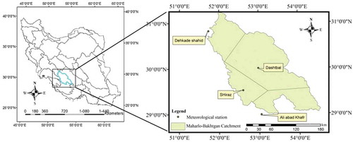
Figure 1. Map of the Maharlu-Bakhtegan catchment and the gauging stations, southwest of Iran.

Trafalis et al. (2002) used linear regression models and feedforward artificial neural networks (ANNs) for precipitation forecasting and the result showed that the performance of ANNs was more accurate than the linear regression. Valverde Ramírez et al. (2005) demonstrated that the ANN was superior to linear regression in rainfall forecasting. Chattopadhyay (2007) also indicated that the feedforward ANN model has lower errors than multiple linear regression (MLR) in predicting average summer monsoon rainfall over India. Dahamsheh and Aksoy (2009) suggested that the ANNs were slightly better than MLR in forecasting the monthly total precipitation of arid regions. Azadi and Sepaskhah (2012) concluded that neural networks did not significantly increase prediction accuracy compared with the multiple regression model. Dastorani et al. (2010) indicated that the potential of ANN for dryland precipitation forecasting is almost the same as that of adaptive neuro-fuzzy inference system (ANFIS) model. Some researchers, such as Fallah-Ghalhary et al. (2010) for rainfall forecasting using large-scale synoptic patterns, El-Shafie et al. (2011) in rainfall forecasting, Sanikhani and Kisi (2012) in the estimation of monthly streamflows, and Jeong et al. (2012) for monthly precipitation forecasting using climatological and hydrological monthly data, have suggested that the ANFIS model can predict precipitation with reasonable accuracy. The main objective of this study was to assess the performance of MLR, multi-layer perceptron (MLP) networks and ANFIS to forecast seasonal precipitation based on different large-scale climate signals.

2 Methodology

2.1 Study area and dataset

The Maharlu-Bakhtegan catchment, having an area of 31 000 km², is located at 29°00'–31°14'N and 51°42'–54°31'W (Fig. 1), in the southwest of Iran. This catchment is one of the most fertile agricultural areas of Iran. It includes the three sub-domains of Kaftar, Bakhtegan and Maharlu lakes. The Kor is the most important river in the region. The amount of precipitation in this catchment is variable, between 200 mm in the southeast and 700 mm in the northwest, and mainly occurs in winter and spring. The maximum elevation of the Maharlou-Bakhtegan catchment is in the northwest (3941 m a.s.l.) in the Sefid mountains, while the minimum elevation is in the southwest (1455 m a.s.l.) at Maharlou Lake.

Since water resources management is necessary in arid regions such as Iran, the water resources managers are interested in long-term forecasts. However, precipitation data with a short time interval, such as daily precipitation, have been mostly used in limited studies (Kim et al. 2008). So, this study has focused on the seasonal standardized precipitation index (SPI) and climate signals. Precipitation data (from January 1967 to December 2009) were collected from four meteorological stations, Shiraz, Dashtbal, Ali Abad and Dehkadeh Shahid (Fig. 1). Then, the seasonal SPI was calculated. The average annual precipitation over the catchment is 360 mm. Meanwhile, climate index data were obtained from the US National Oceanic and Atmospheric Administration website (http://www.esrl.noaa.gov/psd/data/climateindices/list/).

2.2 Principal component analysis (PCA)

The PCA method is an unsupervised nonparametric multivariate statistical technique (Faria et al. 2007, Ringnér 2008) that is applied to reduce the dimensionality of a dataset by transforming it into a new set of variables (Jolliffe et al. 1980). In the PCA method, the variables are placed in components, so that the percentage of the variance will decrease from one variable to the next. Therefore, variables included in the first component are the most important. In the PCA method, the number of principal components is less than or equal to the number of original variables and is sensitive to the relative range of the original variables. To produce a reliable result in PCA, large enough sample sizes are required. To detect sampling adequacy the Kaiser-Meyer-Olkin (KMO) (Kaiser 1970, 1974) measure was used, which varies between 0 and 1, where values closer to 1 are better; a value of 0.6 is a suggested as a minimum. In this study, the most effective large-scale climate signals were determined using the PCA method.

2.3 Cross-correlation

Cross-correlation analysis is a standard method for determining the degree of correlation between two variables. Suppose that we have two series x_i and y_i, where i = 0, 1, 2, …, N − 1, and and are the average amounts of the x_i and y_i time intervals. The cross-correlation (CC) at delay d is defined as:

(1)

If this equation is clarified for all time delays, d = 0, ±1, ±2, …, N − 1, then we have the maximum correlation in one step of the delays. By considering the condition in this equation, these points were not in the focus i < 0 and i ≥ N, so the value of the cross-correlation coefficient will always be. In this study we used cross-correlation to determine the correlation between the most effective climate signals and SPI time series at various time lags. Karabork et al. (2005) applied cross-correlation analyses to demonstrate the teleconnections between climatic variables and climatic indices (North Atlantic Oscillation, NAO, and Southern Oscillation, SO).

2.4 Multiple linear regression (MLR)

The MLR approach predicts values of a dependent variable Y when independent variables (X₁, X₂, …, X_n) are given (Quraishi and Mouazen 2013). In this study, stepwise MLR was used to predict SPI time series using significant climate indices in the cross-correlation. The MLR equation takes the following form:

(2)

where y is the dependent variable, a is the constant value or intercept of the regression line and Y axis, b_i is the amount the response variable Y changes by the independent variables X_i: X₁, X₂, …, X_n. According to this approach, 80% of the data were considered in making the regression equation. Then the variance inflation factor (VIF) was calculated for determining the multicollinearities, as follows:

(3)

where is the multiple determination coefficient obtained from X_i regression on the K − 1 independent variables residual. If VIF = 1, no intercorrelation exists between the independent variables; if VIF stays within the range 1–5, the corresponding model is acceptable; if VIF > 10, the corresponding model is unstable (Famini et al. 1992). Finally, the regression equation was tested with the remaining 20% of the data.

2.5 Adaptive neuro-fuzzy inference system (ANFIS)

The ANFIS model is a multi-layer feedforward network using ANN learning algorithms and fuzzy reasoning to characterize an input space to an output space (Firat and Güngör 2007).

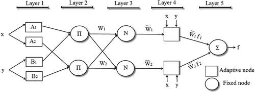
This system was introduced by Jang (1993) and the main point in designing a neuro-fuzzy system is the selection of a suitable fuzzy inference system (FIS). The basic structure of ANFIS is based on the Sugeno method of FIS, proposed by Takagi and Sugeno (1985). For the first-order Sugeno FIS, a set of rules consisting of two if–then rules is available:

• Rule 1: If x is equal to A₁ and y is equal to B₁, then p₁x + q₁y + r₁ = f₁

• Rule 2: If x is equal to A₂ and y is equal to B₂, then p₂x + q₂y + r₂ = f₂

In these rules, A₁, A₂, B₁ and B₂ are membership functions for x and y inputs and p₁, q₁, r₁, p₂, q₂ and r₂ are output function parameters (Kisi and Shiri 2011).

In the ANFIS model, grid partition (Jang and Sun 1995) and subtractive fuzzy clustering (Chiu 1994) are the most widespread methods that have been proposed to establish the rules. Grid partition is a suitable method for a few input variables, but when there are many input variables we need to consider membership functions for each of them; we cannot use this method because the number of rules will be prohibitive. Calculation of the parameters of the grid partition method with many input variables is very difficult. Therefore, in the present study, subtractive fuzzy clustering was used to establish the rule-based relationship between the input and output variables (Farokhnia et al. 2011). In this study, a hybrid learning algorithm was used for estimating membership function parameters. The hybrid optimization method is a combination of least-squares and the back-propagation gradient descent method (Rumelhart et al. 1986). The number of membership functions was determined by trial and error, and a Gaussian function was used as the optimal membership function (based on trial and error) whose output can be calculated as follows:

(4)

where {c_i and σ_i} are set parameters and the maximum will be 1 and minimum zero (Jang 1993). Figure 2 shows the structure of the ANFIS model, where x and y are ANFIS model inputs; A₁, A₂, B₁ and B₂ are fuzzy subsets; Π is layer 2 fixed nodes; w_i is the weight of a given fuzzy rule f_i; N is layer 3 fixed nodes; is normalized weight; f_i is the fuzzy rule; and f is the final output of the ANFIS model (Kurtulus and Razack 2010).

Figure 2. Architecture of an ANFIS model.

2.6 Multi-layer perceptron (MLP) network

Neural networks are simplified versions of the human brain and consist of input, hidden and output layers (Günaydın 2009). The objective of the neural network is to transform the inputs into meaningful outputs. Multi-layer perceptron (MLP) is the most common neural network model. Figure 3 shows a MLP network where layers are connected by joints with different weights. The neurons are arranged in different layers; in each layer the nodes receive inputs only from the nodes in the preceding layer and pass their outputs only to the nodes of the next layer (Tomassetti et al. 2009).

Figure 3. A multi-layer perceptron neural network with one hidden layer.

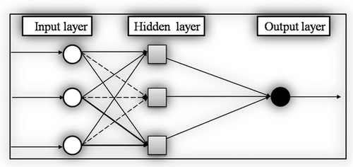
Kim and Valdés (2003) indicated that MLP is capable of simulating 90% of the processes associated with climate. The Levenberg-Marquardt algorithm is the fastest method implemented in MATLAB that has high performance for neural network training (Huang et al. 2006). Therefore, in this study, the Levenberg-Marquardt (LM) method was used as the training algorithm in the MLP to obtain the weight of the network, and the Logsig and Purelin transfer functions were applied to the hidden layer and output layer. The number of hidden neurons was determined by trial and error.

The input data for ANFIS and MLP were divided into training, validation and testing sets in the proportions 70, 15 and 15%, respectively. Then the SPI time series was predicted using climate indices up to four seasons ahead. Following the results of Hsu et al. (1995), the best range for data normalization is 0.05–0.95, as follows:

(5)

where, X_norm and X are the normalized and the original inputs, and X_min and X_max are the minimum and maximum of input ranges, respectively.

In this paper, the models were evaluated using the root mean square error (RMSE), mean absolute error (MAE) and correlation coefficient (R); these error statistics were calculated using the following formulae:

(6)

(7)

(8)

where N is the number of data points, O_i and P_i are the observed and predicted values, respectively, and are the means of the observed and predicted values, respectively.

3 Results

3.1 PCA results

The Kaiser-Meyer-Olkin (KMO) statistical measure (see Section 2.2) was found to be 0.69 in the present study, so the input variables are suitable for the PCA method (Shrestha and Kazama 2007). In the PCA method, components that have eigenvalues greater than 1 are selected as the most important components in explaining the variance. The PCA method showed that eight of the 25 principal component axes had eigenvalues greater than 1 and altogether accounted for 81% of the total variance. Eight components were selected based on the best factor loading (% of the variation) after the varimax rotation. Therefore, the AMO, AMM, BEST, NINO3.4, NINO4, NTA, SOI and TNA indices were selected as the most effective climate signals with factor loading of 0.904, 0.826, 0.952, 0.918, 0.855, 0.908, –0.849 and 0.927, respectively.

3.2 Cross-correlation and MLR prediction results

The results of cross-correlation revealed that AMO, AMM, NTA, SOI and TNA indices have a negative relationship with SPI, while BEST, NINO3.4 and NINO4 have a positive relationship with SPI time series. Among these indices, correlation of the AMO, NINO3.4, NINO4, NTA and TNA with SPI time series is significant at the 5% level of confidence (all of the meaningful indices are related with SPI at different lag-times (Table 1) but not simultaneously). The goal of the cross-correlation function (CCF) is to determine the best time lag for independent variables that have the most influence on the dependent variable (Sigaroodi et al. 2014). So, we considered a MLR equation by using these significant climate indices at different lag times. Stepwise MLR was applied on the training set to develop a linear model. According to the analysis of variance, the F ratio (ratio of the mean square regression to the mean square residual) was equal to 8.301, with a P value of 0.005. The P value (0.005) reflects that our observed F ratio is greater than the F critical value (P value for the regression effect is less than 0.01). Therefore, the regression effect is greater than zero and at least one of the predictors accurately forecasts precipitation. The results for the MLR analysis are shown in Table 2. The indices NINO3.4, NINO4, NTA, TNA and regression constant were excluded from the MLR equation, because a significant number of these indices are less than 0.05, whereas the AMO signal is greater than 0.05. So the MLR equation can be presented with only the AMO signal. Beta is the standard regression coefficient, which helps to clarify the effect of independent variables in the deviations of dependent variables (Beta for the AMO signal is equal to –0.243). Therefore, the MLR equation could be presented in the following form:

(9)

If the VIF value for the AMO signal is equal to one, that indicates no intercorrelation exists. The histogram and normal P-P plot were used to ensure the normality of regression residuals. After establishing the MLR equation, its performance was checked with the remaining 20% of the data. Values of RMSE, MAE and R obtained for training data equal 0.931, 0.723 and 0.242, respectively while for testing data they are 0.993, 0.792 and 0.180, respectively.

Table 1. Results of cross-correlation between seasonal SPI time series and climate signals.

Factor	AMO	AMM	BEST	NINO3.4	NINO4	NTA	SOI	TNA
Cross-correlation coefficient, CC	−0.158	−0.146	0.141	0.166	0.202	−0.184	−0.141	−0.164
Lag time	4	4	0	1	0	4	0	4
Variance	0.077	0.077	0.076	0.076	0.076	0.078	0.078	0.078
Number of data	172	172	172	172	172	172	172	172
Degree of freedom	170	170	170	170	170	170	170	170
T	−2.09	−1.92	1.87	2.19	2.69	−2.44	−1.86	−2.17
P value	0.05	0.1	0.1	0.05	0.01	>0.02	0.1	>0.05

Table 2. Coefficient of stepwise regression and significance testing.

Predictors	β	Beta	T	Significance	VIF
Constant	−0.062		−0.646	0.519
AMO	−1.287	−0.243	−2.881	0.005	1.000
NINO3.4		0.095	1.111	0.269	1.020
NINO4		0.104	1.218	0.225	1.024
NTA		−0.135	−0.977	0.331	2.687
TNA		−0.072	−0.505	0.615	2.854

3.3 Results of MLP and ANFIS models

Since the effect of climate signals on precipitation in different areas is not simultaneous and usually depends on the remoteness of the origin of the climate signals, we tested various input combinations from t to (t − 4) in the MLP and ANFIS models, and prediction intervals were performed simultaneously and up to four seasons ahead. Table 3 shows the structure of input, corresponding output and prediction of MLP and ANFIS models up to four seasons ahead.

Table 3. Structure of input, output and prediction of MLP and ANFIS models.

Inputs	Outputs	Predictions
AMOt, AMMt, NTAt, TNAt, BESTt, NINO3.4t, NINO4t, SOIt	SPIt	SPIt
AMOt-1, AMMt-1, NTAt-1, TNAt-1, BESTt-1, NINO3.4t-1, NINO4t-1, SOIt-1	SPIt	SPIt, SPIt+1
AMOt-2, AMMt-2, NTAt-2, TNAt-2, BESTt-2, NINO3.4t-2, NINO4t-2,, SOIt-2	SPIt	SPIt, SPIt+1, SPIt+2
AMOt-3, AMMt-3, NTAt-3, TNAt-3, BESTt-3, NINO3.4t-3, NINO4t-3, SOIt-3	SPIt	SPIt, SPIt+1, SPIt+2, SPIt+3
AMOt-4, AMMt-4, NTAt-4, TNAt-4, BESTt-4, NINO3.4t-4, NINO4t-4, SOIt-4	SPIt	SPIt, SPIt+1, SPIt+2, SPIt+3, SPIt+4

The performance of MLP and ANFIS models using three global statistics (RMSE, MAE and correlation coefficient, R) is shown in Table 4, together with optimal number of membership functions and hidden nodes. The ANFIS model has the best accuracy (RMSE = 1.02, MAE = 0.78) for the 4-steps-ahead forecasting, while the MLP shows the best performance (RMSE = 0.86, MAE = 0.74) for the 1-step-ahead SPI forecasting. Table 4 clearly indicates that in the training stage the ANFIS models have much better accuracy than the MLP models. In the validation and testing stages, however, the MLP models perform better than the ANFIS models. The SPI RMSE prediction accuracies in the test stage were increased by MLP to 37, 22, 26, 18 and 3% for the t, t + 1, t + 2, t + 3 and t + 4 step ahead forecasts, respectively.

Table 4. Performance of ANFIS and MLP models for prediction of SPI time series.

Model	Number of membership function or intermediate neuron	Step ahead	Training			Validation			Testing
			RMSE	MAE	R	RMSE	MAE	R	RMSE	MAE	R
ANFIS	4	0 (t)	0.48	0.35	0.83	2.52	1.86	0.05	1.42	1.06	0.35
	3	1 (t + 1)	0.70	0.55	0.58	1.80	1.37	0.07	1.10	0.87	0.37
	2	2 (t + 2)	0.73	0.57	0.53	1.18	0.93	0.43	1.33	1.02	0.23
	3	3 (t + 3)	0.63	0.50	0.69	1.33	1.04	0.08	1.19	0.96	0.06
	2	4 (t + 4)	0.73	0.61	0.54	1.35	1.02	0.11	1.02	0.78	0.30
MLP	20	0 (t)	0.83	0.65	0.32	1.13	0.85	0.29	0.89	0.72	0.52
	20	1 (t + 1)	0.81	0.64	0.36	1.00	0.80	0.53	0.86	0.74	0.52
	18	2 (t + 2)	0.80	0.64	0.38	1.16	0.90	0.34	0.98	0.76	0.28
	8	3 (t + 3)	0.80	0.63	0.40	1.09	0.82	0.49	0.98	0.76	0.28
	10	4 (t + 4)	0.84	0.66	0.26	1.24	0.94	0.16	0.99	0.75	0.37

3.4 Comparison of MLR, MLP and ANFIS models

Comparison of MLR, MLP and ANFIS models by RMSE and R statistics is presented in Figure 4, which clearly shows that the MLP network has lower RMSE and higher coefficient of correlation than the ANFIS and MLR models in all forecasting intervals. The MLR model is only able to provide forecasts for four seasons ahead due to the fact that the MLR relationship (equation (9)) was constructed with the AMO signal that is significant with an SPI time series at the 5% level of confidence in the 4-seasons-ahead forecast (t + 4). Also, the best performance of the ANFIS model is in the (t + 4) forecast (RMSE = 1.02, MAE = 0.78 and R = 0.3). From the results of Table 4 and Fig. 4(a) and (b), it can also be seen that the best performance of MLP occurred in the 1-season-ahead forecast (t + 1) (RMSE = 0.86, MAE = 0.74 and R = 0.52).

Figure 4. Comparison of (a) RMSE and (b) R for the MLR, MLP and ANFIS models.

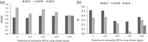
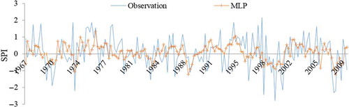
Figures 5–7 show the best performance of the MLR, ANFIS and MLP forecasts, respectively, compared with the observations. Figure 5 clearly shows low performance of MLR to predict the SPI fluctuations, whereas ANFIS and MLP performances are satisfactory (Figs 5 and 6). So, it seems that forecasting of SPI with climate signals using the nonlinear methods is more efficient.

Figure 5. Comparison of the observed and predicted SPI using MLR in the 4-season-ahead forecast (the best performance of the MLR).

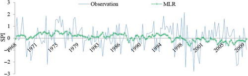
Figure 6. Comparison of the observed and predicted SPI using ANFIS in the 4-season-ahead forecast (the best performance of the ANFIS).

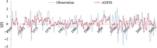
Figure 7. Comparison of the observed and predicted SPI using MLP in the 1-season-ahead forecast (the best performance of the MLP).

4 Discussion

Hydrological modelling in different regions is a critical issue that attracts much attention all over the world. In this study, three types of models were constructed and tested for predicting seasonal SPI time series (MLR, MLP and ANFIS models). Combinations of input data were explored with the PCA method. In order to assess influences of the climate signals on the SPI time series, cross-correlation analysis was used (Karabork et al. 2005) (Table 1). Based on Sigaroodi et al. (2014) only significant indices with SPI time series were used to construct a regression model. The regression model was constructed with AMO signals that gave significant values of the t statistic and P value. The Beta statistic clarifies the importance of AMO signals in the description of SPI time series (for AMO signals, Beta_AMO = −0.243 is the highest). In previous studies, such as Courville and Thompson (2001), Zientek et al. (2008), it was noted that Beta weights in MLR are highly dependent on the variable importance. The VIF value for the AMO signal is equal to 1. This means that no intercorrelation exists between the independent variables. Thus, the model could be considered as an optimal regression equation. This equation was constructed with signals from four previous seasons (because cross-correlation showed that the AMO index had a significant relationship with SPI time series for four steps ahead) to predict 4-season ahead SPI.

Performance evaluation indicated that the MLP network and ANFIS model gave better results than the MLR (Figs 4–7). This is in agreement with the results of Trafalis et al. (2002), Valverde Ramírez et al. (2005), Chattopadhyay (2007) and Dahamsheh and Aksoy (2009), who demonstrated that the ANN was superior to the linear regression model in rainfall forecasting.

This study indicated that the regression model cannot predict the standard deviation or fluctuations of observational data (Fig. 5). So, MLR is not capable of forecasting wet years and droughts. Azadi and Sepaskhah (2012) suggested that neural networks did not significantly increase prediction accuracy compared with MLR.

Dastorani et al. (2010) concluded that the potential of ANN in dry land precipitation forecasting is almost same as with the ANFIS model. In the present study, error parameters in Table 4 and Figure 4 indicate that the MLP models were found to be better than the ANFIS models in predicting SPI time series, which is in agreement with the results of Abyaneh et al. (2011). The main reason is the fact that the ANFIS models use a gradient descent algorithm for calculating the membership function parameters, while the MLP networks use the Levenberg-Marquardt method, which is more powerful and faster than the gradient descent algorithm. Also, the ANFIS model can overlearn during training, resulting in reduced performance during testing.

It seems the relationship between precipitation and climate signals is nonlinear. Thus, a linear method is only able to provide prediction for four seasons ahead, which does not mean good performance. In contrast, the cross-correlation analysis resulted in meaningful correlation coefficients between SPI and climate signals in some cases, but values were not high (i.e. from –0.184 to 0.202) (Table 1). Therefore, the nonlinear relationship between precipitation and climate signals can be considered the reason for the superiority of MLP and ANFIS over MLR.

5 Conclusion

This paper compares several modelling techniques for predicting seasonal SPI from climate signal datasets and describes an approach based on PCA and cross-correlation. In this study, all the climatic indices were used for precipitation forecasting, whereas previous literature did not consider all signals as inputs. The combination of optimal input data to construct a reliable model was determined by using the PCA method. The cross-correlation analysis was used to investigate the relationship between SPI and climate indices for the construction of a stepwise MLR equation. The prediction results showed that the MLP network and ANFIS models performed better than the MLR model. The ANFIS model results were found to be more reliable than those of the MLP model in the training period, but the MLP model showed better accuracy in both validation and testing periods. Thus, it can be concluded that the MLP model is the most suitable model for the studied area.

Uncertainty is one of the most important issues in dealing with weather data that can influence a model’s performance. Although the MLP network had better performance than the ANFIS model, the ANFIS model, due to its fuzzy logic ability, is able to reduce and manage the uncertainty. Therefore, it is necessary to consider the ANFIS model in future studies. For this reason, and because determination of the model structure and input is important in achieving reliable outputs, it is recommended to find the optimum combination and length of data using some other nonlinear methods such as genetic algorithm (GA), gamma test and particle swarm optimization (PSO) in order to improve the prediction accuracy. Many researchers use mathematical models to forecast climate processes, but little has been done to compare the models. It is hoped that this research could be a useful source of important information for other modellers.

Acknowledgements

The authors would like to thank the anonymous reviewers, Professor Demetris Koutsoyiannis and Dr Florian Pappenberger for their constructive scientific comments and feedback.

Disclosure statement

No potential conflict of interest was reported by the authors.

References

- Abtew, W., Melesse, M.A., and Dessalegne, T., 2009. El Nino southern oscillation link to the Blue Nile River Basin hydrology. Hydrological Process, 23 (26), 3653–3660.
- Abyaneh, H.Z., et al., 2011. Performance evaluation of ANN and ANFIS models for estimating garlic crop evapotranspiration. Journal of Irrigation and Drainage Engineering, 137 (5), 280–286. doi:10.1061/(ASCE)IR.1943-4774.0000298
- Azadi, S. and Sepaskhah, A.R., 2012. Annual precipitation forecast for west, southwest, and south provinces of Iran using artificial neural networks. Theoretical and Applied Climatology, 109 (1–2), 175–189. doi:10.1007/s00704-011-0575-9
- Berg, N., et al., 2013. El Niño-Southern Oscillation impacts on winter winds over Southern California. Climate Dynamics, 40 (1–2), 109–121. doi:10.1007/s00382-012-1461-6
- Cañón, J., González, J., and Valdés, J., 2007. Precipitation in the Colorado River Basin and its low frequency associations with PDO and ENSO signals. Journal of Hydrology, 333 (2–4), 252–264. doi:10.1016/j.jhydrol.2006.08.015
- Chattopadhyay, S., 2007. Feed forward artificial neural network model to predict the average summer monsoon rainfall in India. Acta Geophysica, 55 (3), 369–382. doi:10.2478/s11600-007-0020-8
- Chiu, S.L., 1994. Fuzzy model identification based on cluster estimation. Journal of Intelligent and Fuzzy Systems, 2 (3), 267–278.
- Courville, T. and Thompson, B. 2001. Use of structure coefficients in published multiple regression articles: β is not enough. Educational and Psychological Measurement, 61 (2), 229–248. doi:10.1177/0013164401612006
- Dahamsheh, A. and Aksoy, H., 2009. Artificial neural network models for forecasting intermittent monthly precipitation in arid regions. Meteorological Applications, 16 (3), 325–337. doi:10.1002/met.127
- Dastorani, M.T., et al., 2010. Application of ANN and ANFIS models on dryland precipitation prediction (Case study: Yazd in Central Iran). Journal of Applied Sciences, 10 (20), 2387–2394. doi:10.3923/jas.2010.2387.2394
- El-Shafie, A., Jaafer, O., and Seyed, A., 2011. Adaptive neuro-fuzzy inference system based model for rainfall forecasting in Klang River, Malaysia. International Journal of the Physical Sciences, 6 (12), 2875–2888.
- Fallah-Ghalhary, G.A., et al., 2010. Spring rainfall prediction based on remote linkage controlling using adaptive neuro-fuzzy inference system (ANFIS). Theoretical and Applied Climatology, 101 (1–2), 217–233. doi:10.1007/s00704-009-0194-x
- Famini, G.R., Penski, C.A., and Wilson, L.Y., 1992. Using theoretical descriptors in quantitative structure activity relationships: some physicochemical properties. Journal of Physical Organic Chemistry, 5 (7), 395–408. doi:10.1002/poc.610050704
- Faria, R., Duncan, J.C., and Brereton, R.G., 2007. Dynamic mechanical analysis and chemometrics for polymer identification. Polymer Testing, 26 (3), 402–412. doi:10.1016/j.polymertesting.2006.12.012
- Farokhnia, A., Morid, S., and Byun, H.-R., 2011. Application of global SST and SLP data for drought forecasting on Tehran plain using data mining and ANFIS techniques. Theoretical and Applied Climatology, 104 (1–2), 71–81. doi:10.1007/s00704-010-0317-4
- Firat, M. and Güngör, M., 2007. River flow estimation using adaptive neuro fuzzy inference system. Mathematics and Computers in Simulation, 75, 87–96. doi:10.1016/j.matcom.2006.09.003
- Gámiz-Fortis, S.R., et al., 2010. Potential predictability of an Iberian river flow based on its relationship with previous winter global SST. Journal of Hydrology, 385 (1–4), 143–149. doi:10.1016/j.jhydrol.2010.02.010
- Grantz, K., et al., 2005. A technique for incorporating large-scale climate information in basin-scale ensemble stream flow forecasts. Water Resources Research, 41 (10), 1–13. doi:10.1029/2004WR003467
- Günaydın, O., 2009. Estimation of soil compaction parameters by using statistical analyses and artificial neural networks. Environmental Geology, 57 (1), 203–215. doi:10.1007/s00254-008-1300-6
- Hsu, K.-L., Gupta, H.V., and Sorooshian, S., 1995. Artificial neural network modeling of the rainfall-runoff process. Water Resources Research, 31 (10), 2517–2530. doi:10.1029/95WR01955
- Huang, G.-B., Zhu, Q.-Y., and Siew, C.-K., 2006. Extreme learning machine: theory and applications. Neurocomputing, 70 (1–3), 489–501. doi:10.1016/j.neucom.2005.12.126
- Jang, J.-S.R., 1993. ANFIS: adaptive-network-based fuzzy inference system. IEEE Transactions on Systems, Man, and Cybernetics, 23 (3), 665–685. doi:10.1109/21.256541
- Jang, J.-S.R. and Sun, C.-T., 1995. Neuro-fuzzy modeling and control. Proceedings of the IEEE, 83 (3), 378–406. doi:10.1109/5.364486
- Jeong, C.H., et al., 2012. Monthly precipitation forecasting with a neuro-fuzzy model. Water Resources Management, 26 (15), 4467–4483. doi:10.1007/s11269-012-0157-3
- Jolliffe, I.T., Jones, B., and Morgan, B.J.T., 1980. Cluster analysis of the elderly at home: a case study. In: E. Diday et al., eds. Data analysis and informatics. Amsterdam: North-Holland, 745–757.
- Kaiser, H.F., 1970. A second generation little jiffy. Psychometrika, 35, 401–415. doi:10.1007/BF02291817
- Kaiser, H.F., 1974. An index of factorial simplicity. Psychometrika, 39, 31–36. doi:10.1007/BF02291575
- Kalra, A. and Ahmad, S., 2009. Using oceanic–atmospheric oscillations for long lead time streamflow forecasting. Water Resources Research, 45 (3), 1–18. doi:10.1029/2008WR006855
- Kalra, A., et al.,2013. Using large-scale climatic patterns for improving long lead time streamflow forecasts for Gunnison and San Juan River Basins. Hydrological Processes, 27 (11), 1543–1559. doi:10.1002/hyp.9236
- Karabork, M.C., Kahya, E., and Karaca, M., 2005. The influences of the Southern and North Atlantic Oscillations on climatic surface variables in Turkey. Hydrological Processes, 19 (6), 1185–1211. doi:10.1002/hyp.5560
- Kim, T. and Valdés, J., 2003. Nonlinear model for drought forecasting based on a conjunction of wavelet transforms and neural networks. Journal of Hydrologic Engineering, 8 (6), 319–328. doi:10.1061/(ASCE)1084-0699(2003)8:6(319)
- Kim, T.-W., Yoo, C., and Ahn, J.-H., 2008. Influence of climate variation on seasonal precipitation in the Colorado River Basin. Stochastic Environmental Research and Risk Assessment, 22 (3), 411–420. doi:10.1007/s00477-007-0126-1
- Kisi, O. and Shiri, J., 2011. Precipitation forecasting using wavelet-genetic programming and wavelet-neuro-fuzzy conjunction models. Water Resources Management, 25 (13), 3135–3152. doi:10.1007/s11269-011-9849-3
- Kumar, D.N., Reddy, M.J., and Maity, R., 2007. Regional rainfall forecasting using large scale climate teleconnections and artificial intelligence techniques. Journal of Intelligent Systems, 16 (4), 307–322.
- Kurtulus, B. and Razack, M., 2010. Modeling daily discharge responses of a large karstic aquifer using soft computing methods: artificial neural network and neuro-fuzzy. Journal of Hydrology, 381 (1–2), 101–111. doi:10.1016/j.jhydrol.2009.11.029
- Quraishi, M.Z. and Mouazen, A.M., 2013. Development of a methodology for in situ assessment of topsoil dry bulk density. Soil and Tillage Research, 126, 229–237. doi:10.1016/j.still.2012.08.009
- Ringnér, M., 2008. What is principal component analysis? Nature Biotechnology, 26 (3), 303–304. doi:10.1038/nbt0308-303
- Rumelhart, D.E., Hinton, G.E., and Williams, R.J., 1986. Learning representations by back-propagating errors. Nature, 323, 533–536. doi:10.1038/323533a0
- Sanikhani, H. and Kisi, O., 2012. River flow estimation and forecasting by using two different adaptive neuro-fuzzy approaches. Water Resources Management, 26 (6), 1715–1729. doi:10.1007/s11269-012-9982-7
- Seleshi, Y. and Zanke, U., 2004. Recent changes in rainfall and rainy days in Ethiopia. International Journal of Climatology, 24 (8), 973–983. doi:10.1002/joc.1052
- Shrestha, S. and Kazama, F., 2007. Assessment of surface water quality using multivariate statistical techniques: a case study of the Fuji river basin, Japan. Environmental Modelling and Software, 22 (4), 464–475. doi:10.1016/j.envsoft.2006.02.001
- Sigaroodi, S.K., et al., 2014. Long-term precipitation forecast for drought relief using atmospheric circulation factors: a study on the Maharlu Basin in Iran. Hydrology and Earth System Sciences, 18 (5), 1995–2006. doi:10.5194/hess-18-1995-2014.
- Takagi, T. and Sugeno, M., 1985. Fuzzy identification of systems and its applications to modeling and control. IEEE Transactions on Systems, Man, and Cybernetics, SMC-15 (1), 116–132. doi:10.1109/TSMC.1985.6313399
- Tomassetti, B., Verdecchia, M., and Giorgi, F., 2009. NN5: A neural network based approach for the downscaling of precipitation fields – model description and preliminary results. Journal of Hydrology, 367 (1–2), 14–26. doi:10.1016/j.jhydrol.2008.12.017
- Trafalis, T.B., et al., 2002. Data mining techniques for improved WSR-88D rainfall estimation. Computers & Industrial Engineering, 43 (4), 775–786. doi:10.1016/S0360-8352(02)00139-0
- Turkes, M. and Elart, E., 2003. Precipitation changes and variability in Turkey linked to the North Atlantic oscillation during the period 1930-2000. International Journal of Climatology, 23 (14), 1771–1796. doi:10.1002/joc.962
- Valverde Ramírez, M.C., De Campos Velho Maria, H.F., and Ferreira, N.J., 2005. Artificial neural network technique for rainfall forecasting applied to the São Paulo region. Journal of Hydrology, 301 (1–4), 146–162. doi:10.1016/j.jhydrol.2004.06.028
- Wallace, J.M., 2000. North Atlantic oscillation/annular mode: two paradigms -one phenomenon. Quarterly Journal of the Royal Meteorological Society, 126 (564), 791–805. doi:10.1256/smsqj.56401
- Zientek, L.R., Capraro, M.M., and Capraro, R.M., 2008. Reporting practices in quantitative teacher education research: one look at the evidence cited in the AERA panel report. Educational Researcher, 37 (4), 208–216. doi:10.3102/0013189X08319762