Testing the applicability of a kinematic wave-based distributed hydrological model in two climatically contrasting catchments

Abstract

Steep mountainous areas account for 70% of all river catchments in Japan. To predict river discharge for the mountainous catchments, many studies have applied distributed hydrological models based on a kinematic wave approximation with surface and subsurface flow components (DHM-KWSS). These models reproduce observed river discharge of catchments in Japan well; however, the applicability of a DHM-KWSS to catchments with different geographical and climatic conditions has not been sufficiently examined. This research applied a DHM-KWSS to two river basins that have different climatic conditions from basins in Japan to examine the transferability of the DHM-KWSS model structure. Our results show that the DHM-KWSS model structure explained flow regimes for a wet river basin as well as a large flood event in an arid basin; however, it was unable to explain long-term flow regimes for the arid basin case study.

Résumé

Les zones de montagne pentues comptent pour 70% des bassins au Japon. Afin de prévoir les débits pour les bassins montagneux, de nombreuses études ont appliqué des modèles hydrologiques distribués basés sur une approximation de l’onde cinématique avec des composantes de flux de surface et de subsurface (DHM-KWSS). Ces modèles reproduisent les débits observés des bassins japonais de manière précise; toutefois, l’applicabilité d’un DHM-KWSS à des bassins ayant des conditions géographiques et climatiques différentes n’a pas été suffisamment étudiée. La présente recherche concerne l’application d’un DHM-KWSS à deux bassins qui subissent des conditions climatiques différentes de celles du Japon afin d’examiner la transférabilité de la structure d’un modèle DHM-KWSS. Nos résultats montrent que la structure du modèle DHM-KWSS explique les régimes pour un bassin humide ainsi que les évènements de crues important pour un bassin aride; en revanche, il n’est pas capable d’expliquer les régimes à long terme pour le bassin aride étudié.

Key words:

• distributed rainfall–runoff models
• the Garonne River
• the Flinders River
• kinematic wave model

Mots clefs:

• modèles pluie–débits distribués 
• la rivière Garonne
• la rivière Flinders
• modèle d’onde cinématique

1 INTRODUCTION

To develop a suitable hydrological model to forecast river flows, the dominant hydrological processes in a catchment must be identified. To contribute to such fundamental hydrological research, a Workshop Testing simulation and forecasting models in non-stationary conditions was held during the 2013 IAHS conference in Göteborg, Sweden (Thirel et al. 2015). Workshop participants selected target basins and simulated long-term river discharge using several rainfall–runoff and land-surface models with the meteorological data provided, and we discussed the transferability of a Distributed Hydrologic Model based on a Kinematic Wave flow approximation (DHM-KWSS) that considers both surface and subsurface flow components).

Many river basins in Japan have steep slopes, being located in mountainous terrain, which causes rapid propagation of flood flows. These slopes are mainly covered by forests, which in temperate climatic conditions keep soil moisture in the surface layer. Rainfall–runoff processes in these climatic conditions have been represented by some DHM-KWSS, such as HydroBEAM (Kojiri et al. 2008) and OHDIS-KWMSS (Takasao and Shiiba 1988, Sayama et al. 2006, Sayama and McDonnell 2009, Kim et al. 2011). Hunukumbura et al. (2012) used a DHM-KWSS to describe short-term flood events in several river basins located in multiple countries, encompassing a range of geographic and climatic conditions different from those in Japan. This study showed that the model was applicable to basins with steep slopes and a temperate climate condition similar to those in Japan; however, it has difficulty describing hydrological behaviour in arid climates as well as those with mild topography.

This study applied a DHM-KWSS for long-term simulations including periods of flood and drought to further understand the transferability of the model structure. Applying a DHM-KWSS over a long time period is intended to test the model structure under a variety of hydrological conditions. In this study, 1K-DHM (Tachikawa and Tanaka 2013), which is a distributed hydrological models with the DHM-KWSS structure, was applied to two river basins. One was the area upstream of Portet-sur-Garonne in the Garonne River basin (9980 km²) in southern France; the other was the area upstream of Glendower in the Flinders River basin (1960 km²) in northern Australia. The Garonne River basin is characterized by relatively stable rainfall throughout the year, which is similar to climatic conditions in Japanese river basins. The Flinders River basin is located in an arid area which is climatically quite different. To examine the applicability of the DHM-KWSS model structure for basins with different climates and topography, model parameters were calibrated, and then the calibrated model was examined with observed discharge. Model validation showed that the DHM-KWSS model structure successfully describes flow regimes in the catchment upstream of Portet-sur-Garonne in the Garonne River basin. For the catchment above Glendower in the arid Flinders River basin, extreme flood events were well reproduced, but it was difficult to represent long-term flow regimes.

2 MODEL FRAMEWORK

The 1K-DHM is a distributed hydrological model based on a kinematic wave flow approximation that considers subsurface flow. This model uses a kinematic wave model that describes surface and subsurface flow using a storage–discharge equation. As shown in Fig. 1, kinematic flow is applied to each cell within 1K-DHM, where flow is calculated using rainfall input to the cell and discharge from upper cells as the boundary condition. Flow direction is determined using topographical data provided by HydroSHEDS (http://hydrosheds.cr.usgs.gov).

Fig. 1 Schematic drawing of flow simulation in 1K-DHM.

As shown in Fig. 2, each cell is contributed to by its upslope cells and the number of upslope cells S is determined by the flow direction. If S is larger than the threshold S₀, which is set to 250 in this study, the cell is considered a river-channel cell; otherwise, it is classified as a slope-runoff cell. A threshold value of 250 was found to reproduce the observed river discharge in some Japanese river basins. The following kinematic wave model represents flow for river-channel cells:

(1)

(2)

Fig. 2 Definition of slope, river channel and rill cells in 1K-DHM (dark grey: river cells, light grey: rill cells, white: slope cells).

where A is the cross-sectional area; Q is discharge; r is rainfall intensity; e is evapotranspiration; and α_c and m are parameters. These parameters are determined as α_c = √i /n_cB^−3/2 and m = 3/5, assuming a rectangular cross-section of each cell. The parameters i, n_c and B represent the slope gradient, Manning’s roughness coefficient, and the width of river channel, respectively. The value of B is determined by B = bS^c, where b = 1.06 and c = 0.69. These values were determined by considering the behavior of many observation stations across Japan.

Flow from slope-runoff for each cell is modelled by the following two equations, which consider both saturated and unsaturated subsurface flow components (Hunukumbura et al. 2012):

(3)

(4)

where h is water stage; q is discharge per unit slope width; d_c is a water stage equivalent to the maximum water content in capillary pores; k_c is hydraulic conductivity when the capillary pores are saturated; β is an exponent parameter that describes the relationship between hydraulic conductivity and saturation; k_a is saturated hydraulic conductivity and k_a = βk_c according to the continuity of the q–h relationship (equation (4)); d_a is the water stage equivalent to the maximum water content in the effective porosity; and n_s is Manning’s roughness coefficient for overland flow in slope runoff cells. equation (4) represents the q–h relationship for the surface and subsurface soil layer, as shown in Fig. 3. When the cross-section A or the slope water depth h becomes negative due to the negative input (the r – e portion of equations (1) and (3)), both values are set to zero.

Fig. 3 Discharge-storage function of slope cells.

Some portions of mountainous slopes are composed of gullies, where compacted bare ground causes quick surface flow. The model represents these areas as rill cells with no subsurface soil layers. Arid catchments are assumed to contain these impervious areas, which strongly affect flow regimes. To introduce the rill cells into the model, a slope-runoff cell with the number of upslope cells S that is larger than the threshold S₁ and smaller than S₀ is set as a rill cell. Water flow in these rill cells is calculated using equations (3) and (4), in which soil layer parameters (specifically d_a and d_c) are set to zero. In other words, the basic equation is equivalent to equations (1) and (2), with the condition that Manning’s coefficient is equal to n_s. The property of the rill cells is important in simulating the Flinders River, as described in the following section.

3 APPLYING 1K-DHM TO TWO TEST BASINS

3.1 Application framework

The 1K-DHMl model, as described above, was applied to the Garonne River in France and the Flinders River in Australia. Following the protocol established for the Workshop described by Thirel et al. (2015), the entire period was divided into five sub-periods for each basin, as shown in Table 1. Each period was named Pi (where i = 1, 2, 3, 4, 5), and the complete period was named P6. First, the parameters of 1K-DHM were calibrated for each time period P1–P6. For the calibration, the SCE-UA algorithm (Duan et al. 1994) was used to optimize parameters, and the Nash-Sutcliffe coefficient was used to evaluate the model efficiency. This resulted in six calibrated parameter sets for P1–P6, termed θ1–θ6 herein. Secondly, the six parameter sets were applied to 1K-DHM to simulate river discharge outside of the time periods used for calibration.

Table 1 Duration of the six periods used for calibration and validation for the Garonne and Flinders rivers.

Period	River Garonne	River Flinders
P1	1961–1969	1973–1979
P2	1970–1978	1980–1986
P3	1979–1987	1987–1993
P4	1988–1996	1994–2000
P5	1997–2005	2001–2007
P5	1961–2005	1973–2007

3.2 River basin conditions

The catchment area upstream of Portet-sur-Garonne in the Garonne River basin (9980 km²) and the area upstream of Glendower in the Flinders River basin (1960 km²) were selected as the study basins. The former catchment has similar climatic conditions to Japanese river basins, while the latter has very different climatic conditions to the Garonne River basin and most basins in Japan. The Garonne River catchment is characterized by a mean annual precipitation of about 1200 mm, where precipitation occurs consistently throughout the year. However, the Flinders River catchment, located in northern Australia, has a semi-arid tropical climate, with drastic inter-annual variability in precipitation. The mean annual precipitation in this catchment is about 600 mm, and flood events occur mainly in the wet season from November to April. Rainfall during this period accounts for 80% of annual precipitation. During the dry season, precipitation is not enough to maintain this ephemeral river, which has no flow in dry months.

Figures 4 and 5 show the watershed boundaries of the Garonne and Flinders river basins, which were obtained from topographic data in HydroSHEDS. The light-shading delineates the entire river basin in each case, while the dark-grey colour shows the study catchments upstream of Portet-sur-Garonne and Glendower. The right side of Figs 4 and 5 indicates the spatial distribution of slope gradient as calculated from topographic data. In both catchments, almost all cells have a gradient larger than 0.01; this means that both satisfy the topological conditions of 1K-DHM based on a kinematic wave flow approximation.

Fig. 4 Left: watershed boundary of the Garonne River basin (black line: river channel grids, light grey: the whole area of the Garonne River basin, dark grey: catchment upstream of Portet-sur-Garonne). Right: spatial distribution of slope gradient of catchment upstream of Portet-sur-Garonne.

Fig. 5 Left: watershed boundary of the Flinders River basin (black line: river channel grids, grey line: rill grids, light grey area: the whole Flinders River basin, dark grey area: catchment upstream of Glendower). Right: spatial distribution of slope gradient of catchment upstream of Glendower.

3.3 Observed data

Daily precipitation, potential evapotranspiration, and river discharge data were obtained for both basins. For the Garonne River basin, precipitation data were obtained from SAFRAN analysis conducted by Météo France (Quintana-Seguí et al. 2008, Vidal et al. 2010). Potential evapotranspiration was calculated using the Penman-Monteith formula (Penman 1948). Discharge data were obtained from Banque HYDRO, the French hydrological database (http://www.hydro.eaufrance.fr). For the Flinders River basin, precipitation and potential evapotranspiration data estimated by Morton’s method (Morton 1983), were obtained from the SILO climate data archive (http://www.longpaddock.qld.gov.au/silo, Jeffrey et al. 2001). River discharge was provided by the State of Queensland (http://watermonitoring.derm.qld.gov.au/host.htm).

To illustrate the flow regime characteristics of the Garonne and Flinders rivers, observed daily discharge hydrographs at Portet-sur-Garonne in 1982, and at Glendower in 1981, are shown in Fig. 6. The Garonne River has continuous flow throughout the year, and relatively high discharge appears after the winter season. Conversely, the Flinders River has very low flow for most of the year except during the wet season from January to March. The ratio Q_s/P between the total annual runoff Q_s and precipitation P for both catchments is shown in Fig. 7. For the Garonne River the ratio is about 0.5, which means that half of the precipitation contributes to runoff, while for the Flinders, the ratio is about 0.1 throughout the period, indicating that the majority of rainfall infiltrates into the soil layers, or evaporates into the atmosphere.

Fig. 6 Hydrographs of observed discharge of the two basins (grey: Portet-sur-Garonne in the Garonne River basin, black: Glendower in the Flinders River basin).

Fig. 7 The observed ratio of annual runoff to precipitation for the two basins (grey: Portet-sur-Garonne in the Garonne River basin, black: Glendower in the Flinders River basin).

3.4 Estimation of actual evapotranspiration

For long-term runoff simulations, actual evapotranspiration (AET) is required; however, the available data is potential evapotranspiration (PET). Therefore, AET was estimated from PET, as described below. Assuming that the error in the water balance calculated from AET is equal to zero, the error ratio in the annual water balance L_p to precipitation using PET was calculated for both basins to examine how much larger PET is than AET:

(5)

where E_p is total annual potential evapotranspiration. If L_p has a negative value, it shows that PET is larger than AET. The values of L_p for each year at Portet-sur-Garonne (Garonne River) and Glendower (Flinders River) are shown in Fig. 8, which indicates that L_p for the Garonne is approximately −0.4, whereas for the Flinders it ranges from −0.7 to −5.0. It is clear that PET is much larger than AET for the Flinders River basin.

Fig. 8 The observed ratio of annual water balance to precipitation for the two basins (grey: Portet-sur-Garonne in the Garonne River basin, black: Glendower in the Flinders River basin).

To obtain AET, annual actual evapotranspiration E_a was estimated as:

(6)

Assuming E_a = αE_p, α  ≤ 1.0 and substituting this into equation (6), one obtains:

(7)

where the values of α are calculated by:

(8)

Daily actual evapotranspiration is assumed to be:

(9)

where e_a(t) and e_p(t) are daily actual and potential evapotranspiration, respectively; and t represents day.

3.5 Initial conditions

The initial condition of the 1K-DHM is determined by assuming a steady state. At the steady state, river discharge Q at r in each cell is given by:

(10)

where r is intensity of runoff generation at the steady state, and A is the area upstream of the cell. Given the observed initial river discharge at a gauging station Q, r can be calculated by equation (10). The initial river discharge at each cell Q_i with an upstream area of A_i is calculated as Q_i = rA_i.

3.6 Performance index

The Nash-Sutcliffe coefficient in N_s was used as an evaluation criterion for calibration:

(11)

where Q_sim,i is simulated daily discharge, and Q_obs,i is observed daily discharge for the ith day. The validation results were evaluated by calculating N_s and the bias of the total amount of runoff calculated as:

(12)

As most of the daily discharge at Glendower is less than 1 m³/s, the Nash-Sutcliffe coefficient calculated on inverse transformed flows N_l was used (Pushpalatha et al. 2012):

(13)

Both the denominator and numerator of equation (13) involve the inverse of discharge, which indicates that the better the model reproduces low flow, the higher N_l becomes. The parameter γ is added to avoid division by zero.

3.7 Calibration and validation processes

In the calibration stage, the initial conditions were set to each of the six time periods (P1–P6) to reproduce river discharge measured at Portet-sur-Garonne and Glendower. The SCE-UA algorithm then searches these parameter sets with the highest Nash-Sutcliffe coefficient. The parameter sets for both rivers include n_s, k_a, d_a, d_c and β in equation (4), while the Flinders River set also included S₁. For model validation, river discharge hydrographs for the periods P1–P6 were simulated using parameter sets θi (i = 1, 2, …, 6).

4 RESULTS AND DISCUSSION

4.1 The Garonne River basin

Figures 9 and 10 show the Nash-Sutcliffe coefficient and the bias over calibration and validation stages for periods P1–P6, as calculated using parameter sets θ1 to θ6. The results for Pi using parameter sets θi (i = 1, 2, …, 6) are for the calibration, while the other results are for validation. Nash-Sutcliffe coefficient scores calculated for all parameters ranged from 0.4 to 0.7, with an overall bias of almost 1.0, as shown in Table 2.

Table 2 Calibrated parameter values for the River Garonne, the River Flinders, and the Maruyama River catchments in Japan (Hunukumbura et al. 2012).

	Ns (m^3/s)	ka (m/s)	da (m)	dc (m)	β (-)	S1 (-)
River Garonne
θ1	0.222	6.20 × 10^–3	1.05	0.739	6.10	–
θ2	0.161	7.50 × 10^–3	0.781	0.742	2.80	–
θ3	0.170	4.70 × 10^–3	1.62	0.625	9.83	–
θ4	0.240	1.82 × 10^–2	1.00	0.994	5.13	–
θ5	0.117	3.00 × 10^–2	0.797	0.656	9.98	–
θ6	0.175	1.00 × 10^–2	0.811	0.662	3.67	–
River Flinders
θ1	0.0100	4.90 × 10^–3	1.99	0.999	4.15	12
θ2	0.100	2.05 × 10^–2	0.830	0.821	3.98	14
θ3	0.0100	9.20 × 10^–3	1.11	0.975	10.1	22
θ4	0.0126	1.04 × 10^–2	0.881	0.786	6.17	141
θ5	0.0101	1.35 × 10^–2	0.658	0.635	13.0	215
θ6	0.0101	2.69 × 10^–3	2.47	0.878	5.00	47
Maruyama River basin
	0.480	7.00 × 10^–2	0.306	0.0550	16.0	–

Fig. 9 Nash-Sutcliffe coefficient of river discharge using the six parameter sets for each period at Portet-sur-Garonne.

Fig. 10 Bias of observed and simulated discharge by the six parameter sets for each period at Portet-sur-Garonne.

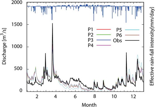
To further understand the Garonne River basin results, for 1982, observed and simulated (using the parameter sets θ1–θ6) discharge hydrographs are shown in Fig. 11. The simulated discharge at Portet-sur-Garonne replicated the behaviour of the overall flow characteristics. Simulated hydrographs for other years followed a similar tendency. The Garonne River basin experiences rainfall for every month, and so the upper soil layer would have enough wetness to cause gravity flow. This characteristic matches the DHM-KWSS structure. To analyse the characteristics of flow from the parameter sets, 1K-DHM parameter values obtained at the Maruyama River basin in Japan (Hunukumbura et al. 2012) are also shown in Table 2. The d_c values identified for the Garonne River basin are larger than for the Maruyama River basin. The 1K-DHM model does not incorporate snow accumulation processes, thus snowmelt is reflected by the large d_c value. If snow accumulation and snowmelt processes are incorporated into 1K-DHM, the d_c value would to be similar to that of the Maruyama River basin. The Nash-Sutcliffe coefficients for the validation periods are about 0.6, and the bias is about 1.05. In addition, the parameter sets in Table 2 do not vary across time periods, which shows that the parameter set is stable for the Garonne River. This supports the notion that the DHM-KWSS model structure is applicable for the Garonne River basin.

Fig. 11 Hydrograph of observed (thick line) and simulated discharge in 1982 at Portet-sur-Garonne (effective rainfall means rainfall minus evapotranspiration).

4.2 The Flinders River basin

The Nash-Sutcliffe coefficients and the bias for both calibration and validation of the Flinders River basin are shown in Figs 12 and 13, respectively. The Nash-Sutcliffe coefficient ranges from 0.4 to 0.6, except for the results from θ5. However, the bias ranges from 1.0 to 3.0, which means that the simulated discharge tends to be overestimated. The calibrated parameters are shown in Table 2.

Fig. 12 Nash-Sutcliffe coefficient of river discharge using the six parameter sets for each period at Glendower.

Fig. 13 Bias of observed and simulated discharge using the six parameter sets for each period at Glendower.

To illustrate these results, the observed and simulated discharge hydrographs from October to December in 1981 at Glendower are shown in Fig. 14. We can see that the simulated peak discharge is overestimated when compared to that observed for almost all events. Simulated results for other years showed a similar tendency. This is due to the uniform ratio parameter α used to estimate actual daily evapotranspiration. The AET was underestimated in the wet season and overestimated in the dry season. To keep river discharge for the dry season, the values of d_a and d_c were identified as being larger for the Flinders River basin than for the Maruyama River basin. The underestimated AET in the wet season then caused overestimation of discharge during the rainy season. The thick soil layers also resulted in delay of the hydrograph peak as observed in Fig. 14. Thus n_s was calibrated to a small value to reduce the delay of peak discharges. The N_l values calculated over all the parameter sets are shown in Fig. 15. These N_l values are negative through the calibration and validation periods, indicating that the low flow reproducibility is poor.

Fig. 14 Hydrograph of observed (thick line) and simulated discharge from October to December in 1981 at Glendower (effective rainfall is rainfall minus evapotranspiration).

Fig. 15 Nash-Sutcliffe coefficient of river discharge for low flow using the six parameter sets for each period at Glendower.

The model efficiency for a large flood event was examined. The observed and simulated hydrographs for the significant flood event caused by the hurricane in 2002 are shown in Fig. 16. The discharge simulated by parameter set θ5 represented well the observed discharge. During period P5, a hurricane hit the Flinders River basin; therefore, compared to the other parameter sets, θ5 has smaller values of d_a and d_c, which means surface flows occur more readily. Indeed, since the basin was dry at the beginning of this hurricane event, the hydraulic conductivity at the soil surface would have been quite small. Thus, the DHM-KWSS model structure was able to represent the extremely large flood.

Fig. 16 Hydrograph of observed (thick line) and simulated discharge of the largest flood event at Glendower in the observation period, caused by a major hurricane in 2002 (effective rainfall is rainfall minus evapotranspiration).

4.3 Summary

The above results show that care must be taken in applying the DHM-KWSS model structure to different catchments. Nash-Sutcliffe coefficients arising from the best-performing parameter set for the Garonne River basin are larger than for the Flinders River basin. The bias calculated for the Garonne River basin shows that the simulated total runoff is close to that observed, while for the Flinders River basin, the simulated total runoff is overestimated. The findings are as follows; the DHM-KWSS model structure expresses flow regimes in the Garonne River basin with temperate climate conditions and large flood events in the Flinders river basin, but flow regimes of arid areas over long time period are not well explained.

5 CONCLUSIONS

River basins in Japan have steep mountainous topography with temperate climatic conditions. These properties have been successfully modelled by the DHM-KWSS model structure. This research examined the applicability of the model 1K-DHM, with a DHM-KWSS model structure, to the Garonne and Flinders river basins. These basins have similar topography to Japanese basins, but encompass a range of climatic conditions. The calibration and validation results showed that the rainfall–runoff process in the Garonne River basin could be explained with the DHM-KWSS model structure; however, it did not describe the arid Flinders River basin well. The findings are summarized as follows:

1. 1K-DHM captures runoff characteristics in the Garonne River basin. This basin experiences rainfall every month and runoff from the basin responds rapidly to rainfall. This behaviour is well described by the DHM-KWSS model structure. Surface and saturated subsurface parameters are similar to those found in Japanese basins. These parameters do not vary in different identification periods, which indicates that the rainfall–runoff processes are expressed by the DHM-KWSS model structure.

2. The simulation scores from the Flinders River basin during the low-flow season were low, and the simulation biases were high. The former means that the model structure in 1K-DHM does not account for rainfall–runoff processes for arid basins, and the latter is explained by the error in estimating interannual variation in actual evapotranspiration. Interestingly, the simulated discharge during the large flood in 2002 was reproduced well using 1K-DHM. This is because the vertical infiltration in the dry season is small, and surface flow accounts for the large flood runoff phenomena. The varying of the calibrated parameters sets across the periods is likely due to insufficient modelling of rainfall–runoff processes in arid basins.

The above conclusions show that the DHM-KWSS model structure expresses flow regimes in a temperate river basin similar to Japanese river basins, as well as flood events in an arid basin. However, this model structure cannot describe flow behaviour for the arid area.

Rainfall–runoff predictions are subject to uncertainties regarding the accuracy of hydrological data, parameter identification and model structure. The Flinders River basin is steep enough to be approximated by a kinematic wave flow approximation, although runoff generation in the arid basin has different hydrological processes from those expressed in DHMs-KWSS. To explain flow regimes over a wider range of basins with different climatic conditions, improving the estimation of snow accumulation and snowmelt, and of actual evapotranspiration inter-annual variability is essential. In addition, future research must focus on optimizing model structures that capture subsurface or underground flow dynamics.

Disclosure statement

No potential conflict of interest was reported by the author(s).

REFERENCES

- Duan, Q., Sorooshian, S., and Gupta, V.K., 1994. Optimal use of the SCE-UA global optimization method for calibrating watershed models. Journal of Hydrology, 158, 265–284. doi:10.1016/0022-1694(94)90057-4
- Hunukumbura, P.B., Tachikawa, Y., and Shiiba, M., 2012. Distributed hydrological model transferability across basins with different physio-climatic characteristics. Hydrological Processes, 26 (6), 793–808. doi:10.1002/hyp.8294
- Jeffrey, S.J., et al., 2001. Using spatial interpolation to construct a comprehensive archive of Australian climate data. Environmental Modelling & Software, 16 (4), 309–330. doi:10.1016/S1364-8152(01)00008-1
- Kim, S., et al., 2011. Climate change impact on river flow of the Tone river basin, Japan. Journal of Japan Society of Civil Engineers, Ser. B1 (Hydraulic Engineering), 67 (4), 85–90.
- Kojiri, T., Hamaguchi, T., and Ode, M., 2008. Assessment of global warming impacts on water resources and ecology of a river basin in Japan. Journal of Hydro-environment Research, 1, 164–175. doi:10.1016/j.jher.2008.01.002
- Morton, F.I., 1983. Operational estimates of areal evapotranspiration and their significance to the science and practice of hydrology. Journal of Hydrology, 66 (1–4), 1–76. doi:10.1016/0022-1694(83)90177-4
- Penman, H.L., 1948. Natural evaporation from open water, bare soil and grass. Proceedings of the Royal Society A: Mathematical, Physical and Engineering Sciences, 193, 120–145. doi:10.1098/rspa.1948.0037
- Pushpalatha, R., et al., 2012. A review of efficiency criteria suitable for evaluating low-flow simulations. Journal of Hydrology, 420-421, 171–182. doi:10.1016/j.jhydrol.2011.11.055
- Quintana-Seguí, P., et al., 2008. Analysis of near-surface atmospheric variables: validation of the SAFRAN analysis over France. Journal of Applied Meteorology and Climatology, 47 (1), 92–107. doi:10.1175/2007JAMC1636.1
- Sayama, T. and McDonnell, J.J., 2009. A new time-space accounting scheme to predict stream water residence time and hydrograph source components at the watershed scale. Water Resources Research, 45, W07401. doi:10.1029/2008WR007549
- Sayama, T., et al., 2006. Distributed rainfall–runoff analysis in a flow regulated basin having multiple multi-purpose dams. In: M. Sivapalan, et al., eds. Predictions in ungauged basins: promises and progress [online]. International Association of Hydrological Sciences, IAHS Publ. 303, 371–381. Available from: http://iahs.info/uploads/dms/13449.46-371-381-S7-37-sayama-et-al.pdf [Accessed 29 April 2015].
- Tachikawa, Y. and Tanaka, T., 2013. 1K-FRM/DHM. Available from: http://hywr.kuciv.kyoto-u.ac.jp/products/1K-DHM/1K-DHM.html [Accessed 29 July 2014].
- Takasao, T. and Shiiba, M., 1988. Incorporation of the effect of concentration of flow into the kinematic wave equations and its applications to runoff system lumping. Journal of Hydrology, 102, 301–322. doi:10.1016/0022-1694(88)90104-7
- Thirel, G., et al., 2015. Hydrology under change: an evaluation protocol to investigate how hydrological models deal with changing catchments. Hydrological Sciences Journal, 60 (7–8), doi:10.1080/02626667.2014.967248
- Vidal, J.-P., et al., 2010. A 50-year high-resolution atmospheric reanalysis over France with the Safran system. International Journal of Climatology, 30 (11), 1627–1644. doi:10.1002/joc.2003