The distribution of Spearman’s rho trend statistic for persistent hydrologic data

Abstract

Spearman’s rho, a distribution-free statistic, has been suggested in the literature for testing the significance of trend in time series data. Although the use of the test based on Spearman’s rho (also known as the Daniels test) is less widespread than that based on Kendall’s tau (the Mann-Kendall test), the two tests have been shown in the literature to be equivalent for time series with independent observations. The distribution of the Mann-Kendall trend statistic for persistent data has been previously addressed in the literature. In this paper, the distribution of Spearman’s rho as a trend test statistic for persistent data is studied. Following the same procedures used for Kendall’s tau in earlier work, an exact expression for the variance of Spearman’s rho for persistent data with multivariate Gaussian dependence is derived, and a method for calculating the exact full distribution of rho for small sample sizes is also outlined. Approximations for moderate and large sample sizes are also discussed. A case study of testing the significance of trends in a group of world river flow station data using both Kendall’s tau and Spearman’s rho is presented. Both the theoretical results and those of the case study confirm the equivalence of trend testing based on Spearman’s rho and Kendall’s tau for persistent hydrologic data.

Editor Z. W. Kundzewicz; Associate editor S. Grimaldi

Keywords:

• Spearman’s rho
• Kendall’s tau
• persistence
• trend test
• autocorrelation

1 Introduction

The distribution-free trend test based on Kendall’s tau, commonly known as the Mann-Kendall trend test, has been widely used as a test for trends in hydrologic and climatic data. Another distribution-free test, the Spearman’s rho (Daniels) test, has also been used for the same purpose, but its use is not as widespread as that of the Mann-Kendall trend test. Spearman’s rho is relatively easier to calculate, but approaches normality much more slowly than Kendall’s tau does (Kendall and Gibbons 1990, Sec. 4.13). However, using Monte Carlo simulation of independent data, it has been shown by Yue et al. (2002) that these two tests have similar power in detecting trends to the point of being indistinguishable in practice, and that the associated p values are almost identical.

The purpose of this paper is to derive the distribution of Spearman’s rho for persistent data with multivariate Gaussian dependence. While the assumption of multivariate Gaussian dependence greatly simplifies derivations (Hamed 2009), many natural time series have been shown to follow non-Gaussian dependence, and alternative dependence models have been suggested in the literature using other models including copula functions (e.g. Grimaldi and Serinaldi 2006). Nevertheless, Hamed (2011) has shown that the effect of deviation from the assumption of multivariate Gaussian dependence has a negligible effect on the final trend test results when compared with the effect of persistence itself. Therefore, the derivation in this work will be based on the assumption of multivariate Gaussian dependence, and the results should be approximate for other forms of dependence. The full distribution of Spearman’s rho is derived for small samples (up to n = 7) and approximations for moderate sample sizes (say, n < 50) are suggested. The relationship between Spearman’s rho and Kendall’s tau in the presence of persistence in the data is also discussed.

2 Mean and variance of Spearman’s rho

For two sets of data X = x₁, x₂, …, x_n and Y = y₁, y₂, …, y_n, the sample estimate r_s of Spearman’s rho rank correlation coefficient can be calculated as (Kendall and Gibbons 1990, Sec. 1.14):

(1)

where

(2)

i.e. is the sum of the squares of the differences between the corresponding ranks of X and Y. The sum ranges from 0 in the case of identical rankings to (n³ − n)/3 in the case of reverse order rankings, with increments of two. The value of r_s thus varies between −1 and +1, where r_s = −1 indicates perfect disagreement (reverse order) and r_s = +1 indicates perfect agreement, suggesting the use of rho as a measure of correlation between X and Y.

Spearman’s rho can be used to test the significance of trends by comparing the ranks of the values of series X with their time order, i.e. replacing the variable Y with the natural numbers 1 to n, in which case the test is known as the Daniels test (Kendall and Gibbons 1990, Sec. 4.24). In this case the sum of squares of the differences simplifies to:

(3)

Kendall and Gibbons (1990, Sec. 4.13 and 4.24) show that, in the case of independent data and when no trend exists in the data, r_s is symmetrical about zero with a variance equal to 1/(n – 1).

The calculation of the mean and variance of r_s can be greatly simplified in the case of dependent data if r_s can be expressed in terms of an indicator function, similar to the case of Kendall’s tau. Such an expression is given by Moran (1948) corresponding to equation (1) above as:

(4)

where

(5)

in which the indicator function H(t) is defined as:

(6)

In the case of testing trends, y is replaced with the natural numbers 1 to n as mentioned earlier, such that H(y_i − y_k) equals unity whenever k < i, and equals zero otherwise. The summation on k thus reduces to (i − 1) and the expression for s in equation (5) in the case of trend testing reduces to:

(7)

The basic idea in deriving the distribution of r_s is that, since the statistic depends only on the ranks of the observations, the mean and variance, as well as the full distribution, can be derived by substituting the ranks with an equivalent set of standard normal variates (Hamed 2008). In the case of independent observations, the equivalent normal variates are also independent. However, when the observations are serially correlated, an estimate of the serial correlation between the equivalent normal variates is needed, which can be obtained from the serial correlation between the ranks (Kendall and Gibbons 1990, Sec. 9.15) as

(8)

That is, the distribution of r_s will depend on the correlation structure between the ranks of the observations through equation (8). Alternatively, the serial correlation between the equivalent normal variates can be obtained after transforming the ranks of the observations to standard normal variates using the inverse normal distribution function and a suitable estimate of the empirical distribution function (plotting position) of the data, but this step is not necessary in the presence of the relationship in equation (8).

Considering series X now to be the equivalent standard normal variates with Gaussian dependence, we note that (x_i − x_j) is normally distributed with mean zero and variance (2 − 2), where is the correlation between x_i and x_j from equation (8). Also, it can be seen that when we have

(9)

where P(.) indicates the probability of the event within the parentheses. The value of 0.5 is a result of the symmetry of the normal distribution of (x_i − x_j), while the expectation is equal to zero when i = j. The expected value of s in equation (7) can thus be calculated as

(10)

where the subtracted summation accounts for the n cases when i = j that result in zero terms. Substituting back in equation (4), we see that the mean of r_s remains to be zero as in the independent case, and is not affected by the dependence between the observations.

Similarly, the expected value of s² can be calculated as

(11)

We note again that (x_i − x_j) is normally distributed with mean zero and variance (2 − 2), and that (x_k − x_l) is also normally distributed with mean zero and variance (2 − 2). Under the assumption of Gaussian dependence, (x_i − x_j) and (x_k − x_l) are jointly bivariate normal with correlation given by

(12)

where, for any two subscripts p and q, is the correlation between the corresponding equivalent normal variates. Since H(t) = 1 only when t > 0, this requires dropping the terms for which i = j or k = l. For the remaining terms, the expectation in equation (11) is equal to the probability that (x_i − x_j) and (x_k − x_l) are both positive, which can be calculated using Sheppard’s formula (Kendall and Stuart 1976, Sec. 15.6) as:

(13)

Substituting equation (13) into equation (11), the expected value of s² can be calculated. The variance of s can now be calculated as:

(14)

It can be shown that the constant term 1/4 in equation (13) when substituted in equation (11) cancels with the second term on the right hand side of equation (14), resulting in the simplified expression

(15)

The variance of r_s can finally be obtained, considering its relationship with s in equation (4), as

(16)

In the case of independent data, many terms in equation (15) vanish, since = 0 in this case for distinct suffixes i, j, k and l. For a few terms, the value of becomes ±0.5 when only one suffix is common, or ±1 when two suffixes are common. It can be verified that in this case the expression in equation (16) reduces to 1/(n − 1). However, when the data are positively correlated, as is the case with persistent data, many terms in equation (15) become non-zero, thus increasing the value of the variance, which is commonly known as variance inflation. The variance inflation factor is defined as the ratio of the variance of r_s as calculated by equation (16) to the original variance for independent data, which is 1/(n − 1) as mentioned earlier. As the variance inflation factor increases, the test based on the original variance becomes more liberal, falsely indicating a larger proportion of significant trends than is expected by chance at a given significance level, when none really exists in the data.

For illustrating the effect of persistence, Table 1 gives the variance inflation factor when the data come from a first-order autoregressive AR(1) model, for different sample sizes and different values of the first-order autocorrelation coefficient . The autocorrelation function of the AR(1) model is given by

(17)

Table 1. Spearman’s rho variance inflation factors for AR(1) data.

Sample size n^*
	0.1	0.3	0.5	0.7	0.9	0.95	0.99
10	1.14	1.47	1.92	2.53	3.33	3.58	3.79
25	1.18	1.67	2.46	3.90	6.97	8.25	9.54
50	1.20	1.74	2.68	4.64	10.63	14.23	18.67
100	1.20	1.78	2.80	5.06	13.92	21.70	35.07
200	1.21	1.80	2.86	5.28	16.06	28.47	61.70

*shaded area indicates values larger than the corresponding values in Table 2.

Table 2. Spearman’s rho variance inflation factors for FGN data.

Sample size n*
	0.1	0.3	0.5	0.7	0.9	0.95	0.99
10	1.14	1.42	1.68	1.94	2.18	2.24	2.29
25	1.28	1.91	2.62	3.36	4.10	4.29	4.43
50	1.40	2.43	3.75	5.25	6.84	7.24	7.56
100	1.53	3.12	5.43	8.34	11.62	12.47	13.16
200	1.68	4.01	7.94	13.42	20.05	21.81	23.24

*shaded area indicates values larger than the corresponding values in Table 1.

As expected, the variance inflation factor increases as the sample size increases and as the value of the autocorrelation coefficient increases. According to the values in Table 1, the effect of AR(1) dependence on the test results is substantial even for moderate sample sizes and moderate values of . It is straightforward to verify, for example, that a moderate inflation factor of 2 leads to a Type I error (false rejection rate) of 18% at the 10% level (i.e. an increase of error by a factor of 1.8), 12% at the 5% level (a factor of 2.4), and 5% at the 1% level (a factor of 5.0).

For comparison, Table 2 gives the variance inflation factor when the data come from a Fractional Gaussian Noise (FGN) scaling model with different scaling parameters (Hurst coefficients), for different sample sizes and the same values of the first-order autocorrelation coefficient as in Table 1. The autocorrelation function of the FGN model is given by:

(18)

where H is the Hurst coefficient. The first-order autocorrelation coefficient (k = 1) is given by:

(19)

It is evident, by comparing Tables 1 and 2, that the value of the inflation factor also depends on the particular structure of autocorrelation between the data. It can be seen that the FGN model in Table 2 tends to give larger inflation factors than those resulting from the AR(1) model in Table 1, as the sample size increases when the value of is not too large (shaded area in Table 2), but the situation is reversed when becomes large (shaded area in Table 1).

Since Spearman’s rho and Kendall’s tau have been shown to be equivalent in the case of independent data, as mentioned earlier (Yue et al. 2002), we note that the ratio between rho and tau approaches 3/2 for large sample sizes of independent data (Kendall and Gibbons 1990, Sec. 9.19 and 9.20, Fredricks and Nelsen 2007). At the same time, the ratio of their variances approaches 9/4, which is the main reason for their equivalence. It is straightforward to verify that this equivalence is not affected by persistence through comparison with the results of Hamed (2009).

3 Full distribution of Spearman’s rho

Kendall and Gibbons (1990) give detailed tables for the distribution of r_s for sample sizes less than 17, as well as the values of r_s for selected quantiles for n up to 35, while for n > 35 they recommend the normal distribution, which gives an accurate approximation for large sample sizes. Following the same procedure used by Hamed (2009) for Kendall’s tau, the full distribution of r_s can be obtained by counting the relative number of times each unique value of r_s is repeated in a total of n! rankings of the data, where r_s will assume (n³ − n)/6 + 1 different values distributed between −1 and +1 in increments of 12/(n³ − n). However, noting that calculating the distribution of r_s for a sample of size n involves the evaluation of n! multivariate normal integrals each with (n − 1) variates, it becomes obvious that the exact distribution can be practically calculated only for small values of n, say n < 10.

Tables 3 and 4 give the exact tail probabilities of r_s for sample sizes n = 4 to 7 for AR(1) and FGN data, respectively, for different values of the first-order autocorrelation coefficient as an example. The distribution is given in terms of positive values of , which is the same notation used by Kendall and Gibbons (1990). The values in Tables 3 and 4 correspond to negative values of r_s and are therefore lower tail probabilities. Upper tail probabilities for the corresponding positive values of r_s are identical due to symmetry.

Table 3. Lower tail probabilities of Spearman’s rho for AR(1) data with different values of n and first-order autocorrelation coefficient .

		rs
			0	0.1	0.2	0.3	0.4	0.5	0.6	0.7	0.8	0.9
n = 4	12	−0.200	0.4583	0.4632	0.4675	0.4712	0.4744	0.4770	0.4793	0.4813	0.4829	0.4842
	14	−0.400	0.3750	0.3822	0.3891	0.3955	0.4016	0.4073	0.4126	0.4176	0.4224	0.4269
	16	−0.600	0.2083	0.2212	0.2335	0.2452	0.2564	0.2673	0.2778	0.2882	0.2984	0.3085
	18	−0.800	0.1667	0.1793	0.1922	0.2050	0.2178	0.2306	0.2431	0.2555	0.2677	0.2797
	20	−1.000	0.0417	0.0471	0.0531	0.0597	0.0669	0.0748	0.0834	0.0927	0.1027	0.1135
n = 5	22	−0.100	0.4750	0.4758	0.4769	0.4780	0.4793	0.4805	0.4818	0.4830	0.4843	0.4856
	24	−0.200	0.3917	0.3976	0.4037	0.4096	0.4155	0.4210	0.4264	0.4316	0.4367	0.4415
	26	−0.300	0.3417	0.3501	0.3591	0.3683	0.3774	0.3862	0.3946	0.4026	0.4103	0.4173
	28	−0.400	0.2583	0.2728	0.2869	0.3005	0.3135	0.3258	0.3374	0.3486	0.3593	0.3696
	30	−0.500	0.2250	0.2404	0.2555	0.2699	0.2837	0.2969	0.3095	0.3217	0.3337	0.3454
	32	−0.600	0.1750	0.1918	0.2085	0.2251	0.2413	0.2572	0.2724	0.2871	0.3015	0.3154
	34	−0.700	0.1167	0.1301	0.1442	0.1591	0.1744	0.1902	0.2064	0.2227	0.2391	0.2556
	36	−0.800	0.0667	0.0765	0.0872	0.0986	0.1109	0.1239	0.1377	0.1523	0.1677	0.1839
	38	−0.900	0.0417	0.0488	0.0570	0.0663	0.0768	0.0886	0.1016	0.1160	0.1317	0.1486
	40	−1.000	0.0083	0.0102	0.0125	0.0153	0.0188	0.0230	0.0283	0.0346	0.0423	0.0515
n = 6	44	−0.257	0.3292	0.3394	0.3499	0.3604	0.3710	0.3811	0.3908	0.4002	0.4090	0.4176
	46	−0.314	0.2819	0.2961	0.3100	0.3236	0.3368	0.3495	0.3614	0.3730	0.3839	0.3946
	48	−0.371	0.2486	0.2644	0.2802	0.2959	0.3113	0.3260	0.3402	0.3537	0.3664	0.3788
	50	−0.429	0.2097	0.2272	0.2448	0.2622	0.2794	0.2959	0.3119	0.3272	0.3419	0.3562
	52	−0.486	0.1778	0.1951	0.2128	0.2308	0.2488	0.2665	0.2838	0.3006	0.3169	0.3330
	54	−0.543	0.1486	0.1656	0.1830	0.2008	0.2188	0.2366	0.2543	0.2717	0.2888	0.3060
	56	−0.600	0.1208	0.1367	0.1535	0.1710	0.1892	0.2077	0.2264	0.2451	0.2637	0.2825
	58	−0.657	0.0875	0.1015	0.1165	0.1327	0.1497	0.1676	0.1861	0.2051	0.2246	0.2446
	60	−0.714	0.0681	0.0802	0.0937	0.1085	0.1247	0.1420	0.1604	0.1797	0.1998	0.2207
	62	−0.771	0.0514	0.0617	0.0734	0.0865	0.1013	0.1174	0.1351	0.1540	0.1742	0.1956
	64	−0.829	0.0292	0.0358	0.0436	0.0529	0.0638	0.0764	0.0910	0.1075	0.1263	0.1470
	66	−0.886	0.0167	0.0209	0.0260	0.0323	0.0399	0.0489	0.0597	0.0724	0.0874	0.1047
	68	−0.943	0.0083	0.0107	0.0137	0.0176	0.0226	0.0289	0.0370	0.0471	0.0598	0.0752
	70	−1.000	0.0014	0.0019	0.0025	0.0033	0.0045	0.0062	0.0085	0.0118	0.0164	0.0227
n = 7	78	−0.393	0.1978	0.2158	0.2334	0.2517	0.2706	0.2885	0.3060	0.3238	0.3408	0.3567
	80	−0.429	0.1768	0.1947	0.2124	0.2310	0.2505	0.2690	0.2874	0.3061	0.3241	0.3416
	82	−0.464	0.1512	0.1688	0.1868	0.2061	0.2257	0.2449	0.2646	0.2843	0.3034	0.3223
	84	−0.500	0.1333	0.1508	0.1693	0.1885	0.2091	0.2286	0.2492	0.2696	0.2896	0.3098
	86	−0.536	0.1179	0.1350	0.1537	0.1730	0.1938	0.2139	0.2349	0.2561	0.2769	0.2981
	88	−0.571	0.1000	0.1165	0.1343	0.1535	0.1743	0.1945	0.2159	0.2378	0.2591	0.2815
	90	−0.607	0.0833	0.0987	0.1154	0.1340	0.1543	0.1749	0.1967	0.2193	0.2417	0.2653
	92	−0.643	0.0694	0.0834	0.0990	0.1165	0.1355	0.1556	0.1770	0.1999	0.2227	0.2470
	94	−0.679	0.0548	0.0667	0.0804	0.0958	0.1132	0.1323	0.1530	0.1755	0.1985	0.2240
	96	−0.714	0.0440	0.0543	0.0665	0.0803	0.0960	0.1139	0.1335	0.1553	0.1779	0.2031
	98	−0.750	0.0331	0.0417	0.0518	0.0639	0.0779	0.0943	0.1127	0.1338	0.1560	0.1816
	100	−0.786	0.0240	0.0308	0.0388	0.0486	0.0605	0.0745	0.0908	0.1099	0.1309	0.1552
	102	−0.821	0.0171	0.0223	0.0286	0.0368	0.0467	0.0590	0.0736	0.0913	0.1117	0.1357
	104	−0.857	0.0119	0.0157	0.0207	0.0270	0.0351	0.0455	0.0582	0.0739	0.0929	0.1155
	106	−0.893	0.0062	0.0083	0.0112	0.0149	0.0201	0.0271	0.0359	0.0478	0.0628	0.0819
	108	−0.929	0.0034	0.0047	0.0066	0.0087	0.0120	0.0166	0.0227	0.0311	0.0423	0.0572
	110	−0.964	0.0014	0.0020	0.0029	0.0039	0.0056	0.0082	0.0120	0.0173	0.0252	0.0365
	112	−1.000	0.0002	0.0003	0.0004	0.0006	0.0010	0.0015	0.0024	0.0037	0.0060	0.0097

Table 4. Lower tail probabilities of Spearman’s rho for FGN data with different values of n and first-order autocorrelation coefficient .

		rs
			0	0.1	0.2	0.3	0.4	0.5	0.6	0.7	0.8	0.9
n = 4	12	−0.200	0.4583	0.4615	0.4643	0.4668	0.4690	0.4710	0.4728	0.4745	0.4760	0.4774
	14	−0.400	0.3750	0.3800	0.3846	0.3887	0.3925	0.3961	0.3993	0.4024	0.4052	0.4079
	16	−0.600	0.2083	0.2172	0.2254	0.2329	0.2398	0.2463	0.2523	0.2580	0.2634	0.2685
	18	−0.800	0.1667	0.1754	0.1837	0.1916	0.1991	0.2062	0.2130	0.2196	0.2259	0.2320
	20	−1.000	0.0417	0.0454	0.0492	0.0529	0.0567	0.0605	0.0642	0.0681	0.0719	0.0757
n = 5	22	−0.100	0.4750	0.4759	0.4764	0.4771	0.4779	0.4784	0.4793	0.4797	0.4803	0.4808
	24	−0.200	0.3917	0.3965	0.4006	0.4045	0.4082	0.4113	0.4145	0.4172	0.4198	0.4222
	26	−0.300	0.3417	0.3485	0.3546	0.3604	0.3658	0.3707	0.3755	0.3797	0.3837	0.3875
	28	−0.400	0.2583	0.2693	0.2791	0.2881	0.2963	0.3036	0.3107	0.3169	0.3228	0.3283
	30	−0.500	0.2250	0.2367	0.2470	0.2567	0.2654	0.2733	0.2809	0.2876	0.2940	0.3000
	32	−0.600	0.1750	0.1874	0.1987	0.2094	0.2194	0.2286	0.2374	0.2455	0.2533	0.2606
	34	−0.700	0.1167	0.1268	0.1364	0.1457	0.1546	0.1630	0.1712	0.1789	0.1865	0.1937
	36	−0.800	0.0667	0.0742	0.0814	0.0885	0.0953	0.1019	0.1084	0.1146	0.1208	0.1267
	38	−0.900	0.0417	0.0471	0.0526	0.0581	0.0636	0.0691	0.0747	0.0802	0.0858	0.0914
	40	−1.000	0.0083	0.0097	0.0112	0.0128	0.0144	0.0162	0.0181	0.0200	0.0221	0.0242
n = 6	44	−0.257	0.3292	0.3378	0.3457	0.3528	0.3594	0.3652	0.3707	0.3757	0.3804	0.3846
	46	−0.314	0.2819	0.2934	0.3038	0.3131	0.3216	0.3292	0.3362	0.3427	0.3486	0.3540
	48	−0.371	0.2486	0.2614	0.2731	0.2837	0.2934	0.3021	0.3102	0.3177	0.3246	0.3309
	50	−0.429	0.2097	0.2238	0.2366	0.2483	0.2591	0.2689	0.2780	0.2865	0.2943	0.3015
	52	−0.486	0.1778	0.1918	0.2048	0.2167	0.2278	0.2380	0.2476	0.2565	0.2647	0.2725
	54	−0.543	0.1486	0.1623	0.1752	0.1870	0.1980	0.2082	0.2177	0.2266	0.2350	0.2428
	56	−0.600	0.1208	0.1337	0.1460	0.1574	0.1683	0.1784	0.1881	0.1972	0.2059	0.2140
	58	−0.657	0.0875	0.0989	0.1098	0.1203	0.1303	0.1398	0.1490	0.1577	0.1661	0.1741
	60	−0.714	0.0681	0.0779	0.0877	0.0972	0.1064	0.1153	0.1241	0.1325	0.1407	0.1486
	62	−0.771	0.0514	0.0597	0.0681	0.0764	0.0846	0.0926	0.1006	0.1084	0.1161	0.1236
	64	−0.829	0.0292	0.0346	0.0401	0.0459	0.0517	0.0575	0.0635	0.0695	0.0756	0.0816
	66	−0.886	0.0167	0.0201	0.0238	0.0276	0.0315	0.0356	0.0398	0.0440	0.0484	0.0528
	68	−0.943	0.0083	0.0103	0.0123	0.0146	0.0171	0.0197	0.0225	0.0254	0.0285	0.0318
	70	−1.000	0.0014	0.0018	0.0022	0.0027	0.0032	0.0038	0.0045	0.0053	0.0061	0.0070
n = 7	78	−0.393	0.1978	0.2137	0.2275	0.2404	0.2521	0.2619	0.2724	0.2811	0.2896	0.2975
	80	−0.429	0.1768	0.1925	0.2066	0.2199	0.2315	0.2416	0.2525	0.2615	0.2705	0.2785
	82	−0.464	0.1512	0.1667	0.1809	0.1945	0.2064	0.2168	0.2280	0.2375	0.2466	0.2551
	84	−0.500	0.1333	0.1487	0.1630	0.1766	0.1889	0.1996	0.2109	0.2207	0.2304	0.2391
	86	−0.536	0.1179	0.1329	0.1472	0.1608	0.1732	0.1841	0.1956	0.2058	0.2158	0.2247
	88	−0.571	0.1000	0.1145	0.1283	0.1415	0.1536	0.1644	0.1759	0.1861	0.1963	0.2052
	90	−0.607	0.0833	0.0967	0.1096	0.1221	0.1339	0.1445	0.1562	0.1663	0.1762	0.1856
	92	−0.643	0.0694	0.0818	0.0937	0.1050	0.1162	0.1265	0.1376	0.1475	0.1569	0.1663
	94	−0.679	0.0548	0.0654	0.0758	0.0859	0.0963	0.1054	0.1155	0.1251	0.1339	0.1430
	96	−0.714	0.0440	0.0531	0.0625	0.0713	0.0807	0.0892	0.0985	0.1074	0.1154	0.1239
	98	−0.750	0.0331	0.0407	0.0486	0.0560	0.0642	0.0717	0.0800	0.0881	0.0955	0.1035
	100	−0.786	0.0240	0.0300	0.0364	0.0423	0.0492	0.0556	0.0627	0.0694	0.0759	0.0830
	102	−0.821	0.0171	0.0218	0.0265	0.0316	0.0373	0.0426	0.0488	0.0544	0.0603	0.0667
	104	−0.857	0.0119	0.0154	0.0190	0.0231	0.0274	0.0317	0.0367	0.0416	0.0467	0.0519
	106	−0.893	0.0062	0.0081	0.0102	0.0127	0.0152	0.0181	0.0212	0.0247	0.0279	0.0315
	108	−0.929	0.0034	0.0044	0.0058	0.0073	0.0090	0.0107	0.0127	0.0149	0.0172	0.0196
	110	−0.964	0.0014	0.0019	0.0025	0.0032	0.0040	0.0048	0.0060	0.0072	0.0085	0.0100
	112	−1.000	0.0002	0.0003	0.0004	0.0005	0.0006	0.0008	0.0010	0.0013	0.0015	0.0019

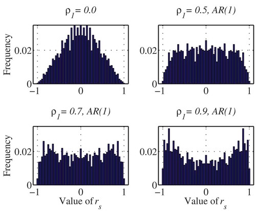
Figure 1 shows the exact distribution of Spearman’s rho for n = 7 for different values of the first-order autocorrelation coefficient for the case of AR(1) as an example. The effect of persistence on the distribution is clear, where the distribution becomes flatter and the tails become heavier as persistence increases, to the extent of producing a bimodal distribution in the case of AR(1) data for this small sample size. The non-smooth nature of the distribution of rho compared to that of Kendall’s tau (cf. Hamed 2008) may help explain the slow convergence of the distribution to the normal, which becomes even slower with the added effect of persistence on the tails of the distribution.

Figure 1. The exact distribution of Spearman’s rho for AR(1) data with different values of ρ₁ and sample size n = 7.

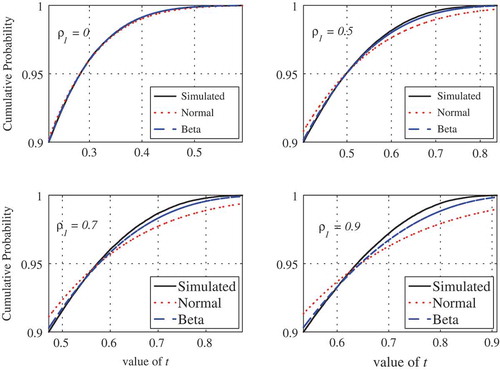
The exact distribution for small samples (n < 10) is mainly intended for theoretical purposes and comparison with earlier work, since relatively longer time series are needed in practice in order to reliably assess trends, especially in the presence of persistence. For practical problems it would be more efficient to approximate the full distribution using a suitable probability distribution. After investigating several candidate probability distributions, the beta distribution was found to be suitable as an approximation to the distribution of rho for moderate values of the sample size n (say n < 50), similar to the case of Kendall’s tau (Hamed 2009). The single parameter of the symmetric beta distribution can be obtained using the variance calculated from equation (15). The reader is referred to Hamed (2009) for details. Figure 2 shows a comparison between the simulated distribution for a sample of size n = 10, along with the beta and normal approximations for different values of the first-order autocorrelation coefficient. The superiority of the beta approximation for persistent data is evident from Fig. 2. As the sample size increases, however, the differences between the two approximations become smaller, but not as fast as in the case of non-persistent data. Figure 3 shows the case for a sample size n = 35, where the beta distribution performs much better at higher values of the first-order autocorrelation coefficient. In fact, the beta distribution remains superior to the normal distribution for large sample sizes (n > 50), but the differences become too small to justify using the beta approximation. An interesting feature, however, which can be clearly observed in both Figs 2 and 3, is that both the beta and normal approximations coincide with the actual distribution near the probability of 0.95. In fact, this was also found to be true for the case of Kendall’s tau. This suggests that the normal distribution would be a reasonable approximation, even for small sample sizes, for the particular significance level of 5% (one-sided).

Figure 2. Comparison of simulated and approximate distributions of Spearman’s rho for a sample of size n = 10.

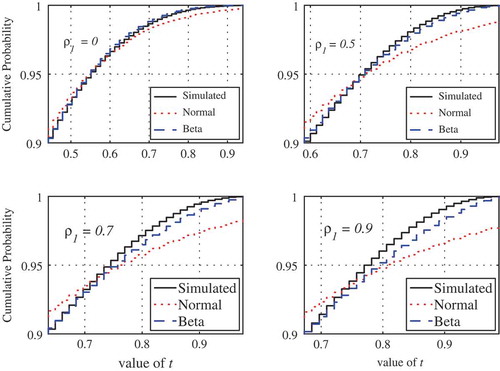
Figure 3. Comparison of simulated and approximate distributions of Spearman’s rho for a sample of size n = 35.

4 Case study

The aim of this case study is to illustrate the effect of persistence on trend test results using Spearman’s rho, and to show the equivalence of the results to those obtained by using Kendall’s tau. The trend tests based on Spearman’s rho and Kendall’s tau are applied to a group of world river flow time series that have been studied earlier by Hamed (2008) using the Mann-Kendall trend test. The data were kindly supplied by the Global Runoff Data Centre in Koblenz, Germany (http://grdc.bafg.de). Hamed (2008) has shown that a large number of stations exhibited a significant scaling behaviour. For the purposes of this study, and in order to show the equivalence of the two studied test statistics for persistent data, only stations with scaling coefficients that are significant at the 5% level (20 stations) are considered. Details of these 20 stations are given in Table 5.

Table 5. Details of river flow stations used in the case study.

No.	Station ID	River	Station	Country	Time period	n
1	1134100	Niger	Koulikoro	ML	1907–2001	95
2	2964122	Chao Phraya	Khai Chira Prawat	TH	1956–2000	45
3	4113300	Red River	Grand Forks	US	1904–2005	102
4	4115310	Kettle	Near Ferry	US	1928–2005	78
5	4119080	St. Croix	St. Croix Falls	US	1910–2005	96
6	4121160	White	Near Oacoma	US	1928–2005	78
7	4122100	Elkhorn	Waterloo	US	1928–2004	77
8	4123111	Little Wabash	Carmi	US	1939–2005	67
9	4123278	New	Near Galax	US	1929–2005	77
10	4147540	Saddle	Lodi	US	1923–2005	83
11	4152550	Green	Green River	US	1906–2005	100
12	4207180	Nechako	Isle Pierre	CA	1950–2003	54
13	4214210	Beaver	Cold Lake Reserve	CA	1955–2005	51
14	5204105	Murrumbidgee	Mittagang Crossing	AU	1927–2000	74
15	5302250	Thomson	Cooper Creek	AU	1956–2001	46
16	6335350	Lahn	Leun (Neu)	DE	1935–2004	70
17	6335500	Main	Wuerzburg	DE	1823–2001	179
18	6731280	Austena	Austena	NO	1925–2000	76
19	6731300	Etna	Etna	NO	1920–2000	81
20	6855500	Karjaanjoki	Lohjanjarvi-Peltokoski	FI	1938–2004	67

An important problem in testing the significance of trends in persistent data is the estimation of persistence parameter(s). Since one cannot tell a priori if an observed trend is a real trend or not (this is why a trend test is being performed in the first place), one has to account for the interaction between trend and persistence. On one hand, if one ignores a real trend, the estimated persistence parameter(s) will be inflated, resulting in the inflation of the variance of the trend test statistic, thus reducing the significance of the real trend. On the other hand, if one removes an apparent stochastic trend, the persistence parameter(s) will be underestimated, resulting in deflation of the variance of the trend test statistic, thus increasing the significance of the apparent (false) trend. This is in addition to the fact that persistence parameters are usually downward biased even in the trend-free case (cf. Hamed 2007). Hamed (2008) suggests a two-step approach to overcome this difficulty. First, apparent trends are removed from the data using a suitable non-parametric trend estimate, such as Sen’s estimator (Sen 1968), which can be calculated as

(20)

The second step involves compensating for the underestimation of the persistence parameters by applying a bias correction factor obtained by simulation using purely persistent data (i.e. without trends). Hamed (2008) uses a bias correction factor for the variance of Kendall’s tau. Following the same procedure, a bias correction factor B for the variance of Spearman’s rho has been estimated using 10 000 samples of FGN data with different values of the scaling coefficient and different sample sizes as

(21)

where H_Det is the sample scaling coefficient estimated from the data after removing an apparent trend, n is the sample size, and

To correct for the bias due to the underestimation of the scaling parameter H and due to the removal of apparent trends, the variance calculated from equation (16) using the autocorrelation function of the FGN model in equation (18) with a scaling parameter H_Det is multiplied by the coefficient B from equation (21).

The results of applying both Spearman’s rho and Kendall’s tau trend tests on the selected flow station data are given in Table 6. The first column in Table 6 gives the station ID number. The second and third columns give the estimated scaling coefficients H for the original data, and H_Det for the detrended data, respectively. The fourth column gives the ratio between the sample estimates of Spearman’s rho, r_s, and Kendall’s tau, t. The fifth to seventh columns compare the variance inflation factor, the p value of the original test (without taking the effect of persistence into account), and the corrected p value of the test (after accounting for the effect of persistence) for Spearman’s rho and Kendall’s tau (in parentheses), respectively.

Table 6. Comparison between trend test results using Spearman’s rho and Kendall’s tau (in parentheses) for selected world river flow stations. Bold face indicates significant trend at the 5% level.

Station ID	H	HDet	rs/t	Variance inflation	Original p value	Corrected p value (considering persistence)
(a) Increasing trend
4113300	0.86	0.78	1.54	9.36 (9.77)	9.2 × 10^–6 (1.1 × 10^–5)	8.1 × 10^–2 (8.8 × 10^–2)
4115310	0.65	0.58	1.40	2.61 (2.63)	3.6 × 10^–2 (2.7 × 10^–2)	1.3 × 10^–1 (1.2 × 10^–1)
4119080	0.87	0.76	1.50	7.81 (8.14)	1.2 × 10^–6 (1.5 × 10^–6)	4.6 × 10^–2 (5.1 × 10^–2)
4121160	0.60	0.58	1.50	2.59 (2.61)	5.7 × 10^–2 (5.3 × 10^–2)	1.6 × 10^–1 (1.6 × 10^–1)
4122100	0.79	0.73	1.49	6.49 (6.64)	3.4 × 10^–6 (2.8 × 10^–6)	3.9 × 10^–2 (3.9 × 10^–2)
4123111	0.67	0.62	1.47	3.41 (3.39)	1.3 × 10^–2 (1.3 × 10^–2)	1.1 × 10^–1 (1.1 × 10^–1)
4123278	0.70	0.66	1.33	4.17 (4.23)	1.7 × 10^–2 (1.2 × 10^–2)	1.5 × 10^–1 (1.4 × 10^–1)
4147540	0.64	0.60	1.53	2.82 (2.87)	2.0 × 10^–2 (2.2 × 10^–2)	1.1 × 10^–1 (1.2 × 10^–1)
6335350	0.67	0.60	1.56	3.08 (3.07)	1.1 × 10^–2 (1.3 × 10^–2)	9.5 × 10^–2 (1.0 × 10^–1)
6335500	0.72	0.68	1.44	4.87 (5.20)	4.0 × 10^–2 (3.7 × 10^–2)	2.1 × 10^–1 (2.2 × 10^–1)
6855500	0.65	0.58	1.33	2.77 (2.74)	4.3 × 10^–3 (2.4 × 10^–3)	5.7 × 10^–2 (4.4 × 10^–2)
(b) Decreasing trend
1134100	0.89	0.83	1.54	13.3 (13.7)	6.1 × 10^–5 (7.8 × 10^–5)	1.5 × 10^–1 (1.5 × 10^–1)
2964122	0.67	0.64	1.23	4.27 (4.15)	3.9 × 10^–2 (1.7 × 10^–2)	2.0 × 10^–1 (1.5 × 10^–1)
4152550	0.75	0.67	1.42	4.45 (4.64)	3.6 × 10^–4 (2.0 × 10^–4)	5.4 × 10^–2 (5.0 × 10^–2)
4207180	0.74	0.73	1.44	6.55 (6.54)	2.3 × 10^3 (2.1 × 10^–3)	1.3 × 10^–1 (1.3 × 10^–1)
4214210	0.70	0.64	1.36	4.19 (4.09)	7.8 × 10^–4 (2.9 × 10^–4)	6.1 × 10^–2 (4.4 × 10^–2)
5204105	0.75	0.68	1.54	4.93 (5.01)	1.6 × 10^–7 (3.6 × 10^–7)	1.1 × 10^–2 (1.3 × 10^–2)
5302250	0.79	0.65	1.45	4.60 (4.48)	1.2 × 10^–4 (8.6 × 10^–5)	4.4 × 10^–2 (4.1 × 10^–2)
6731280	0.63	0.59	1.45	2.78 (2.79)	8.4 × 10^–2 (8.9 × 10^–2)	2.0 × 10^–1 (2.1 × 10^–1)
6731300	0.64	0.60	1.57	2.93 (2.97)	2.7 × 10^–2 (3.0 × 10^–2)	1.3 × 10^–1 (1.4 × 10^–1)

The results in Table 6 clearly show the extent of the adverse effect of persistence on trend test results using Spearman’s rho as well as Kendall’s tau. While the original tests indicate that 18 out of 20 stations had significant trends at the 5% level (10 increasing and eight decreasing), this number drops to four stations (two increasing and two decreasing) in the case of Spearman’s rho, and five stations (two increasing and three decreasing) in the case of Kendall’s tau, a reduction of more than 70%. The ratios between the sample values of rho and tau in the fourth column vary slightly around their expected value of 3/2 = 1.5, and the variance inflation factors in the fifth column are very close as expected. The p values of the original test in the sixth column are very close, resulting in the same conclusions from either test. The corrected p values in the seventh column are also very close, although slight differences, such as in the case of stations 4119080, 6855500 and 4214210, would suggest different conclusions at the 5% level. However, such slight differences will always occur due to the sampling variation of rho and tau, and the p values for any given station may lie very close to, but on different sides of the critical limit for any given significance level. It can thus be concluded that, similar to the case of independent data covered previously in the literature, trend tests based on Spearman’s rho and Kendall’s tau still give effectively identical results for persistent data, for both the original and the corrected tests.

5 Conclusions

The distribution of Spearman’s rho for persistent data has been considered, and an expression for the variance of the test statistic for persistent data has been developed, together with a method for evaluating the full distribution of rho for small samples. An approximation of the distribution for moderate sample sizes has also been suggested, while the normal distribution approximation can be used for large samples. The effect of persistence on the inflation of the variance of Spearman’s rho has been shown to be comparable to that for Kendall’s tau. A case study of trends in a number of world river flow stations reveals that the p-values resulting from applying the two tests are almost identical. These results confirm the equivalence of the two statistics for testing trends in persistent data. However, the fast convergence of Kendall’s tau to the normal distribution makes it preferable to Spearman’s rho in small samples.

Disclosure statement

No potential conflict of interest was reported by the author.

Acknowledgements

The author would like to thank the Associate Editor, Salvatore Grimaldi, and two anonymous reviewers for their helpful comments. The data used in the case study were kindly provided by the Global Runoff Data Centre (GRDC) in Koblenz, Germany.

References

- Fredricks, G.A. and Nelsen, R.B., 2007. On the relationship between Spearman’s rho and Kendall’s tau for pairs of continuous random variables. Journal of Statistical Planning and Inference, 137, 2143–2150. doi:10.1016/j.jspi.2006.06.045
- Grimaldi, S. and Serinaldi, F., 2006. Design hyetograph analysis with 3-copula function. Hydrological Sciences Journal, 51 (2), 223–238. doi:10.1623/hysj.51.2.223
- Hamed, K.H., 2007. Improved finite-sample Hurst exponent estimates using rescaled range analysis. Water Resources Research, 43, W04413. doi:10.1029/2006WR005111
- Hamed, K.H., 2008. Trend detection in hydrologic data: the Mann–Kendall trend test under the scaling hypothesis. Journal of Hydrology, 349 (3–4), 350–363. doi:10.1016/j.jhydrol.2007.11.009
- Hamed, K.H., 2009. Exact distribution of the Mann-Kendall trend test statistic for persistent data. Journal of Hydrology, 365, 86–94. doi:10.1016/j.jhydrol.2008.11.024
- Hamed, K.H., 2011. The distribution of Kendall’s tau for testing the significance of cross-correlation in persistent data. Hydrological Sciences Journal, 56 (5), 841–853. doi:10.1080/02626667.2011.586948
- Kendall, M.G. and Gibbons, J.D., 1990. Rank correlation methods. 5th edition. London: Griffin.
- Kendall, M.G. and Stuart, A., 1976. The advanced theory of statistics. Vol. I: distribution Theory. London: Griffin.
- Moran, P.A.P., 1948. Rank correlation and product-moment correlation. Biometrika, 35, 203–206. doi:10.1093/biomet/35.1-2.203
- Sen, P.K., 1968. Estimates of the regression coefficient based on Kendall’s tau. Journal American Statistics Association, 63, 1379–1389. doi:10.1080/01621459.1968.10480934
- Yue, S., Pilon, P., and Cavadias, G., 2002. Power of the Mann-Kendall and Spearman’s rho tests for detecting monotonic trends in hydrological series. Journal of Hydrology, 259, 254–271. doi:10.1016/S0022-1694(01)00594-7