Robust informational entropy-based descriptors of flow in catchment hydrology

Abstract

This paper explores the use of entropy-based measures in catchment hydrology, and provides an importance-weighted numerical descriptor of the flow–duration curve. Although entropy theory is being applied in a wide spectrum of areas (including environmental and water resources), artefacts arising from the discrete, under-sampled and uncertain nature of hydrological data are rarely acknowledged, and have not been adequately explored. Here, we examine challenges to extracting hydrologically meaningful entropy measures from a flow signal; the effect of binning resolution on calculation of entropy is investigated, along with artefacts caused by (1) emphasis of information theoretic measures towards flow ranges having more data (statistically dominant information), and (2) effects of discharge measurement truncation errors. We introduce an importance-weighted entropy-based measure to counter the tendency of common binning approaches to over-emphasise information contained in the low flows which dominate the record. The measure uses a novel binning method, and overcomes artefacts due to data resolution and under-sampling. Our analysis reveals a fundamental problem with the extraction of information at high flows, due to the lack of statistically significant samples in this range. By separating the flow–duration curve into segments, our approach constrains the computed entropy to better respect distributional properties over the data range. When used as an objective function for model calibration, this approach constrains high flow predictions, as well as the commonly used Nash-Sutcliffe efficiency, but provides much better predictions of low flow behaviour.

Editor Z.W. Kundzewicz

Associate editor Not assigned

Keywords:

• entropy
• binning
• hydrological signal
• flow–duration curve
• truncation error

1 Introduction

Hydrological fluxes (e.g. precipitation, streamflow) and water resources systems are dominated by spatio-temporal complexities that limit our understanding of the underlying physical processes. In practice, hydrology is frequently faced with less than adequate data (e.g. sparse and noisy observations) to describe the behaviour of such systems. Despite these difficulties, a major aim of the hydrological community is to describe causal relationships between hydrological quantities (Beven 2001, Koutsoyiannis 2010, Pechlivanidis et al. 2011). While time series partial correlation analysis can extract properties of coupling between different variables, it is unable to capture the strength of nonlinear relationships between different variables (Knuth 2005, Markowetz and Spang 2007).

Information theory provides a powerful approach to closing fundamental gaps in our ability to relate multiple interconnected data streams to process understanding. Probability-based information measures make no assumptions about the nature of underlying system dynamics or the relationships among system variables (e.g. they capture any-order correlations among the time series). Consequently, they provide a promising avenue to identify where information is present and/or conflicting. Ultimately, information theoretic computations rely upon quantities such as entropy and, therefore, the past decade has seen entropy concepts applied to a range of problems in hydrology and water resources (see reviews by Singh 1997, 2000). These applications encompass derivation of frequency distributions and estimation of their parameters (Singh and Guo 1995), monitoring and evaluation of networks and flow forecasting (Krstanovic and Singh 1993, Yang and Burn 1994, Ozkul et al. 2000, Mogheir and Singh 2002), investigation of the spatio-temporal characteristics of precipitation fields (Molini et al. 2006, Brunsell 2010), hydrological processes (Koutsoyiannis 2005a, 2005b; Ruddell and Kumar 2009), and runoff series (Hauhs and Lange 2008).

Information theory can also provide insights into hydrological theory. Singh (2010a) defined parameters of infiltration equations (e.g. Horton, Kostiakov, Philip, Green-Ampt, Overton and Holtan) in terms of information measures, i.e. Shannon entropy and the principle of maximum entropy (POME). Singh (2010b) applied the Tsallis entropy and POME to describe water flow in unsaturated soils; similar studies by Pachepsky et al. (2006) and Al-Hamdan and Cruise (2010) used the Shannon entropy instead.

An interesting use of entropy-based measures is as objective functions in the calibration of hydrological models. In the first such published application, Amorocho and Espildora (1973) explored the uses and limitations of entropy and mutual information for assessing hydrological model performance. Chapman (1986) recommended the ratio of mutual information to marginal entropy as a model performance measure. Recently, Pechlivanidis et al. (2010a) noted Shannon entropy’s strong relationship to the flow–duration curve (FDC) and showed that, although insensitive to timing errors, entropy-based measures provide useful diagnostics when used in combination with other objective functions. Pokhrel and Gupta (2011) showed that an entropy-based measure is more sensitive to subtle differences in streamflow time series (caused by spatial variability in precipitation and parameter fields) than conventional criteria (i.e. mean square error).

As indicated above, hydrologists have been estimating entropy from the probability density (pdf) of data for years. However, uncertainties associated with the computation of entropy using discrete data have not always been acknowledged (Weijs et al. 2013a, 2013b). Entropy measures depend on the accurate estimation of probability densities from the data. A key choice is the binning method used to discretise the data probability distribution, a necessary step in calculating the Shannon entropy of a continuous variable (Cover and Thomas 1991, Scott 1992). Binning methods include fixed width (Molini et al. 2006) and fixed mass (Ruddell and Kumar 2009); studies show that calculated values of entropy and mutual information can depend on the binning resolution (Amorocho and Espildora 1973, Chapman 1986, Blower and Kelsall 2002) and sample size (Molini et al. 2006). Other studies in the fields of coding, machine learning, signal processing and chemistry have investigated artefacts arising from the interpolation methods used to calculate mutual information (Pluim et al. 1999, Gómez-Verdejo et al. 2009). Knuth et al. (2006) developed tools to describe the degree of uncertainty in entropy estimates due to the number of bins. Despite these advances, the estimation of entropy remains an open problem (Nilsson and Kleijn 2007, Srivastava and Gupta 2008, Larson 2010). Calculation of entropy from flow data introduces a second aspect of discretisation, i.e. discrete sampling of flow and truncation of the flow measurement. To our knowledge, no study has investigated artefacts arising in the use of entropy to extract information from discrete flow signals or, more generally, from any noise and truncation-error contaminated environmental time series.

Further, despite the wide application of entropy-based measures in hydrology, there has been no formal association of the probabilistic Shannon entropy measure with the flow–duration curve. The FDC is simply the cumulative density function of streamflow and is widely considered to be a hydrologically informative “signature” of catchment behaviour (Farmer et al. 2003, Son and Sivapalan 2007, Wagener et al. 2007). FDCs have been used in a range of hydrological applications including model calibration (Yu and Yang 2000, Westerberg et al. 2011), water management (Cole et al. 2003), regionalisation (Niadas 2005), and classification of catchment morphology and behaviours (Castellarin et al. 2001, Hauhs and Lange 2008). Analytical FDC forms are rarely used (but see Castellarin et al. 2004, Serinaldi 2011), consequently, entropy measures of flow are generally calculated using discrete models.

This paper investigates the use of entropy-based measures for extracting static (non-dynamic) information from streamflow signals via the FDC. We investigate the effects of binning resolution on calculation of entropy, along with artefacts such as (1) statistical insufficiency of samples, (2) tendency of the metrics to emphasise flow ranges containing more data, and (3) flow measurement truncation error and uncertainty. Section 2 introduces the study area and data used. Entropy-based properties are introduced in Section 3, where we also highlight barriers to robust implementation in the hydrological context. Section 4 presents a practical example consisting of statistical analysis based on observed and modelled flow data, followed by a discussion in Section 5. Finally, Section 6 states the conclusions.

2 Study site and data description

We illustrate our discussion using data from the Mahurangi River (Fig. 1(a)) in northern New Zealand, which drains 46.6 km² of steep hills and gently rolling lowlands. The Mahurangi River Variability Experiment, MARVEX (Woods et al. 2001), investigated the space–time variability of the catchment water balance from 1997 to 2001. A network of 28 flowgauges and 13 raingauges collected records at 15-minute intervals (Woods 2004). The catchment experiences a warm humid climate (frosts are rare and snow and ice are unknown), with mean annual rainfall and evaporation of 1600 and 1310 mm, respectively. Catchment elevation ranges from sea level to 300 m. The soils are mainly clay loams, no more than a metre deep, and much of the lowland area is used for grazing. Plantation forestry occupies most of the hills in the south, and a mixture of native forest, scrub and grazing occurs on the hills in the north. For further details see Woods (2004).

Figure 1. (a) The Mahurangi River catchment, and (b) the catchment’s flow–duration curve.

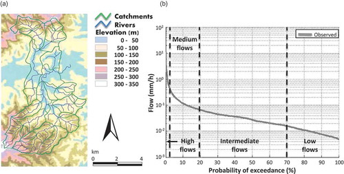
Historical rainfall, streamflow and potential evapotranspiration data at hourly time steps were provided by the National Institute of Water and Atmospheric Research, New Zealand, for the period 1998–2001. The arithmetic average of 13 raingauge records was used as the estimate of mean areal precipitation and considered to be distributed uniformly over the catchment. Only the flow data from the catchment outlet gauge were considered in the present study; the corresponding FDC is presented in Fig. 1(b).

3 Methods

3.1 Information theory metrics

Entropy (in Greek εντροπία, etymologised from τροπή, i.e. change, turn, drift) is variously described; examples include a measure “of the uncertainty associated with a random variable” or “of the lack of information about the system” (Koutsoyiannis 2005a). Shannon (1948) defined entropy as a quantitative measure of the information content of a signal, i.e.

(1)

where p(x_i) is the probability of outcome x_i of the discrete, non-negative random variable X such that , M is the number of possible outcomes and E[ ] denotes expected value. Here we use a base 2 logarithm so entropy is the average number of binary digits (bits) needed to optimally encode X following p(x_i). Shannon entropy takes values between 0 (complete information) and log₂(M) (no information), but is commonly normalised by log₂(M) to lie in (0,1). Low values of entropy indicate a high degree of departure from a uniform distribution and low uncertainty.

A continuous analog to Shannon entropy exists for continuous X with probability density f(x) satisfying . This continuous Shannon entropy, otherwise known as differential entropy (Jaynes 2003), is defined as

(2)

This definition is not fully consistent with its discrete counterpart. The entropy of a discrete variable can be infinite when the number of bins is infinite, whereas the entropy of a continuous variable is finite. Koutsoyiannis (2005a) shows that (1) the entropy of a discrete variable is always positive whereas that of a continuous variable may be positive, zero or negative, and (2) in the discrete case, the value of entropy does not depend on the variable X that is used to quantify the description of the phenomenon; however, it depends on the variable X in the continuous case.

As hydrological data are generally discretised (e.g. stage measurements to the nearest mm) and their frequency distribution cannot be accurately derived from a limited number of observations, hydrological uses of Shannon entropy have naturally treated the underlying distribution as discrete, applying equation (1). As we show later, discretisation requires several subjective choices; see also Weijs et al. (2013b) for a detailed discussion of these subjective choices. While it would be possible to specify an analytical form for the underlying flow probability distribution and apply equation (2), such estimation presents a different and arguably more complex set of issues; not least uncertainties in estimating the probability distribution. Further, discrete and continuous entropies are not directly comparable, as noted above. This difference also precludes the use of synthetic data conditioned on a theoretical probability distribution for use in evaluating entropy metrics based on equation (2). Metrics must instead be tested in their ability to reproduce a pdf of discrete observed data using equation (1), as we do in this paper. We therefore follow the convention of previous applications to hydrology, and focus on identifying and overcoming artefacts caused by the discrete calculation.

The objective of this paper is to contribute to the development of robust, hydrologically relevant measures of Shannon entropy suitable for application to discrete hydrological signals. Given that most entropy measures are derived from Shannon entropy, strategies for making this computation more robust are likely to be at least in part applicable to the rest. As such, our comments and findings also apply to related measures such as relative entropy, mutual information (Mogheir and Singh 2002, Mishra et al. 2009), transfer entropy (Schreiber 2000, Ruddell and Kumar 2009), etc.

3.2 Methods for transforming discrete data to entropy metrics

We used two methods to calculate entropy metrics from discrete flow data: (1) Define bin boundaries and count the number of data points in each bin. (2) Estimate the continuous pdf underlying the flow data, then define bin centroids and evaluate the pdf at these centroids, and use each centroid as an outcome x_i in equation (1).

For method (1), different approaches can be used to discretise the dataset into probability bins. With too few/many partitions, “edge effects” become severe and entropy estimates are positively biased (Ruddell and Kumar 2009). The methods include binning with fixed mass, fixed width or hybrid fixed width–mass interval partitions (Ruddell and Kumar 2009, Pechlivanidis et al. 2012). Fixed width interval partitions are usually applied since the approach is simple and computationally efficient (Ruddell and Kumar 2009). In this study, we compare the relative merits of applying fixed width intervals (e.g. linear and logarithmic), fixed mass interval (e.g. equal probability), hybrid fixed width–mass interval (e.g. combination of linear and equal probability) partitions, and kernel estimation to the Mahurangi dataset described in Section 2.

For method (2), we use the semi-continuous method of nonparametric kernel estimation, which does not require specification of a bin resolution (and hence is not affected by artefacts arising from this). Instead, it introduces a narrowly peaked probability density function at each data point and sums each of these functions to obtain the entire density. Admittedly artefacts still can arise due to its sensitivity to the smoothing function defined by a “bandwidth” parameter; however, these have been more widely studied in the literature and we used an accepted and objective optimisation approach (proposed by Botev et al. 2010) to minimise such artefacts (see Appendix A).

3.3 Effects of binning resolution

In this section, we use the Mahurangi dataset to illustrate the advantages and disadvantages of different binning methods.

Linear binning uses a constant bin width over the full range of the pdf, while logarithmic binning utilises logarithmic spacing. Equally probable partitioning requires the same number of data points to be present within each bin¹ ; to achieve this despite limited precision data points, we added small amplitude normal noise before binning (Knuth et al. 2005).

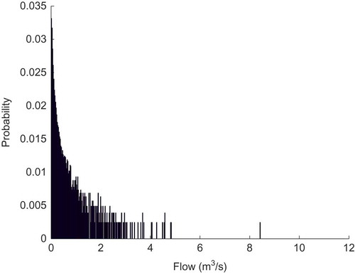
The probability distribution being discretised by these different approaches is shown in Fig. 2. Results show that flows below 0.05 mm/h dominate the streamflow time series. Consequently, bins discretised following the equal probability interval approach will have fine resolution at low flow values but coarse resolution at high values (e.g. >1 mm/h). Similarly, bins derived from the logarithmic binning approach still have fine resolution at low flows and coarse resolution at high values, though not as severely as the equal probability approach. Due to their similar emphasis on low flow ranges, the results provided by logarithmic and equal probability binning approaches are similar, and therefore only the equal probability approach is presented in this paper. When the linear approach is used, the bins are uniformly distributed over the flow range and the probability distribution of low flows is poorly estimated. However, the linear method better represents the probability distribution associated with medium to high flow values than the other two approaches.

Figure 2. Probability distribution of the flow values for the Mahurangi catchment.

To overcome weaknesses in the conventional binning methods, and to achieve a better representation of the full range of flow measurements, we introduce a hybrid fixed width–mass binning method. Our approach helps to extract the static distributional information over the sparsely sampled medium and high flow characteristics as well as the densely sampled low flow characteristics. Typical hydrological applications may be interested in adequate representation of low (e.g. >70%), intermediate (e.g. 20–70%), medium (e.g. 2–20%) and high (e.g. <2%) flows, although certain hydrological objectives (e.g. water resources, flood forecasting) may emphasise a more limited range. For demonstration, we use these ranges applied to the Mahurangi catchment; values are 0.2, 0.7 and 8.6 m³/s (0.014, 0.053 and 0.664 mm/h) respectively. These values of the flow bin edges may change in accordance with study objectives and catchment characteristics.

The number of bins selected a priori was defined using an optimal binning identification tool by Knuth (2005). The tool uses Bayesian probability theory to evaluate the marginal posterior probability of the number of bins in a piecewise-constant density function model of the distribution from which the data were sampled. This posterior probability originates as a product of the likelihood of the density parameters given the data and the prior probability of those same parameter values. The result that maximises the logarithm of the probability is selected. Figure 3 presents the un-normalised log posterior probability for the Mahurangi streamflow data for number of linear bins varying between 1 and 800. The log posterior probability is also estimated for data within each segment of the flow–duration curve (high, medium, intermediate and low).

Figure 3. The log posterior probability for different numbers of bins and for different segments of the Mahurangi’s FDC.

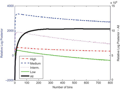
Based on this analysis, 500 bins are identified to describe the underlying probability density for the full range of the Mahurangi streamflow data (“All” line in Fig. 3). Similarly, 26, 20, 20 and 23 bins are identified to maximise the marginal posterior probability at the high, medium, intermediate and low segments of the FDC, respectively (see Fig. 3)—these numbers of bins are used in this analysis. We introduced a second constraint that bin width should not be less than the precision of the data. This constraint did not affect the binning in any flow category.

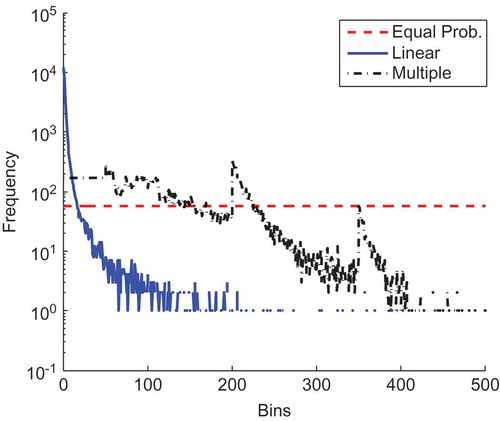
Figure 4 shows the frequency for each bin using the equally probable, linear and multiple binning approaches. Equal probability binning places 58 values in each bin, while linear binning places almost 10⁴ values (1/3 of the time series) into the first bin and consequently the frequencies above the 20th linear bin are significantly reduced (less than 10 values per bin). The multiple binning approach enables better control of the frequency distribution; the flow frequency is fixed for low flow values since bins are equally probable; however, frequency varies for the other three flow ranges. The same pattern is observed in these groups, with the frequency being reduced at high flows due to the lack of high records within the available time series.

Figure 4. Flow frequency for each bin using different partition methods.

3.4 Comparing entropy differences between flow signals—a metric respecting both mass conservation and shape

Up to this point, we have considered the calculation of entropy of a stand-alone signal. We now consider the additional challenges faced when attempting to compare entropy between two different flow signals. For example, we may wish to compare entropy values computed from observed and simulated flows, or flow entropy differences between multiple catchments or time periods. Shannon entropy quantifies the distribution of values within a dataset, with no sensitivity to differences in timing. In addition, this probability-based measure is not usually discretised to depend on the range of the data, so mass balance errors can be introduced. For example, consider three streamflow hydrographs (Q_t, Q_t/2, and Q_t+DT), where Q_t/2 is the streamflow data of Q_t divided by 2 at each time step, while Q_t+DT is the Q_t data lagged by DT hours. Entropy considers the probability that a value (or range of values) occurs within the data series, and does not take into account their location within the time series. Therefore, the three hydrographs have identical Shannon entropy.

As mass conservation is important in many hydrological applications, for instance when comparing observed and simulated streamflow sequences, time series analysis based on the Shannon entropy may need to introduce methods that account for mass balance. A performance measure with sensitivity to mass balance can be obtained by using a single set of bins, with their range being set to encompass both modelled and measured data values. To distinguish between the binning methods, we refer to the scaled Shannon Entropy, H^S, as the one computed using identical bins for both time series (simulated and observed data; this attempts to conserve mass and shape), and unscaled Shannon Entropy, H^U, as the one computed using different bin ranges for each time series based on their individual specific maximum range (this respects shape conservation, and hence information, irrespective of mass/scaling).

Based on this, we propose an entropy-based metric suitable for hydrological applications that recognises the trade-off between Scaled and Unscaled Shannon Entropy differences, SUSE. The value of SUSE is defined as

(4)

We estimate this metric using each of the four binning resolutions: linear, equally probable, multiple bins, and the continuous kernel density function. Note that the range of SUSE lies between 0 (perfect agreement) and 1. A value of SUSE larger than zero indicates that the entropy of the simulated time series differs from the entropy of the observed time series.

3.5 A hydrologically relevant entropy difference metric

To better characterise the FDC, we propose a new metric, the Conditioned Entropy Difference (CED), which we define as the maximum entropy difference present in the different FDC segments:

(5)

where m is the number of the FDC segments, and sg is the probability of exceedence for each segment of the FDC. Our aim in defining the CED metric is to draw information from all hydrologically relevant segments of the FDC. For the Mahurangi data, we selected four segments of the FDC (0–2, 2–20, 20–70, and 70–100%) as previously described for the multiple binning approach (Section 3.3).

4 Practical example

In this section, we illustrate and test the usefulness of the different entropy metrics we have defined, by applying them as performance measures for calibration of a hydrological model. We tested both the SUSE metric with different binning approaches, and the CED metric, and compared the results to the Nash-Sutcliffe efficiency as a benchmark. Our analysis includes checking for sensitivity to the subjective choices inherent in the CED.

4.1 Model identification

To illustrate our discussion, we use the six-parameter Probability Distributed Moisture (PDM) model (Moore 1985, 2007, Pechlivanidis et al. 2010b) to simulate hourly streamflow for the Mahurangi catchment. Total streamflow is delayed by 2 hours to adjust the time to peak response (the routing delay model parameter was manually adjusted). This removes sensitivity to timing errors and focuses the analysis on the shape of the FDC. The first year (1998) is used as a model warm-up period, the next two years (1999–2000) for model calibration, and the final year (2001) for independent performance evaluation. A Monte Carlo uniform random search is used to explore the feasible parameter space and to investigate parameter identifiability and inter-dependence (150 000 samples). We note this is not a comprehensive sample of the entire parameter space; the number of samples is a balance between statistical accuracy and computational constraints. However, given the parsimonity of the model (only six parameters), it is thought to be adequate for demonstration purposes. More sophisticated sampling methods such as Markov Chain Monte Carlo might better explore the near-optimal spaces, but would limit our ability to explore parameter interdependence.

To calibrate the model, we use four versions of the SUSE entropy-based measure, using various binning methods: linear (Linear), equally probable (Equal Prob.), multiple bins (Multiple), and the continuous kernel density function (Kernel). As a benchmark, we compare the results to use of the NSE performance measure (NSE = 1 − var(residuals)/var(flows)) (Nash and Sutcliffe 1970). The latter has been widely applied in hydrology as a benchmark measure of fit; it can also be interpreted as a classic skill score (Murphy 1988), where skill is interpreted as the comparative ability with regards to a baseline model (here taken to be the “mean of the observations”—i.e. values of NSE less than 0 indicate that the mean of the observed time series provides, on average, a better predictor than the model). The range of NSE lies between 1 (perfect fit) and −∞.

To identify behavioural model parameter sets we use a threshold value for the performance measures: NSE > 0.7 and SUSE < 0.13. Although these threshold values are subjective, NSE values greater than 0.7 are generally considered acceptable in many hydrological applications (see Freer et al. 2004). Threshold values for SUSE are chosen so that the number of behavioural SUSE parameter sets is similar to the number of behavioural NSE sets (901 in here). We also explore the sensitivity of the results to different SUSE threshold values (see Section 4.3). However, our objective is not to conduct parameter sensitivity analysis based on the NSE thresholds, but to compare results based on the entropy metrics against a benchmark hydrological measure (i.e. NSE). When conditioning the four segments of the FDC, we require that behavioural model parameter sets simultaneously satisfy the threshold condition at all segments. More generally, a weighting scheme could be introduced by setting higher thresholds to measures of the FDC segments that are less important for an application’s objectives (e.g. a flood prediction study can allow a higher threshold for the entropy measure at low flows and lower threshold at high flows).

4.2 Biases in identification resulting from use of entropy difference metrics

The first step was to establish the potential of each objective function to enable a successful calibration of the model. This was achieved using the NSE as a benchmark. Table 1 shows calibration and evaluation results using the five objective functions. The first column indicates the criterion used for model calibration. The next sets of columns indicate the calibration and evaluation period values achieved for each of the five performance measures by the calibrated parameter set so obtained. For instance, the first set of columns shows that good NSE performance is achieved on both the calibration and evaluation periods when using the multiple bins (row 6) and kernel density (row 7) methods (NSE > 0.7). However, use of linear binning (row 4) provides poor performance (on average associated NSE values were 0.54) and equally probable binning (row 5) provides even worse performance (on average associated NSE values were 0.25). This result highlights the lack of consistency in model performance between entropy values based on common binning approaches, and hence their limitation as stand-alone measures in hydrological modelling.

Table 1. Model performance for calibration and evaluation period using the five objective functions (NSE, and SUSE using the four binning methods). Each column presents the objective function value using the “optimum” model parameter set based on the objective function of the first column. NSE is maximised while SUSE is minimised. The diagonal bold values present the individual model performances.

	NSE		Linear		Equal Prob.		Multiple		Kernel
	Cal.	Eval.	Cal.	Eval.	Cal.	Eval.	Cal.	Eval.	Cal.	Eval.
NSE	0.86	0.80	0.06	0.05	0.10	0.11	0.03	0.06	0.05	0.06
Linear	0.53	0.55	0.00	0.11	0.19	0.23	0.31	0.31	0.01	0.11
Equal Prob.	0.26	0.24	0.30	0.40	0.01	0.05	0.05	0.04	0.20	0.26
Multiple	0.79	0.72	0.03	0.07	0.04	0.09	0.00	0.04	0.01	0.02
Kernel	0.81	0.75	0.02	0.06	0.06	0.10	0.01	0.04	0.00	0.00

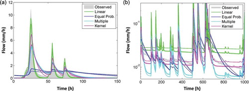
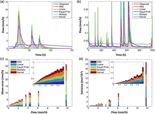
Figure 5(a) and 5(b) illustrates the model fit achieved using the optimum parameter set identified based on the five objective functions during a high and a low flow period, respectively. Figure 5(c) and 5(d) shows the mean absolute error and variance for the dataset using the behavioural parameter sets respectively (NSE > 0.7 and SUSE < 0.13 for each binning approach). Simulated runoff based on Equal Prob. binning is biased towards information in low flow data, but both high flow (Fig. 5(a)) and low flow recessions (Fig. 5(b)) are badly represented. Linear binning provides the best fit to the highest flow event (10.7 mm/h), but fitting during low flows is poor. The multiple binning approach and kernel density estimation both provide a reasonable fit to both low and high flows (although both approaches underestimate the highest flow peak).

Figure 5. Simulated streamflow using the optimum model parameter set for the five measures during (a) high flow period and (b) low flow period. (c) and (d) The distribution of mean absolute error and variance using the behavioural model parameter sets (NSE > 0.7 and SUSE < 0.13) for the five measures respectively.

We next examine performance of the entropy-based metrics in regards to reproduction of signature measures (Table 2), to examine biases towards specific properties of the FDC. Formulae for the signature measures are presented in Appendix B. Significant bias is observed at the low segment when Linear entropy is used, highlighting the importance of the binning resolution and the number of bins at this range. Table 2 (columns 3–7) shows that NSE performs better than the entropy measures at high flow ranges; however, the four entropy measures achieve smaller bias in all other aspects of the FDC. Kernel entropy achieves the second best performance during high flow periods (mean absolute bias 15%), indicating its suitability for flood prediction applications, although relatively poor performance is achieved at the low and intermediate segments of the FDC. Equal Prob. is unable to represent high flows well (on average 38.9% bias), but achieves the smallest bias at the other aspects of the FDC.

Table 2. Signature metrics for each FDC segment using the five objective functions (NSE and SUSE using the four binning methods). Results are based on the behavioural model parameter sets. The bold values present the metrics with the lowest bias for each FDC segment.

		NSE	Linear	Equal Prob.	Multiple	Kernel
		> 0.7	< 0.13	< 0.13	< 0.13	< 0.13
High volume bias (%)	Mean	12.8	18.7	38.9	24.8	15.0
	Variance	60.6	153.8	151.8	141.6	149.9
Intermediate slope bias (%)	Mean	45.2	51.0	16.4	28.2	52.3
	Variance	697.2	1226.7	146.8	330.9	1127.2
Low volume bias (%)	Mean	33.3	34.1	25.7	21.8	33.0
	Variance	234.6	485.3	377.3	223.5	513.6
Midflow bias (%)	Mean	12.2	16.1	6.3	9.7	13.9
	Variance	110.7	172.9	14.0	50.9	95.7

4.3 Results using the conditioned entropy difference metric (CED)

To overcome biases towards specific ranges of flow values caused by a single entropy measure (as shown in Table 2), we now evaluate the CED approach which estimates entropy differences for each segment of the FDC; equally probable binning is used for the low flow segment of the FDC, whereas linear binning is used to capture information from the intermediate, medium and high flow segments (see Sec. 3.5).

4.3.1 Choice of behavioural threshold

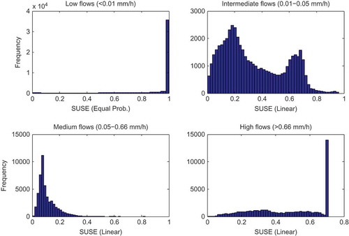
It is not practical to use the same behavioural threshold for each of the FDC segments, as it is much harder to match observed and simulated low and high flow entropies than moderate flow entropies. This is illustrated in Fig. 6, which shows histograms of normalised scores for each segment, from our initial 150 000 Monte Carlo samples. For example, in the low flow segment, only around 1500 model parameter sets (out of 150 000) are able to achieve entropy differences lower than 0.1, indicating that the model structure may not be capable of representing low flows well. For the results presented here, we chose threshold values of 0.15, 0.1, 0.1 and 0.1 for the low, intermediate, medium and high FDC segments, respectively (thresholds that also allow a reasonably adequate number of behavioural sets). These values could be varied according to the modelling objectives. One important aspect of future work will be to develop objective strategies for selection of these thresholds.

Figure 6. Frequency distribution of entropy difference metric for low, intermediate, medium and high flow values. The x-axis shows the value of the entropy difference metric and the y-axis shows the frequency of the metric values in the stated segment of the FDC.

4.3.2 Benchmark comparison of CED with NSE using single threshold

To investigate the potential of the CED metric, streamflow is simulated based on the behavioural model parameter sets selected using this measure and compared to those selected using NSE. A threshold (0.13) was used to identify the CED behavioural sets (although this value is subjective, the sensitivity of the results to different threshold values is further explored), while for NSE we use the 905 parameter sets resulting in NSE > 0.7. Results are illustrated in Fig. 7 for high and low flow periods. Use of CED results in underestimation of peaks. The trade-off between entropy for low and high flows and the fixed threshold (i.e. 0.13) for each entropy metric could have an effect on the identification of the conditioned parameter sets. It is also important to note that out of the 3 years of hourly data (a year is used for warm up), there are only 390 flow values within the high flow range (<2%). As a result, there may not be a significantly large sample of high flows to accurately represent the probability distribution. Figure 7(b) shows that use of the NSE ensemble results in very wide ranges at low flows, whereas the CED ensemble is narrower for baseflow. Overall, Fig. 7 highlights the trade-off between the entropy metrics at low and high flows; we cannot avoid trade-offs due to data and structural errors.

Figure 7. Simulated streamflow during (a) high flow and (b) low flow periods using the behavioural parameter sets based on the NSE and CED.

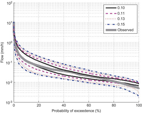
We next investigate the effect of the choice of the CED threshold on the simulated runoff and hence the FDC. Figure 8 shows the envelope of the FDCs using the CED metric for different threshold values (0.10, 0.11, 0.13 and 0.15; the numbers of behavioural parameter sets are 10, 33, 117 and 277, respectively). As expected, the envelope narrows when the threshold value decreases. Note that the differences in the FDC envelopes between a threshold of 0.15 and 0.13 are not visually significant except at low flows; however, there is a marked change when moving from a threshold of 0.13 to 0.10. It should also be noted that the low flow tail is not adequately captured as the threshold is decreased, probably due to the model structure deficiency; multiple tanks might be required to capture the recessions in the Mahurangi (McMillan et al. 2011).

Figure 8. FDC using the CED-based model parameter sets for various threshold values.

4.3.3 Benchmark comparison of CED with NSE using multiple thresholds

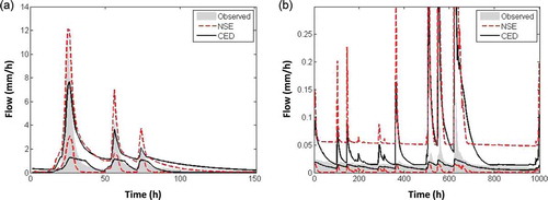
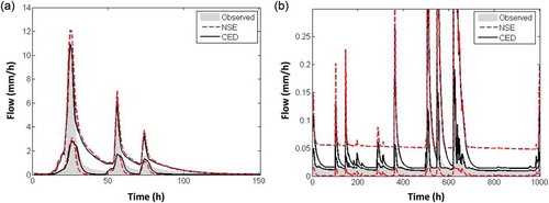
To address the importance of threshold values, we show how the choice of multiple threshold values can produce a significant improvement in the CED entropy as an objective function. Figure 9 presents the simulated runoff for high and low flow periods using 0.15, 0.1, 0.1 and 0.1 as thresholds for the four segments of the FDC. The range of simulated runoff during the high flow period is similar using the NSE and the CED parameter sets. There is only a slight overestimation of the peaks when the NSE is used. However, the NSE-conditioned ensemble is significantly over-dispersed for low flow periods. The potential of the CED measure is illustrated in Fig. 9(b), where the envelope of simulated runoff remains very close to the baseflow. Figure 9 demonstrates that use of CED as an objective function can constrain high flow predictions equally well as the NSE, while simultaneously providing well-constrained low flow predictions that the NSE is unable to achieve.

Figure 9. Simulated streamflow during (a) high flow and (b) low flow periods using the behavioural parameter sets based on the NSE and CED.

4.3.4 Effect of multiple thresholds on fitted flow pdf

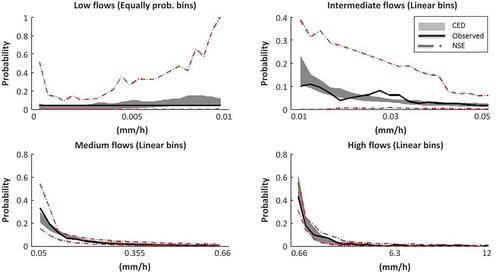
We finally investigate the ability of the multiple thresholds CED metric to reproduce the probability distribution at each segment of the FDC (Fig. 10). The results show significant improvement in identification of conditioned model parameter sets relative to the NSE over all segments, particularly marked in the case of the low and intermediate flow periods. However, some trade-offs in performance between segments still exist (presumably in part due to deficiencies in the selected model structure or driving data). It is important to recognise this and select threshold values appropriate to the modelling question; for example, a high threshold on the low segment will give less emphasis to low flows, potentially deteriorating performance here while forcing the optimisation procedure to emphasise fit to distributional properties of the medium and high flows.

Figure 10. Probability distribution at the different segments of the FDC using the behavioural parameter sets based on the NSE and CED.

5 Discussion

5.1 Information entropy: one- and two-dimensional case (objective function)

The SUSE metric proposed in this paper overcomes many of the artefacts influencing estimation of entropy for streamflow variables, and the derived CED metric importance weights this information over multiple flow ranges to better respect the distributional properties over ranges of particular interest. The measure is designed to enhance fits to less-sampled but still statistically significant ranges. The very highest flow values remain under-sampled and hence are not statistically robust. Although entropy measures assign higher information per observation to the least frequent values, SUSE and CED demand a respectable sample per range so still assign little overall significance to these hardly sampled extremes. This is demonstrated by the tendency of CED to provide a good fit to most of the data range except the highest, most infrequent flow values. A fundamental issue remains: hydrological datasets can be limited in their lack of statistically significant samples over key ranges of interest, and are by definition limited at their extremes. Taking this further, where flow ranges do not have a statistically significant sample, entropy estimates, and any objective function measures derived from them, are unreliable; we cannot use data to “learn” about reality for ranges without (statistically significant) data. One way to partially overcome this would be to use interpolation to increase the number of data samples at this under-sampled range, but this is arguably dangerous due to the lack of statistical significance of existing samples (adding “information” not present in the dataset). From a philosophical point of view, it is worth noting that in many applications measures such as NSE are forced to match data of low statistical significance (e.g. high flow values). Due to their emphasis on reducing absolute differences, they can end up highly biased towards naively respecting those statistically insignificant, highly uncertain ranges.

Another issue to be noted is that entropy-based measures (and hence the CED metric) rely on probability distribution functions. However, pdfs of streamflow measurements are subject to errors caused by uncertainty in the stage and velocity measurements, and rating curves used to transform continuously measured stage values into discharge values. Additional challenges to those we have discussed in this paper can be expected to arise when estimating entropy for particularly erroneous discharge measurements (our techniques account for noise in streamflow measurements, but not for error bias). A possible way to assess the impact of streamflow data uncertainty on the calculation of entropy measures would be to use an “envelope rating curve” (upper and lower acceptable limits on discharge measurements) (Liu et al. 2009, McMillan et al. 2010).

Entropy is strongly sensitive to the static (non-dynamic) information contained in the pdf of the flow data and hence of the flow–duration curve, used as a signature of catchment behaviour. It is insensitive to timing errors, which limits its potential as a stand-alone performance measure; however, it is increasingly acceptable in hydrology that multi-performance measures are needed for calibration to target different aspects of system behaviour (Gupta et al. 2008). For instance, the combination of CED with performance measures that target information in the signal that the CED alone cannot characterise (i.e. temporal auto-correlation and dynamic properties of the flow signal) could achieve better performance over the full range of flow values and drive model calibration in a diagnostic manner. Entropy-based measures provide a promising avenue to decouple timing errors from other errors, and hence may assist us to diagnose model/data/hypotheses inconsistencies. In principle, this approach is fundamental for a robust framework for model evaluation, considering the amount of information in the data, and maximum extraction of information from the data. At this point, we also use a comment from Weijs et al. (2010, p. 2556):

This is especially important in calibration, where a model has to learn from observations. When calibration objectives are used that are not information-measures, the model either learns from information that is not there or uses only part of the information in the observations, or both. Because the amount of available information is related to optimal model complexity, hydrological models trained for user specific utilities are more prone to overfitting, which might lead to worse results in an independent validation test.

5.2 Development of case oriented information-based metrics—future work

The SUSE (and consequently CED) measures are based on Shannon entropy, which is quantified for a single time series. However, our proposed approach can be expanded to other entropy-based measures, i.e. relative entropy. Measures based on relative entropy concepts could potentially provide a more compelling descriptor of the difference between observed and simulated flow results than the CED metric developed here. Empirically the CED has provided an excellent indicator of fit between observed and simulated flow “shape” and mass (relative to more established measures) in the explorations we have carried out to date. However, theoretical arguments tell us it will fail under some conditions; different distributional shapes can produce the same entropy. Perhaps most importantly, although a perfect fit would always be correctly identified, it is possible (although extremely unlikely given other constraints) for a dissimilar fit to also be incorrectly identified as a perfect fit. This would not be possible using a relative entropy measure appropriately adjusted to reduce artefacts, as we have done for the Shannon entropy.

An initial analysis into the potential of relative entropy was carried out, conditioning models using a scaled/unscaled relative entropy measure (SUSRE) rather than Shannon entropy. Overall the fit to the FDC characteristics was degraded; there were slight improvements in the low flows but the performance in the high flows was degraded using SUSRE (see Appendix C). However, further work analysing the sensitivity of relative entropy to the various methodological choices and parameterisations causing artefacts, and adjusting those choices accordingly, might well improve current results. We would expect a measure based on relative entropy to be insightful and potentially to have higher predictive power, and less risk of misidentification, for models with high degrees of freedom. We suspect that model parsimony, along with additional constraints provided by physical thresholds/driving data and the structural properties of catchments (effectively low pass filters), provide a degree of protection from the theoretical potential of SUSE or other entropy difference-based measures to misidentify similarities or dissimilarities between observed and simulated flow responses.

We also recommend that future work should use mutual information to analyse the information contained in the modelled and observed data or quantify the overlap of the information content of multiple (sub)systems, or identify the changes in the properties of a system. Transfer entropy should be used to determine the directionality, relative strength, time lag and scale of information flow that couples multiple (sub)systems or quantify the information flow between the input and output of a system. Future reports of our ongoing research will introduce the CED in a multi-objective framework to provide a useful diagnostic to decouple timing and other errors.

6 Summary and conclusions

We have explored the potential use of entropy-based measures in catchment hydrology with particular attention to extracting the static, distributional information contained within a streamflow signal. We demonstrate a number of calculation artefacts that can occur when applying common entropy techniques to discrete uncertain flow data, arising from the choice of bin divisions, sampling bias (which for example can arise from the tendency of flow data to have over-sampled low flows and under-sampled high flows), truncation error and data uncertainty. We found that use of common linear or fixed mass binning approaches is inadequate for describing the structure in the flow signal.

As a step towards overcoming such problems, we introduce an entropy-based metric, which we call the Conditioned Entropy Difference (CED), that separates the FDC into multiple segments and applies binning techniques appropriate to those segments (equally probable intervals in the low segment and linear intervals in the intermediate, medium and high flow segments), thereby constraining the entropy estimate to respect distributional properties of the data. This metric overcomes artefacts due to data resolution (truncation error) and can incorporate a tolerance to uncertainty by adjusting the a priori specified number of bins. Entropy is estimated for each individual segment, and normalised according to the number of data points so the metric is comparable between segments and between datasets. This importance-weighted, conditioned entropy measure can extract the still statistically significant but not statistically dominant information; CED overcomes the tendency of entropy to emphasise information within the low (most sampled) flows by estimating the entropy over multiple segments of the FDC. By conditioning entropy to respect multiple segments of the FDC, we can re-weight entropy to respect those parts of the flow distribution of most interest to the application.

A case study using hourly observed and simulated data from the Mahurangi catchment in New Zealand showed that use of CED as an objective function for model calibration can constrain high flow predictions as well as the traditional NSE metric, while simultaneously providing well-constrained low flow predictions that the NSE is unable to achieve. Although use of CED as a stand-alone objective metric could be dangerous as it is theoretically possible for dissimilar signals to be misidentified as similar, it may have high potential as a complementary measure. Work to extend the importance weighting and artefact reduction for extended information theoretic measures (e.g. relative and mutual entropy) is also likely to be beneficial.

Matlab codes developed to estimate entropy at segments of the FDC and using the binning approaches presented in this paper are available from the first author.

Disclosure statement

No potential conflict of interest was reported by the author.

Acknowledgments

The authors thank Dr Vazken Andréassian and Professor Demetris Koutsoyiannis for their fruitful discussions during this investigation and Dr Steven Weijs for his constructive review suggestions and recommendations which significantly improved this paper. Thanks also to New Zealand’s National Institute of Water and Atmospheric Research (NIWA) for providing the dataset used in this study.

Notes

¹ Equally probable partitions are equivalent to the maximisation of entropy. This is related to the concept of maximum entropy (see details in Kapur 1989) using only the constraint .

Appendix A

The nonparametric kernel density estimation method directly determines the shape of the nonparametric density function from the data, and requires no assumptions about the distribution of the population of interest or estimation of parameters (e.g. mean, variance and skewness) (Wand and Jones 1995). For a given kernel function K() and a given sample x₁, x₂,…, x_n, the kernel estimator of a probability density function at each fixed point x is given by

(A1)

where is the kernel estimator of unknown real density function f(x), K() is a kernel function that must integrate to unity, is the sample standard deviation, h is a parameter called bandwidth (or smoothing factor), and n is the number of sample data.

Several kernel functions (e.g. Gumbel and Epanechnikov) have been used in hydrology (Guo et al. 1996, Wang and Ding 2007). The choice of kernel function is not critical and the shape of kernel does not affect extrapolation accuracy (Adamowski 2000), therefore we chose for the current study a Gaussian kernel function. However, the choice and calculation by the data of the bandwidth coefficient, h, is critical. Too high h results in an oversmoothed density estimator , some of whose characters (modes and asymmetries) are smoothed out, and the estimator has a high bias and low variance (Wang and Ding 2007). On the other hand, a small h results in an approximate density estimator with small bias and large variance. The mean integrated square error MISE () = E∫[ − f(x)]²dx of the estimator is often adopted as a criterion to evaluate the kernel estimator precision. The bandwidth for the observed streamflow of the Mahurangi catchment is 0.00038.

In this study, we used the Kernel Density Estimator Matlab code by Botev et al. (2010), which estimates the kernel density based on linear diffusion processes. The estimator built on an approach for adaptive smoothing by incorporating information from a pilot density estimate. The authors note that the bandwidth selection method is free from the arbitrary normal reference rules used by existing methods. The code estimates the probability density of the data at 2¹⁴ points within the data range; hence the probability density is assumed semi-continuous.

Appendix B

This appendix presents the equations of the FDC signature measures referenced in this paper. The absolute percentage bias in FDC high-segment volume is

(B1)

where h = 1, 2, …, H are the flow indices for flows with exceedence probabilities lower than 0.02.

The measure for medium flow values is the absolute percentage bias in FDC intermediate-segment slope, described as

(B2)

where m1 and m2 are the lowest and highest flow exceedence probabilities (0.2 and 0.7, respectively) within the intermediate segment of the FDC.

The measure for FDC low-segment volume is

(B3)

where l = 1, 2, …, L is the index of the flow value located within the low flow segment (0.7–1.0 flow exceedence probabilities) of the flow duration curve, L being the index of the minimum flow.

The midflow behaviour measure was calculated using the median value of the observed (Qobs_med) and simulated (Qsim_med) flows as an index and is estimated as

(B4)

Appendix C

In this appendix, we present an initial analysis into the potential of relative entropy, conditioning models using a scaled/unscaled relative entropy measure (SUSRE) rather than Shannon entropy (SUSE). Other methodological choices and parameterisations (binning methods, thresholds, etc.) remained as per the SUSE /CED analyses. Figure C1 illustrates the model fit achieved using the optimum parameter set identified based on SUSRE (dashed lines) during the high and low flow periods. Results for SUSE are also reproduced from Fig. 5 and presented with thin solid lines to allow comparison with SUSRE. As concluded for SUSE, fitting of flow characteristics (recession, peaks and baseflow) using SUSRE is sensitive to the binning approach; linear binning is sensitive to high flows, while kernel seems to provide an “average” fit to both low and high flows. Overall, peaks during high flows are more underestimated using SUSRE than SUSE (particularly when multiple binning is considered); however it seems that SUSRE slightly improves the fitting during low flows in comparison to SUSE.

Figure C1. Simulated streamflow using the optimum model parameter set for the relative entropy measures (SUSRE; dashed lines) and SUSE measures (thin solid lines) during (a) high flow and (b) low flow periods.

References

- Adamowski, K., 2000. Regional analysis of annual maximum and partial duration flood data by nonparametric and L-moment methods. Journal of Hydrology, 229, 219–231. doi:10.1016/S0022-1694(00)00156-6
- Al-Hamdan, O.Z. and Cruise, J.F., 2010. Soil moisture profile development from surface observations by principle of maximum entropy. Journal of Hydrologic Engineering, 15 (5), 327–337. doi:10.1061/(ASCE)HE.1943-5584.0000196
- Amorocho, J. and Espildora, B., 1973. Entropy in the assessment of uncertainty in hydrologic systems and models. Water Resources Research, 9 (6), 1511–1522. doi:10.1029/WR009i006p01511
- Beven, K., 2001. Rainfall–runoff modelling. The primer. Chichester, UK: John Wiley and Sons, 1–360.
- Blower, G. and Kelsall, J., 2002. Nonlinear Kernel density estimation for binned data: Convergence in entropy. Bernoulli, 8 (4), 423–449.
- Botev, Z.I., Grotowski, J.F., and Kroese, D.P., 2010. Kernel density estimation via diffusion. The Annals of Statistics, 38 (5), 2916–2957. doi:10.1214/10-AOS799
- Brunsell, N.A., 2010. A multiscale information theory approach to assess spatial–temporal variability of daily precipitation. Journal of Hydrology, 385 (1–4), 165–172. doi:10.1016/j.jhydrol.2010.02.016
- Castellarin, A., Burn, D.H., and Brath, A., 2001. Assessing the effectiveness of hydrological similarity measures for flood frequency analysis. Journal of Hydrology, 241 (3–4), 270–285. doi:10.1016/S0022-1694(00)00383-8
- Castellarin, A., et al., 2004. Regional flow duration curves: reliability for ungauged basins. Advances in Water Resources, 27 (10), 953–965. doi:10.1016/j.advwatres.2004.08.005
- Chapman, T.G., 1986. Entropy as a measure of hydrologic data uncertainty and model performance. Journal of Hydrology, 85, 111–126. doi:10.1016/0022-1694(86)90079-X
- Cole, R.A.J., Johnston, H.T., and Robinson, D.J., 2003. The use of flow duration curves as a data quality tool. Hydrological Sciences Journal, 48 (6), 939–951. doi:10.1623/hysj.48.6.939.51419
- Cover, T. and Thomas, J., 1991. Elements of information theory. New York: John Wiley & Sons.
- Farmer, D., Sivapalan, M., and Jothityangkoon, C., 2003. Climate, soil, and vegetation controls upon the variability of water balance in temperate and semiarid landscapes: downward approach to water balance analysis. Water Resources Research, 39 (2), 1035. doi:10.1029/2001WR000328
- Freer, J.E., et al., 2004. Constraining dynamic TOPMODEL responses for imprecise water table information using fuzzy rule based performance measures. Journal of Hydrology, 291 (3–4), 254–277. doi:10.1016/j.jhydrol.2003.12.037
- Gómez-Verdejo, V., Verleysen, M., and Fleury, J., 2009. Information-theoretic feature selection for functional data classification. Neurocomputing, 72, 3580–3589. doi:10.1016/j.neucom.2008.12.035
- Guo, S.L., Kachroo, R.K., and Mngodo, R.J., 1996. Nonparametric kernel estimation of low flow quantiles. Journal of Hydrology, 185, 335–348. doi:10.1016/0022-1694(95)02956-7
- Gupta, H., Wagener, T., and Liu, Y., 2008. Reconciling theory with observations: elements of a diagnostic approach to model evaluation. Hydrological Processes, 22 (18), 3802–3813. doi:10.1002/hyp.6989
- Hauhs, M. and Lange, H., 2008. Classification of runoff in headwater catchments: A physical problem? Geography Compass, 2 (1), 235–254. doi:10.1111/j.1749-8198.2007.00075.x
- Jaynes, E.T., 2003. Probability theory. Cambridge, U.K: Cambridge University Press, 727.
- Kapur, J.N., 1989. Maximum entropy models in science and engineering. New York: Wiley.
- Knuth, K.H., 2005. Lattice duality: the origin of probability and entropy. Neurocomputing, 67, 245–274. doi:10.1016/j.neucom.2004.11.039
- Knuth, K.H., Castle, J.P., and Wheeler, K.R. 2006. Identifying excessively rounded or truncated data. (Invited Submission), Proceedings of the 17th meeting of The International Association for Statistical Computing-European Regional Section: Computational Statistics (COMPSTAT 2006), August, Rome, Italy.
- Knuth, K.H., et al., 2005. Revealing relationships among relevant climate variables with information theory. In Proceedings of the Earth-Sun System Technology Conference (ESTC 2005), July, Adelphi, MD.
- Koutsoyiannis, D., 2005a. Uncertainty, entropy, scaling and hydrological statistics. 1. Marginal distributional properties of hydrological processes and state scaling. Hydrological Sciences Journal, 50 (3), 381–404. doi:10.1623/hysj.50.3.381.65031
- Koutsoyiannis, D., 2005b. Uncertainty, entropy, scaling and hydrological stochastics. 2. Time dependence of hydrological processes and time scaling. Hydrological Sciences Journal, 50 (3), 405–426. doi:10.1623/hysj.50.3.405.65028
- Koutsoyiannis, D., 2010. HESS Opinions “A random walk on water”. Hydrology and Earth System Sciences, 14 (3), 585–601. doi:10.5194/hess-14-585-2010
- Krstanovic, P.F. and Singh, V.P., 1993. A real-time flood forecasting model based on maximum-entropy spectral analysis: II. Application. Water Resources Management, 7, 131–151. doi:10.1007/BF00872478
- Larson, J.W., 2010. Can we define climate using information theory? IOP Conference Series: Earth and Environmental Sciences, 11 (1), 012028. doi:10.1088/1755-1315/11/1/012028.
- Liu, Y., et al., 2009. Towards a limits of acceptability approach to the calibration of hydrological models: Extending observation error. Journal of Hydrology, 367 (1–2), 93–103. doi:10.1016/j.jhydrol.2009.01.016
- Markowetz, F. and Spang, R., 2007. Inferring cellular networks - a review. BMC Bioinformatics, 8 (Suppl 6), S5. doi:10.1186/1471-2105-8-S6-S5
- McMillan, H., et al., 2011. Hydrological field data from a modeller’s perspective: Part 1. Diagnostic tests for model structure. Hydrological Processes, 25 (4), 511–522. doi:10.1002/hyp.7841
- McMillan, H., et al., 2010. Impacts of uncertain river flow data on rainfall–runoff model calibration and discharge predictions. Hydrological Processes, 24 (10), 1270–1284.
- Mishra, A.K., Özger, M., and Singh, V.P., 2009. An Entropy-based Investigation into the Variability of Precipitation. Journal of Hydrology, 370, 139–154. doi:10.1016/j.jhydrol.2009.03.006
- Mogheir, Y. and Singh, V.P., 2002. Application of Information Theory to Groundwater Quality Monitoring Networks. Water Resources Management, 16 (1), 37–49. doi:10.1023/A:1015511811686
- Molini, A., La Barbera, P., and Lanza, L.G., 2006. Correlation patterns and information flows in rainfall fields. Journal of Hydrology, 322 (1–4), 89–104. doi:10.1016/j.jhydrol.2005.02.041
- Moore, R.J., 1985. The probability-distributed principle and runoff production at point and basin scales. Hydrological Sciences Journal, 30 (2), 273–297. doi:10.1080/02626668509490989
- Moore, R.J., 2007. The PDM rainfall–runoff model. Hydrology and Earth System Sciences, 11 (1), 483–499. doi:10.5194/hess-11-483-2007
- Murphy, A., 1988. Skill scores based on the mean square error and their relationships to the correlation coefficient. Monthly Weather Review, 116, 2417–2424. doi:10.1175/1520-0493(1988)116<2417:SSBOTM>2.0.CO;2
- Nash, J.E. and Sutcliffe, J.V., 1970. River flow forecasting through conceptual models part I — A discussion of principles. Journal of Hydrology, 10, 282–290. doi:10.1016/0022-1694(70)90255-6
- Niadas, I.A., 2005. Regional flow duration curve estimation in small ungauged catchments using instantaneous flow measurements and a censored data approach. Journal of Hydrology, 314 (1–4), 48–66. doi:10.1016/j.jhydrol.2005.03.009
- Nilsson, M. and Kleijn, W.B., 2007. On the estimation of differential entropy from data located on embedded manifolds. IEEE Transactions on Information Theory, 53 (7), 2330–2341. doi:10.1109/TIT.2007.899533
- Ozkul, S., Harmancioglu, N.B., and Singh, V.P., 2000. Entropy-based assessment of water quality monitoring networks in space/time dimensions. Journal of Hydrologic Engineering, 5 (1), 90–100. doi:10.1061/(ASCE)1084-0699(2000)5:1(90)
- Pachepsky, Y., et al., 2006. Information content and complexity of simulated soil water fluxes. Geoderma, 134 (3–4), 253–266. doi:10.1016/j.geoderma.2006.03.003
- Pechlivanidis, I.G., et al., 2011. Catchment scale hydrological modelling: A review of model types, calibration approaches and uncertainty analysis methods in the context of recent developments in technology and applications. Global NEST Journal, 13 (3), 193–214.
- Pechlivanidis, I.G., Jackson, B., and McMillan, H. 2010a. The use of entropy as a model diagnostic in rainfall–runoff modelling. In iEMSs 2010: International Congress on Environmental Modelling and Software, 5–8 July, Ottawa, Canada.
- Pechlivanidis, I.G., et al., 2012. Using an informational entropy-based metric as a diagnostic of flow duration to drive model parameter identification. Global NEST Journal, 14 (3), 325–334.
- Pechlivanidis, I.G., McIntyre, N., and Wheater, H.S., 2010b. Calibration of the semi-distributed PDM rainfall-runoff model in the Upper Lee catchment, UK. Journal of Hydrology, 386 (1–4), 198–209. doi:10.1016/j.jhydrol.2010.03.022
- Pluim, J.P.W., Maintz, J.B.A., and Viergever, M.A., 1999. Mutual information matching and interpolation artefacts. SPIE Medical Imaging 1999. Image Processing, 3661, 1–10.
- Pokhrel, P. and Gupta, H.V., 2011. On the ability to infer spatial catchment variability using streamflow hydrographs. Water Resources Research, 47, W08534. doi:10.1029/2010WR009873
- Ruddell, B.L. and Kumar, P., 2009. Ecohydrologic process networks: 1. Identification. Water Resources Research, 45, W03419. doi:10.1029/2008WR007279
- Schreiber, T., 2000. Measuring information transfer. Physical Review Letters, 85 (2), 461–464. doi:10.1103/PhysRevLett.85.461
- Scott, D.W., 1992. Multivariate density estimation: Theory, practice, and visualization. New York: Willey.
- Serinaldi, F., 2011. Analytical confidence intervals for index flow flow duration curves. Water Resources Research, 47, W02542. doi:10.1029/2010WR009408.
- Shannon, C.E., 1948. A mathematical theory of communication. Bell System Technical Journal, 27, 379–423. (Part I) and 623-656 (Part II), doi:10.1002/j.1538-7305.1948.tb01338.x.
- Singh, V.P., 1997. The use of entropy in hydrology and water resources. Hydrological Processes, 11 (6), 587–626. doi:10.1002/(SICI)1099-1085(199705)11:6<587::AID-HYP479>3.0.CO;2-P
- Singh, V.P., 2000. The entropy theory as a tool for modelling and decision-making in environmental and water resources. Water SA, 26 (1), 1–11.
- Singh, V.P., 2010a. Entropy theory for derivation of infiltration equations. Water Resources Research, 46, W03527. doi:10.1029/2009WR008193
- Singh, V.P., 2010b. Entropy theory for movement of moisture in soils. Water Resources Research, 46, W03516. doi:10.1029/2009WR008288
- Singh, V.P. and Guo, H., 1995. Parameter estimation for 3-parameter generalized Pareto distribution by the principle of maximum entropy (POME). Hydrological Sciences Journal, 40, 165–181. doi:10.1080/02626669509491402
- Son, K. and Sivapalan, M., 2007. Improving model structure and reducing parameter uncertainty in conceptual water balance models through the use of auxiliary data. Water Resources Research, 43 (1), W01415. doi:10.1029/2006WR005032
- Srivastava, S. and Gupta, M.R. 2008. Bayesian estimation of the entropy of the multivariate Gaussian. In IEEE International Symposium on Information Theory, 6–11 July, Toronto, ON, 103–107.
- Wagener, T., et al., 2007. Catchment classification and hydrologic similarity. Geography Compass, 1 (4), 901–931. doi:10.1111/j.1749-8198.2007.00039.x
- Wand, M.P. and Jones, M.C., 1995. Kernel smoothing. MR1319818. Chapman and Hall: London, 212.
- Wang, W. and Ding, J., 2007. A multivariate non-parametric model for synthetic generation of daily streamflow. Hydrological Processes, 21, 1764–1771. doi:10.1002/hyp.6340
- Weijs, S.V., Schoups, G., and Van De Giesen, N., 2010. Why hydrological predictions should be evaluated using information theory. Hydrology and Earth System Sciences, 14 (12), 2545–2558. doi:10.5194/hess-14-2545-2010
- Weijs, S.V., Van De Giesen, N., and Parlange, M.B., 2013a. Data compression to define information content of hydrological time series. Hydrology and Earth System Sciences, 17, 3171–3187. doi:10.5194/hess-17-3171-2013
- Weijs, S.V., Van De Giesen, N., and Parlange, M.B., 2013b. HydroZIP: How hydrological knowledge can be used to improve compression of hydrological data. Entropy, 15, 1289–1310. doi:10.3390/e15041289
- Westerberg, I. K., et al., 2011. Calibration of hydrological models using flow duration curves. Hydrology and Earth System Sciences, 15, 2205–2227, doi:10.5194/hess-15-2205-2011.
- Woods, R.A., 2004. The impact of spatial scale on spatial variability in hydrologic response: Experiments and ideas. Scales in Hydrology and Water Management, 287, 1–15.
- Woods, R.A., et al., 2001. Experimental design and initial results from the Mahurangi River Variability Experiment: MARVEX. In: V. Lakshmi, J.D. Albertson, and J. Schaake, eds. Observations and modelling of land surface hydrological processes. Water Resources Monographs. Washington, DC: American Geophysical Union, 201–213.
- Yang, Y. and Burn, D.H., 1994. An entropy approach to data collection network design. Journal of Hydrology, 157 (1–4), 307–324. doi:10.1016/0022-1694(94)90111-2
- Yu, P.-S. and Yang, T.-C., 2000. Using synthetic flow duration curves for rainfall–runoff model calibration at ungauged sites. Hydrological Processes, 14 (1), 117–133. doi:10.1002/(SICI)1099-1085(200001)14:1<117::AID-HYP914>3.0.CO;2-Q